Generic Correlation Model for Wireless Sensor ...

Generic Correlation Model for Wireless Sensor Network Applications

RESEARCH ARTICLE April 2012 Research Work at IITK

ISSN 2043-6394

IET WSS

Rajeev K. Shakya, Yatindra N. Singh , Nishchal K. Verma

Generic Correlation Model for Wireless Sensor Network Applications Rajeev K. Shakya∗ , Yatindra N. Singh ∗ , Nishchal K. Verma

∗

Research Work at IITK Research Report no. – — version final† — initial version April 2012 — revised version May 2013 — 21 pages

Abstract: In Wireless Sensor Networks (WSNs) having a high density of sensor nodes, transmitted measurements are spatially correlated, often redundantly whenever an event of interest is detected. In this work, we propose a correlation model to enable energy-efficient methodologies that exploit the spatial correlation at the Network and MAC layers. At the Network layer, we first demonstrate how, through proper tuning of both the sensing range and the correlation threshold, WSNs can be partitioned into disjoint correlated clusters without degrading the information reliability, thus enabling significant energy saving. On the other hand, as another contribution, we investigate the impacts of correlation between nodes on achieved distortion in the event estimation at the sink. The interactions among various parameters such as distortion constraints, spatial node density, node selection, sensing range and their impacts on the reconstruction performance are quantitatively studied. We demonstrate that the same level of distortion constraint can be achieved by selecting fewer nodes. The nodes can be still fewer if they are less spatially correlated. However the MAC protocols which show distributive effect of this selection needs more study. Key-words: wireless sensor networks, virtual coordinate system, application constraints, MAC, routing

∗

Department of Electrical Engg., Indian Institute of Technology, Kanpur, Kanpur (U.P.), 208016, India This paper is a postprint of a paper submitted to and accepted for publication in “IET Wireless Sensor Networks" and is subject to Institution of Engineering and Technology Copyright. The copy of record is available at IET Digital Library †

This paper is a postprint of a paper submitted to and accepted for publication in “IET Wireless Sensor Networks" and is subject to Institution of Engineering and Technology Copyright.

The copy of record is available at IET Digital Library.

Correlation Model

2

Generic Correlation Model for Wireless Sensor Network Applications Biography : Rajeev K. Shakya received B.E. degree in Electronics & Instrumentation Engineering in 2003 and M.E. degree in Electrical Engineering in May 2007, both from Shri G.S.Institute of Technology and Science, Indore (MP), INDIA. Currently, he is a PhD candidate in Electrical Department, Indian Institute of Technology, Kanpur (UP), INDIA. His major research interests include energy-efficient node clustering, scheduling, and correlation-based communication protocols for wireless sensor networks. He is a student member of the IEEE. Yatindra Nath Singh received B.Tech. in Electrical Engineering with honors from Regional Engineering College, Hamirpur, Himachal Pradesh in July 1991, M.Tech. in Optoelectronics & Optical Communications from India Institute of Technology, Delhi in December 1992 and Ph.D. from Department of Electrical Engineering, Indian Institute of Technology, Delhi in 1997. He was with the Department of Electronics and Computer Engineering, IIT Roorkee, India as faculty from Feb’97 to July’97. He is currently working as faculty in department of electrical engineering, Indian Institute of Technology, Kanpur. He is a fellow of Institution of Electronics and Telecommunication Engineers (IETE), India and senior member of The Institution of Electrical and Electronics Engineers, Inc., (IEEE) USA. His academic interests include Optical Networks, Photonic packet switching, Optical Communications, telecom networks, Wireless Sensor Networks, Network managements, E-learning systems, Open-source software development. He is actively involved in development of Open Source E-learning platform tools codenamed Brihaspati. Nishchal K. Verma received his Ph.D. in Electrical Engineering from Indian Institute of Technology Delhi, Delhi, India. He is currently an Assistant Professor with the Department of Electrical Engineering, Indian Institute of Technology Kanpur, Kanpur, India. His current research interests include Soft Computing, Intelligent Condition Based Monitoring, Machine Learning and Computational Intelligence and applications. Dr. Verma is a Fellow of Institute of Electronics and Telecommunication Engineering, India.

+ The copy of record is available at IET Digital Library.

Correlation Model

1

3

Introduction

The recent developments in low-cost, low-power sensor nodes which are capable of sensing, computing and transmitting sensory data over a large geographical area by cooperatively monitoring physical or environmental conditions, e.g., temperature, sound, vibration, pressure, etc., have enabled many sensor network applications. WSNs usually comprise of a large number of sensor nodes deployed randomly in a highly dynamic and hostile environment. Since, the sensing coverage (sensing range) and network connectivity (communication range) are usually constant in a random deployment, a high density of redundant nodes is used to maintain the desired level of coverage in order to achieve sufficient sensory data resolution. In addition, WSNs are usually event-driven systems where several nodes try to transmit data when any event of interest happens. Thus the collective efforts of these sensor nodes play an important role in reliable event detection [1]. Since the sensor nodes are densely deployed, transmissions of information from the nodes to the sink are spatially correlated. The redundant correlated data is observed due to the common sensing area between the nodes. The degree of spatial correlation increases with the increase in common sensing area between the nodes. Therefore, every sensor node observing the event need not be active for sensing and communication. A significant amount of energy saving is possible by taking advantage of spatial correlation. This has motivated researchers to develop more energy-efficient communication protocols for sensor network applications taking advantage of correlation. Correlation in WSNs has been discussed in [1] and its exploitation has been studied in [2], [3], [4], [5], [6], [7] and [9]. Sensor scheduling methods based on sensing coverage have also been proposed in the literature. Lot of research efforts have been devoted to coverage-based scheduling methods to reduce redundancy based on the sensing range of nodes [10, 11]. Recently, coverage and connectivity problems have been considered jointly in [12, 13]. Also, investigations to have efficient communication protocols on the basis of correlation have been done [3, 4, 7, 14]. Several methods have been proposed to allow a smaller number of sensing nodes to transmit their reports from the event area, so as to reduce the power expenditure and to avoid unnecessary contention among correlated nodes [2, 3, 15]. In this paper, a basic spatial correlation function has been proposed to model the correlation characteristics of the event information observed by multiple omni-directional sensor nodes. A mathematical analysis using the proposed correlation model is also presented. Furthermore, using this model, a theoretical framework has been developed to estimate the event source and the reconstruction distortion at the sink. On the basis of correlation model, the node selection strategies for event notification are possible, which will lead to more energy efficiency. One can also have a scenario when sensor nodes have variable sensing ranges. This paper shows that energy can be saved in the data transmission process when nodes change their sensing range according to their positions and neighbourhood. When omni-directional sensors are used, sensing range of sensor nodes can be optimized based on the common overlapping coverage area with its neighbours. This avoids redundancy by reducing the correlation in reported data. The allowed maximum correlation in measured information observed by the nodes while detecting an event, is decided by the user applications in terms of reliability/fidelity. Thus, the required event reliability at the sink can be maintained by dynamic optimization of sensing range, i.e., sensing range of nodes can be decreased or increased depending on the high or low density of nodes respectively, in its vicinity. Section 2 briefly discusses a sensor deployment model and states the objective of this work. A novel spatial correlation function is introduced and discussed in Section 3. Few of the applications which use the proposed correlation model, with simulation results, are discussed in Sections 4 and 5. In addition, section 5 also gives a comparative study with existing correlation models.

+ The copy of record is available at IET Digital Library.

Correlation Model

4

Figure 1: Coverage area of nodes, indicating that node B is redundant. Lastly, section 6 presents the concluding remarks.

2

Sensor Deployment and Problem Description

Consider a dense WSN, where a large number of sensor nodes are scattered in an area where events are to be observed. All nodes have equal initial energy and similar capabilities (communication, processing and sensing of events). All sensor nodes follow the omni-directional sensing, in which each node can reconstruct every point in a r-radius disk area centered at its location. A sensor node can detect all events within such a disk whereas no event outside the disk can be detected [19, 18]. Each node has variable sensing range for detecting the events and fixed transmission range for communication. The communication range is usually much larger than the sensing range. The sink node is assumed to be interested only in a collective report about the event from all the nodes and not in individual reports from each node. In general, a high density of sensor nodes is required to provide full coverage of the area under observation. When the number of nodes is more than the minimum required number of nodes in the field, multiple nodes detect the same event simultaneously, resulting in the generation of the redundant reports about a detected event. As shown in Fig. 1, Nodes A, B, C and D are shown with their respective sensing ranges which are indicated by dashed circles. Here, the sensing area of node B is also fully covered by its neighbours A, C, D together. Therefore, event information observed by the sensor node B will also be sensed by its neighbours. B is found to be a redundant node in this case as even if B is not there, the event reporting will happen. The high density of redundant nodes in a WSN permits higher data resolution but at the expense of energy used in transmitting extra data to the sink. It is desirable to limit the number of reporting nodes to just achieve the desired resolution. Motivated by this, we formulate the problem statement as follows. For a certain area of interest, suppose there is a set of N omni-directional sensor nodes that can detect an event within sensing range r. We denote them as N = {n1 , n2 , n3 , ...} with the spatial coordinates being denoted as {s1 , s2 , s3 ...}. There exists correlation among these nodes which can be estimated based on their spatial coordinates. This spatial correlation can be exploited for the design of more energy-efficient communication protocols in WSN by avoiding transmissions from redundant nodes.

+ The copy of record is available at IET Digital Library.

Correlation Model

5

Figure 2: The spatial correlation model

3

Correlation Model

In this section, a correlation model between omni-directional sensor nodes have been presented. It should be noted that correlation between sensory data of two nodes is related to spatial correlation between them [1], [2], [3], [4], [7], [8] and [14]. The spatial correlation can be estimated based on sensory coverage of nodes [16, 17]. The base station (i.e. the sink) needs to know the locations of nodes and sensing range r, to estimate the correlation. Thus, base station can estimate a more accurate sensed parameter by combining the received data while considering the estimated spatial correlation as the correlation between the received sensory data. Assuming that all the received sensory data from reporting nodes is jointly Gaussian, the covariance between the two measured values from nodes ni and nj at location si and sj respectively can be expressed by Cov{si , sj } = σS2 Kϑ (ksi − sj k). (1) Here σS2 is variance of sample observation from sensor nodes and Cov(.) represents mathematical covariance. We assume σS2 to be same for all the reporting nodes. k.k denotes the Euclidean distance between nodes ni and nj . Kϑ (.) denotes correlation function with ϑ = (θ1 , θ2 , ..., θc ) as the set of control parameters which will be discussed later in this section.

3.1

Mathematical Model Design

Symbols and notations used in Fig. 2 are given in Table 1. If d(i,j) < 2r, then Si , Sj will have an overlap. We can define the correlation as ρ(i,j)

Aji + Aij = Kϑ (d) = . A

+ The copy of record is available at IET Digital Library.

(2)

Correlation Model

6

Table 1: Notations used in Fig. 2 Symbol Si Sj A d(i,j) (Pij1 , Pij2 ) Lij

Description Sensing region of node ni of r-radius disk centered at itself Sensing region of node nj of r-radius disk centered at itself Area of the sensing region of a node distance between nodes ni and nj located at si and sj Intersection points of two r-radius disk nodes Length of common chord length which is equal to length of the line segment joining two intersection points Pij1 and Pij2 Area of region surrounded by arc denoted by

Aji Aij Kϑ (k.k)

_

Pij1 Pij2 for Si and chord denoted by Pij1 Pij2 as shown by shaded area Area of region surrounded by arc denoted by _

Pij1 Pij2 for Sj and chord denoted by Pij1 Pij2 correlation matrix computed by a node with its neighbours

+ The copy of record is available at IET Digital Library.

Correlation Model

7

Here Kϑ (d) is the decreasing function with distance d(i,j) , following the limiting value of 1 at d = 0 and of 0 for d ≥ 2r. Areas Aji and Aij are same due to the symmetry as shown in Fig. 2. Aji = Aij = r2 cos−1 (

d(i,j) Lij d(i,j) )− . 2r 4

(3)

Here, q Lij is length of chord formed by intersection of two circular disks and is given by Lij = 2 2. (r2 − d (i,j) ). 4 From (2), we get s d d2 d 2 cos−1 ( (i,j) ) (i,j) 2r 2 − (i,j) ). ρ(i,j) = − (r (4) . π πr2 4 Let ϑ be a control parameter equal to 2r. Then, (4) can be simplified as ρ(i,j) =

2 cos−1 ( π

d(i,j) ϑ )

−

2d(i,j) q 2 . (ϑ − d2(i,j) ). πϑ2

(5)

We see that when d(i,j) = 2r, the correlation model gives zero value. It means that there is no correlation between sensor nodes. For this reason, we introduce a control parameter ϑ equal to 2r, as a variable to control the degree of correlation between nodes. The correlation model can be rewritten in a general form as  d q 2d(i,j) )  2 cos−1 ( (i,j) ϑ − . (ϑ2 − d2(i,j) ), if 0 ≤ d(i,j) < ϑ. 2 π πϑ ρ(i,j) = Kϑ (d) = (6) 0, if d ≥ ϑ. (i,j)

It can be seen from (6) that when correlation function Kϑ (d) is 0, it means that there is no correlation between the sensor nodes ni and nj , located at a distance d(i,j) from each other. If the correlation function Kϑ (.) is equal to 1, the sensor nodes are perfectly correlated. The control parameter, ϑ is twice the sensing range of nodes. For the set of sensing ranges being r = (2, 4.5, 6, 7.5, 9, 10), the set of control parameters ϑ, are (θ1 = 4, θ2 = 9, θ3 = 12, θ4 = 15, θ5 = 18, θ6 = 20) respectively.

3.2

Correlation Function, Kϑ (.) - examples

In this subsection, we simulate 200 randomly distributed nodes in a 150 × 150 m2 area as shown in Figs. 3(a) and 3(b), 150 nodes in a 150 × 150 m2 area as shown in Fig. 3(c), and 30 nodes in a 50 × 50 m2 area as shown in Fig. 3(d). The correlation between nodes is studied with variations in the control parameter ϑ. If the value of ρ(i,j) between two nodes is greater than zero, then they are shown using a connected solid line. In Figs. 3(a) and 3(b), when a node-pair does not show any correlation (ρ(i,j) is equal to zero) both the nodes are out of sensing range from each other and there is no connecting line between them. Fig 3(a) with a distribution of 200 nodes with θ1 = 9 m (or r = 4.5 m) shows only a few connected lines indicating that very few nodes are correlated with their neighbours. Given the same location of the nodes, if we change the sensing range to θ2 = 12 m (Fig. 3(b)), more connected lines appear. This indicates that more nodes are now correlated with their neighbouring nodes. When node density changes for a given fixed sensing range (i.e. θ1 ), more neighbouring nodes are correlated (Figs. 3(b) and 3(c)). Fig. 3(d) shows the correlation values on the lines connecting any two nodes.

+ The copy of record is available at IET Digital Library.

8

150

150

125

125

100

100 y (meters)

y (meters)

Correlation Model

75

75

50

50

25

25

0

0

25

50

75 x (meters)

100

125

0

150

0

25

50

75 x (meters)

(a)

125

150

(b) 50

150

0.06 0.064

125

40 0.024

0.00026

0.11

0.13 0.0083

100

0.065 0.057

0.17

30

0.091

y (meters)

y (meters)

100

75

0.011

0.16

0.058 0.0068 20

0.0044

0.0034 0.034

50

0.028

0.011 0.18

0.14 10

0.066

25

0.098 0.0098

0

0

25

50

75 x (meters)

100

125

150

(c)

0

0

10

20

30

40

x (meters)

(d)

Figure 3: Random distribution for 200 nodes with (a) θ1 = 9 m, (b) θ2 = 12 m, (c) 150 nodes with θ2 = 12 m and (d) 30 nodes with θ1 = 9 m.

+ The copy of record is available at IET Digital Library.

50

Correlation Model

3.3

9

Discussion

In sensor network applications, as long as the area of interest is specified, the correlation characteristics of the sensory observations of nodes can be obtained as described in the previous section. The proposed model is a generic correlation model that can be applied to all sensor network applications. Omni-directional sensing model is the traditionally-used sensing model for WSNs. Generally, sensor nodes can be equipped with temperature, humidity, magnetic field sensors etc. as required. These sensors can operate in a range of 360◦ around the node. Hence our correlation model is valid for most of the WSNs [18]. In addition, the proposed correlation model can provide the guidelines for designing energy-efficient communication protocols for most of the WSNs. Whole network can be partitioned into correlated clusters using the presented model. To gain more insight into energy-efficient operation at Network layer using proposed correlation model, an analysis has been presented in section 4. In order to design an energy-efficient MAC protocols, researchers [2, 3] have used correlation functions [20] to determine the relationship between the spread of sensor nodes and event estimation reliability. In [2, 3], it has been argued that achieved distortion strongly depends on the following two factors: (i) the positive effect of the correlation coefficient, ρ(i,j) , between each pair of representative nodes ni and nj as the distortion decreases with increase in the distance between nodes and (ii) the negative effect of the correlation coefficient, ρ(s,i) , between the event source S and the representative node ni sending the event information as the distortion increases with increase in the distance between event source and the node. In this case, the location of the event source S is necessary requirement to estimate the ρ(s,i) . Unlike existing models [2, 3] that consider the exact location of S, a framework has been developed in section 5 using the proposed model. Using this framework, the event information can be reconstructed at the sink without source location of any occurring event. Thus our design presented in section 5 will be more suitable for real network scenarios for given sensing range, location of nodes and distance between them. A comparative study on event distortion has also been carried out using our proposed correlation model and the earlier correlation models [2, 3].

4

Exploiting Spatial Correlation at the Network Layer

Using the proposed model, we introduce the possible approaches that takes the advantage of spatial correlation for energy-efficient communication protocols. This model has been used at the networking layer in this section, and the MAC layer in the next section. Both the approaches take the advantage of spatial correlation for energy conservation in WSNs.

4.1

Partition of WSN in Correlated Clusters

Larger the overlap area between nodes, stronger will be spatial correlation between them. We can define a correlation threshold ξ (0 < ξ ≤ 1). If Kϑ (d) ≥ ξ, then node ni and node nj are strongly correlated. If Kϑ (d) < ξ, then node ni and node nj are weakly correlated. The correlation depends on sensing radius r (i.e., ϑ/2) and node density in the event area. For highly correlated ni and nj , Kϑ {ksi − sj k} ≥ ξ. Using (6), we get 2 cos−1 ( π

d(i,j) ϑ )

−

2d(i,j) q 2 . (ϑ − d2(i,j) ) ≥ ξ. πϑ2

+ The copy of record is available at IET Digital Library.

(7)

(8)

Correlation Model

10

When correlation is ξ, d(i,j) = Rcorr , i.e. ξ=

2 cos−1 ( Rcorr 2Rcorr p 2 ϑ ) 2 − ), . (ϑ − Rcorr π πϑ2

(9)

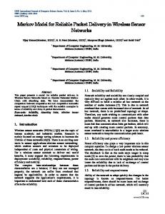
For d(i,j) < Rcorr , Kϑ {ksi − sj k} ≥ ξ. If any node nk is lying within Rcorr from node ni , it is within a strongly correlated distance from ni . Otherwise, the correlation is weak. The value of ξ can be determined according to the requirements of the application i.e., data resolution with desired reliability at the sink. A larger value of ξ implies stronger correlation. For the given parameters ϑ and ξ, a densely deployed WSN can be partitioned into disjoint clusters of size Rcorr . The cluster identification is basically the clique-covering problem over correlation graph, which is NP-hard [23]. A correlation graph G can be created where each node is represented by vertex, and edge (u, v) is drawn if the value of ρ(u,v) between node u and v is greater than or equal to ξ. As long as the correlation threshold ξ and the correlation function Kϑ (.) are given, the sets of correlated clusters are determined through a hierarchical clustering process. Details of this algorithm are presented in the appendix A.

4.2

Correlation based Energy-efficient Data Collection

According to the discussion in previous subsection, when a greedy correlated clustering algorithm is used, sets of correlated clusters are formed and all nodes in a cluster are considered highly correlated. The information is observed by multiple sensor nodes in the event area creating redundant reports. This can be eliminated by exploiting spatial correlation. Only a few nodes need to report their sensory data, and the remaining nodes can remain in a silent state to save energy. The best way to make the proposed correlation model work is to partition the entire event area into correlated, disjoint and equal-sized hexagons with radius Rcorr . By exploiting redundancy in sensor observations within correlated cluster, saving of energy is possible at the network layer. Since all the nodes in a cluster can be treated equally and only a small fraction of nodes (or at least one node) are allowed to be active to serve as the representative(s) of the whole cluster. The remaining nodes in the cluster can be kept in the sleep state. Thus network lifetime can be increased when nodes within a cluster share the workload. Since all the nodes in each correlated cluster most likely observe the same event information, it is desirable to schedule only one node at a time to pass on that information to the sink, in order to save energy within the cluster. Within each cluster, TDMA scheme can be implemented to assign different time slots to each node that will schedule the work sequentially in a cluster. A round-robin scheduling method can be adopted in the clusters [13]. For a cluster with k sensor nodes, the period T can be divided into k time slots. In every T time duration, every sensor node will work only for a Tk time period. Initially, the sensor nodes should be time synchronized, and then the sink node can randomly assign a working schedule to the sensor nodes for each cluster. We simulated the correlation-based clustering using the proposed Algorithm-I (appendix A) by placing 60 nodes with a sensing range of 20 meters for different values of ξ. The results are shown in Fig. 4. It is clearly seen that the number of correlated clusters and the number of member nodes in a cluster depend on the value of the correlation threshold ξ. If ξ is smaller a larger number of nodes falls in a correlated cluster on an average. On the other hand, a larger value of ξ allows a lesser number of correlated nodes in a cluster. Similarly, for different values of ϑ with fixed node density, the sensor network is partitioned into different-sized correlated regions. Hence, the required information reliability/fidelity can be achieved through proper clustering by

+ The copy of record is available at IET Digital Library.

Correlation Model

11

Table 2: Results of Rcorr PP ξ PP 0.2 ϑ (m.) PPP P 9 5.78 12 8.03 15 10.04 18 12.07 21 14.0 24 16.13

for different values of ϑ and ξ 0.4

0.5

0.6

0.8

4.11 5.5 6.23 8.23 9.6 11.07

3.51 4.7 5.87 7.05 8.23 9.39

2.3 3.05 3.86 4.67 5.44 6.22

1.25 1.7 2.16 2.59 3.02 3.46

180

180 160

160 140

140

120

120

100 y (meters)

y (meters)

100

80

60

80

60

40

40

20

20

0

0

−20 −20

0

20

40

60

80 x (meters)

100

120

140

160

180

−20 −20

0

20

40

60

(a)

80 x (meters)

100

120

(b)

Figure 4: Correlation-based clustering results using Algorithm-I for 150 sensor nodes with θ1 = 40 m for (a) ξ = 0.25 and (b) ξ = 0.5.

controlling parameters ϑ and ξ in data collection. Table 2 shows the results of Rcorr for different values of ϑ and ξ. The event area observed by the sensor nodes might change due to a change in environmental conditions. In this case, based on the reliability requirements, the sink node should decide whether the current clusters are valid or not. Then it should re-adjusts the clusters as quickly as possible by tuning the parameters ϑ and ξ and re-executing Algorithm-I. Thus, data reliability can be improved by re-partitioning of the whole network.

5

Exploiting the spatial correlation at MAC layer

Several MAC protocols have been proposed to take advantage of spatial correlation. Some of them have been analysed in [1], [2], [3] and [15]. In this section, we first present a framework, using our correlation model to compute estimation error in terms of event distortion. Here, our

+ The copy of record is available at IET Digital Library.

140

160

180

Correlation Model

12

objective is to choose the minimum number of nodes inside the event area such that the final achieved event distortion is within the tolerable distortion constraints. A comparative case study has also been presented with the existing models.

5.1

WSN Model

Consider a WSN, where N sensor nodes are evenly distributed over a measurement field D (D ⊂ R2 ). The event source S occurs inside the field D and is located in the center of the event area. The nodes falling in the event area will have threshold exceeded (called reporting nodes) and thus send the sensory information to the sink. The WSN should be designed to minimize mean square error (MSE) distortion between event source S and its estimation Sˆ from the sensors’ collective observations. The MSE distortion of the event is defined as a reliability measure required by the sensor applications. It is given as ˆ DE = E[dE (S, S)].

(10)

ˆ is the event MSE distortion measure and E(.) represents mathematical expectation. Here dE (S, S) In this paper, we refer Dmax as the maximum tolerable information distortion allowed in the sensor network as per the application requirement. The sink reconstructs an estimate of the event source by exploiting the spatial data correlation while ensuring given distortion constraint Dmax (i.e., DE ≤ Dmax ). A simple Gaussian sensor network is considered as Gaussian distribution usually have maximum entropy. We assume that an event can happen anywhere in the field, denoted by event source S. The event source S can be modeled as a random process s(t, x, y) at a time t and spatial coordinate (x, y). We can approximately estimate the (x, y) as centroid of all the reporting nodes. The weighted average of the information sensed by all the reporting nodes will give the ˆ We also assume that N nodes sense the event and send the information to the sink. estimate S. Let a node ni observes the event S as Si . Due to noise and other imperfections, the sensed data will be Xi . The node ni encodes Xi and transmits it to the sink through multi-hop transmission. The sink node decodes all the received Xi ’s to estimate the Si ’s. The encoder and decoder are denoted by E and D respectively as shown in Fig. 5. The variance of event information Xi is assumed to be same as variance of event source S. After collecting the event information Xi from node ni , the sink estimates values of event information using the best estimator. As the sensor nodes send the event information only when it is above a threshold, the mean value of data received from the reporting nodes is expected to be above threshold. As Fig. 5 shows, once the event of interest happens, node ni observes the signal Xi with noise, at time t. Since the samples are temporally independent, we neglect the time index t. Xi = Si + Ni ;

i ∈ N.

(11)

Here, measured information Xi is assumed to be Jointly Gaussian Random Variable (JGRV) and 2 Ni is zero mean Gaussian noise with variance σN . Hence, E[Si ] = mi ,

Var[Si ] = σS2 ,

and ρ(i,j) = Kϑ (d(i,j) ) =

2 Var[Ni ] = σN , i = 1, 2, ...N,

E[(Si − mi )(Sj − mj )] . σS2

(12)

Here ρ(i,j) is the correlation coefficient between nodes ni and nj located at coordinates si and sj . The d(i,j) is the distance between these nodes and Var(.) represents mathematical variance. The function Kϑ (.) can be determined using the correlation model discussed in the earlier section. + The copy of record is available at IET Digital Library.

Correlation Model

13

Figure 5: WSN Model for Event Source S estimation

In the literature, Spherical, Power exponential, Rational quadratic, and Matérn [20] correlation models have also been proposed. For the case of sensor network with omni-directional sensor nodes, these conventional models do not consider the real network conditions such as sensing range, location of nodes, and distance between nodes etc.. Our proposed model first needs the coordinates of node placements and sensing range. While the earlier proposed ones do not use these parameters. It should be noted that when node placement and sensing range are unknown, our model cannot be used. Therefore, the correlation models must be chosen according to the properties of the physical phenomena and the sensed events’ features. The events’ features vary significantly for the energy-radiating physical phenomenon originating in the field. In this paper, we have considered those events which trigger all the nodes within a radius of sensing range. They do not trigger the nodes which are out of range irrespective of value of S. Assume, S represents energy-radiating signal that propagates. The signal strength of event source S decays with distance and it follows isotropic attenuation power model, given by Si =

S0 , 1 + βdα i

(13)

where S0 is signal strength of event source, β is constant, and di is Euclidean distance between the node ni and event source. The signal attenuation exponent is represented by α ranging from 2 to 3. For simplicity, we use β = 1 and α = 2. Since we have used average of sensed information by all the reporting nodes, the estimated value Sˆavg will be smaller than actual S. Let us assume that an event S triggers N reporting nodes within event radius RE and Sˆavg will be average of ˆ all the measured event information Sˆi from all these √ N nodes. Let this Savg be equal to decayed version of S at a distance of Rc (where Rc = RE / 2). Since we have used a simpler approach, Sˆi , ∀i, is estimated using MMSE at the sink. Using Sˆi , Sˆavg is estimated, which is further scaled up to get Sˆ by a factor obtained from (13) for di = Rc . It should be noted that the estimation Sˆi , ∀i, is also a JGRV with same properties, as the actual event information Si , ∀i, is a JGRV. The sink will receive N measured values, as sample observations from N reporting nodes as given by X = AZ + W. N ×1

(14) N ×1

Here, the vector, X ∈ R is sample observation, Z ∈ R is random vector for physically sensed event information, A ∈ RN ×N is known transformation matrix and W ∈ RN ×1 represents noise vector. For simplicity, A is taken as identity matrix. Here R is the set of real numbers.

+ The copy of record is available at IET Digital Library.

Correlation Model

14

We also have T

E[Z] = [m1 , m2 , . . ., mN ] ∈ RN ×1 , where



Css

Cov[Z] = Rzz = σs2 Css ∈ RN ×N ,

ρ(1,1)  ρ(2,1)  = .  ..

ρ(1,2) ρ(2,2) .. .

··· ··· .. .

 ρ(1,N ) ρ(2,N )   ..  . . 

ρ(N,1)

ρ(N,2)

···

ρ(N,N )

(15)

(16)

The elements of correlation matrix Css is defined by our proposed correlation model (6). The ˆ of Z can be formulated using the affine function [21] of X as MMSE estimate, Z ˆ = KX + b, Z

(17)

where K is a matrix and b is a vector. It minimizes the scalar MSE criterion. According to ˆ will be a MMSE estimate if E[(Z − Z)] ˆ = 0 and E[(Z − Z)X ˆ T ] = 0. orthogonality principle [21], Z Thus, we have −1 2 (18) IN ) . b = E[Z] − KE[X], K = Rzz (Rzz + σN Using (14), (15) and (18), (17) can be simplified as 2 ˆ = E[Z] + Css (Css + σN IN ) Z σS2

−1

¡

X − E[X]

¢

.

(19)

The error covariance matrix, Ree can be calculated as ˆ ˆ T ] = Rzz − Rzz (Rzz + σ 2 IN )−1 Rzz = (Rzz −1 + σ 2 IN )−1 , Ree = E[(Z − Z)(Z − Z) N N

(20)

−1

where, second quantity is obtained using an identity A-1 + A-1 C(D − BA-1 C) BA-1 = −1 (A − CD-1 B) [22]. ˆ = [Sˆ1 , Sˆ2 , . . ., SˆN ]T ∈ RN ×1 . The estimated values, Sˆi ’s are spatially correlated because Here Z the observed event information Xi ’s are spatially correlated. The too-much redundancy in data is not needed once the estimates is within distortion constraint (denoted by Dmax ) as decided by application requirement. If somehow, only a subset of nodes is allowed to transmit, it will be good enough to meet this constraint Dmax . Therefore, we investigate the achieved distortion when only M out of N nodes are selected to send event information to the sink. Since the ˆ the estimate estimator uses the average of estimate Sˆi with scaled version obtained from (13), S, of S is given as M

2 X T (1 + Rc2 ) ˆ ) = (1 + Rc ) S(M Sˆi = [1, 1, . . ., 1][Sˆ1 , Sˆ2 , . . ., SˆM ] . M M i=1

(21)

The event distortion achieved by selecting M packets, when each reporting node transmits only one report to the sink, can be estimated from average value of sensed information. The achieved (1+R2 ) event distortion DE is calculated as MSE [21, 22] that is equal to M 2 c trace(Ree ) using (20) and (21). Here trace(A) is the trace of the matrix A. The calculation of distortion DE (N, M ) can be simplified by selecting M nodes (M < N ) through vector expansion in an alternative form as h¡ ¢ i ˆ ) 2 . DE (N, M ) = E S(N ) − S(M (22) + The copy of record is available at IET Digital Library.

Correlation Model

15

For fixed values, RE = 10 m., θ = 20 m. 1400 Ntot = 625, N = 489, λ = 1.56 (Random Selection) Ntot = 400, N = 316, λ = 1.0 (Ordered Selection [16]) Ntot = 400, N = 316, λ = 1.0 (Random Selection) N

tot

1000

0.9

= 100, N = 80, λ = 0.25 (Random Selection) 0.8 Correlation Coefficient ρ

Observed Event Distortion DE

1200

800

600

ρ = 0.39 ρ = 0.68

400

ρ = 0.75

0.7 0.6 0.5 0.4 0.3 0.2

200

0.1

0 0

0.2 0.4 0.6 0.8 Ratio of selected nodes to total nodes (M/N)

1

0

2

4 6 Node density λ

(a)

8

10

(b)

Figure 6: (a) The average distortion for different λ values according to changing the number of selected nodes in the event area. (b) The change of correlation coefficient with node density λ for fixed θ = 4 m in grid topology.

Expanding (22) using (11), (12) and (21), 2

DE (N, M ) =

(1 + Rc2 ) NM −2

N P i=1

· N σs2 + PM

j=1 j6=i

N P i=1

m2i +

mi mj +

σs2

M P i=1 N P

m2i − PN

i=1

j=1 j6=i

σs4 2 ) (σs2 + σN ρ(i,j) +

µ

N P P M

2

j=1 j6=i

i=1

σs6

¶ ρ(i,j) − M

M P P M 2

2 ) (σs2 + σN

i=1

j=1 j6=i

#

(23)

ρ(i,j) .

Here the correlation coefficients ρ(i,j) are the elements of correlation matrix Css which takes into account of sensing range and node separation. Using this distortion function, a case study has been presented in the next section.

5.2

Case studies for Reconstruction performance

The achieved event distortion at the sink is computed using (23) which is the function of N reporting nodes, the correlation matrix Css and Rc , while other parameters are constants such as M , mi , σS , σN . In section 5.2.1, we study the impacts of node density, selected node number and sensing range (where r = ϑ/2) on the distortion performance using (23). As discussed in section 3.3, the achieved distortion strongly depends on the correlation coefficient, ρ(i,j) . In this case, the location of event source is not a necessary requirement. Unlike existing models [2, 3], our model does not need actual location of event source and thus will be more suitable for real network scenarios. A comparative study has also been provided in section 5.2.2 to investigate the impacts of correlation coefficients on distortion performance. We extend the work of [2] and [3] using an alternative event driven sensing model and a new correlation function.

+ The copy of record is available at IET Digital Library.

Correlation Model

5.2.1

16

Case-1: Impacts of node density and selected node number on distortion

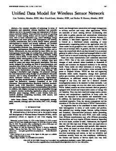
In this subsection, the impacts of node density and number of node selection on √ √ the reliability of event estimation at sink are studied. We conduct simulations over Ntot d × Ntot d m2 grid area where Ntot sensor nodes are located on the grid. The node density λ, as the number of nodes per unit area is d12 . We place an event source in the center of grid area where N nodes are activated within the event radius RE . The simulations are performed with 1000 trails and the results are produced by averaging them as shown in Figs. 6 and 7. Fig. 6(a) shows the results of the event distortion for different values of node density λ according to changing the number of selected nodes with respect to total reporting nodes (i.e., the ratio of total selected nodes to total reporting nodes) for a given event area. It is observed that the distortion approaches to relative by constant value when the reporting nodes (i.e., M ) are more than a threshold percentage of total nodes sensing the event (i.e., N ). We have chosen the reporting nodes such that they should be as closer as possible to center of area where N nodes have sensed the information, while the reporting nodes are as far as possible from each other [17]. When node density λ increases, the spatial correlation coefficient also increases for fixed value of ϑ as shown in Fig. 6(b). It means that a higher node density indicates a stronger correlation among data sample which resulting a better estimation reliability. Hence, the event distortion also becomes a monotonically decreasing function of λ as shown in Fig. 6(a). On given 0.25 node density, 20% of total reporting nodes are sufficient to be activated for event reporting. This further implies that optimum performance can be achieved by allowing lesser number of reporting nodes M to be activated in the event area (M < N ). Thus, the energy can be saved by exploiting spatial data correlation to limit the reporting nodes while ensuring acceptable distortion constraint Dmax . Fig. 7 shows the results of the M reporting nodes for different values of correlation coefficient ρ when the observed event distortion does not exceed Dmax at the sink. Minimum Number of Nodes for D

= 2000, R = 15 m

max

E

2500 M reporting nodes N reporting nodes Node size in event area

2000

1500

1000

500

0

0.07 0.24 0.36 0.48 0.53 0.59 0.62 0.65 0.69 0.72 0.75 0.78 0.81 0.84 0.87 Correlation Coefficient ρ ( function of λ node density )

Figure 7: Optimal value of Nmin reporting nodes with different correlation coefficients ρ.

5.2.2

Case-2: A comparative study

In the research work reported in [2] and [3], a simple correlation model has been used for computing distortion in event reconstruction. Using this model, the expressions of distortion are derived to find the minimum number of representative nodes, M , out of total N nodes inside the event + The copy of record is available at IET Digital Library.

Correlation Model

70

θ =500, Vuran and Akyildiz [2] θ = 5000, Vuran and Akyildiz [2] θ1 = 40, our Method

60

θ = 20, our Method

1.8

2

50 40 30 20 10 0

α = 0.1, Zheng and Tang [3] θ1 = 40, our Method

1.6 Observed Event Distortion

Observed Event Distortion

80

17

θ = 20, our Method 2

1.4 1.2 1 0.8 0.6

10

20 30 40 50 Number of representative nodes

60

70

(a)

0.4 0

10

20 30 40 50 Number of representative nodes

60

70

(b)

Figure 8: Comparison of average event distortion performance using (a) our method and the work of Vuran and Akyildiz [2], (b) our method and the work of Zheng and Tang [3].

area. The minimum number M is needed to report data without exceeding the tolerable distortion constraint. Using the same expressions and assumptions as in [2, 3], we extend the work by applying our correlation model for the purpose of computing event distortion. In [2] and [3], the Power exponential model [20] is used as the correlation model to compute the event distortion. For same expressions of distortion, we use our proposed more realistic correlation model given by (6). To gain more insight into event reconstruction distortion using our correlation model, we conduct a comparative analysis with the methods suggested in [2] and [3] respectively. In a 1000 × 1000 m2 grid area, we have deployed 70 nodes randomly and a fixed event source in the center of the grid area. The event reconstruction distortion has been calculated over a range of 0−70 sensor nodes that are sending event information to the sink. The simulation was performed using a fixed topology with 1000 trials. The event distortion was evaluated using our and existing correlation models. These results are plotted in Fig. 8. Fig. 8(a) shows a comparison of results obtained by methodology of [2] using Power Exponential model and our correlation model. For the given total N nodes, the distortion decreases logically with the increase in M representative nodes that are activated to send event information. This happens as more event information is received at the sink with larger M . However, using our model, at the same number of M representative nodes, even lesser distortion is achieved (see Table 3). It is shown that achieved distortion can be preserved at the sink using our model by allowing Nmin nodes (< M ) to be active. If somehow, only selected Nmin nodes transmit event information, we can reduce the energy consumption. Fig. 8(b) shows a comparison using the method suggested in [3], between the earlier model and our model. It indicates the same behaviour, that reduced achieved distortion allows a lower value of Nmin which is less than M . Hence, using our correlation model, energy consumption in data transmissions and collisions can be minimized at the MAC layer. Furthermore, the observed event distortion decreases with decreasing sensing range as shown in Figs. 6 and 8. To illustrate this, we can have a predefined Dmax value as allowed by the sensor network application. The results obtained, (Table 3) shows that for the minimum Dmax , θ1 has to be 10 m while for higher Dmax , θ2 can be 111 m for same Nmin (i.e., 15) representative nodes.

+ The copy of record is available at IET Digital Library.

Correlation Model

Table 3: Results of ϑ for different values XX XXX Dmax XXX 22 24 26 Nmin XX 15 10 28 49 17 18 36 58 19 26 47 67 21 38 58 77 23 47 69 89 25 54 74 98

18

of Nmin and Dmax 28

30

32

69 80 89 97 108 116

87 99 110 119 128 137

111 118 127 139 148 157

Higher θ2 implies that less number of nodes are used in same field. Hence, for same Nmin nodes and lesser distortion Dmax , the sensing range of the nodes needs to be kept small through the control parameter (i.e. ϑ). Consequently, we can state based on our correlation model that the power consumption can be minimized by somehow allowing smaller number of nodes to report the event while attaining the desired event reliability as specified by Dmax . Both Fig. 8(a) and Fig. 8(b) indicate a lower bound on the minimum number of representative nodes that need to send the event information based on our correlation model.

6

Conclusion

In this paper, a basic correlation model has been introduced to represent the correlation characteristics between sensor nodes. Using the proposed correlation model, various key elements discussed at both Network and MAC layer. We found that the densely deployed WSN can be partitioned into non-overlapping correlated regions at network layer. Thus, only single node needs to be allowed to report data rather than every node from a given correlated region, resulting in significant energy savings during data collection. Furthermore, our results show that required event reliability can be achieved through proper tuning of ϑ and ξ, i.e., both the sensing range and the correlation threshold for reliable data delivery. In the context of MAC, we have investigated the impacts of node density, number of selected nodes and nodes’ sensing range on the achieved event distortion at the sink. For the estimation of event source, the optimum node density within an event area can be found at minimum observed event distortion. In addition, a comparative study showed that the proposed correlation model outperforms existing correlation models. We observed that optimal value of Nmin nodes can be achieved through proper tuning of ϑ for given Dmax as per application requirement. In this context, we also conclude that our approach takes into account the node location and sensing range. Most of the redundant transmissions can be filtered out on the basis of presented model to make a more energy-efficient MAC design for sensor network applications.

A

Appendix

The flow chart of Greedy Correlated Clustering Algorithm is shown in Fig. 9.

+ The copy of record is available at IET Digital Library.

Correlation Model

19

Start

k = 0

Find most correlated pair nodes,

ni

and

nj among unclustered nodes ρ(i,j) has largest value)

(i.e.,

No If

ρ(i,j)

>

ξ

?

Yes Make cluster by adding as

ni , nj

Ck = {ni, nj }.

nl from unclustered nodes such that least value of correlation (i.e., ρ(.)) with

Find a node

member nodes of

Ck

nl exists ρ(l,k)>ξ ?

If any and

nl Ck

Add

is maximum.

to

Yes

k =k+1 No

If unclustered nodes are there ?

Yes

No

Stop

Figure 9: Flow chart of Greedy Correlated Clustering Algorithm

+ The copy of record is available at IET Digital Library.

Correlation Model

20

References [1] Vuran, M.C., Akan, O.B., and Akyildiz, I.F.: ‘Spatio-temporal correlation: theory and applications for wireless sensor networks’, Comput. Netw. J. (Elsevier), vol. 45, 2004, pp. 245–259 [2] Vuran, M.C., and Akyildiz, I.F.: ‘Spatial Correlation based Collaborative Medium Access Control in Wireless Sensor Networks’, In IEEE/ACM Trans. On Networking, vol. 14, no. 2, 2006, pp. 316–329 [3] Zheng, G., and Tang, S.: ‘Spatial Correlation-Based MAC Protocol for Event-Driven Wireless Sensor Networks’, In Journal of Networks, vol. 6, no. 1, Jan 2011, pp. 121–128 [4] Akyildiz I.F., and Vuran, M.C.: ‘Wireless Sensor Networks’ (John Wiley & Sons, 2010) [5] Scaglione, A., and Servetto, S.: ‘On the interdependence of routing and data compression in multi-hop sensor networks’, Wireless Networks (Elsevier), 2005, pp. 149–160 [6] Yoon, S., and Shahabi, C.: ‘Exploiting spatial correlation towards an energy efficient clustered aggregation technique (CAG)’, In Proc. of ICC,05, Seoul, Korea, vol. 5, 2005, pp. 3307–3313 [7] Pattem, S., Krishnmachari, B., and Govindan, R.: ‘The impact of spatial correlation on routing with compression in wireless sensor networks’, In Proc. of IPSN,04, Berkeley, California, USA, 2004, pp. 28–35 [8] Li Na, Liu Yuanan Wu Fan, and Tang Bihua: ‘WSN Data Distortion Analysis and Correlation Model Based on Spatial Locations’, In Journal of Networks, vol. 5, no. 12, Dec 2010, pp. 1442–1449 [9] Pradhan, S.S., Kusuma, J., and Ramchandran, K.: ‘Distributed Compression in a Dense Microsensor Network’, IEEE Signal Processing Magazine, Vol. 19, No. 2, 2002, pp. 51–60 [10] Zahraie, M.S., Farkhady, A.Z., and Haghighat, A.T.: ‘Increasing Network Lifetime by Optimum Placement of Sensors in Wireless Sensor Networks’, Computer Modelling and Simulation, 2009. UKSIM ’09. 11th International Conference on, March 2009, pp. 611-616 [11] Xiao, Y., Chen, H., Wu, K., Sun, B., Zhang, Y., Sun, X., and Liu, C.: ‘Coverage and detection of a randomized scheduling algorithm in wireless sensor networks’, IEEE Trans. Comput., vol. 59, no. 4, 2010, pp. 507–521 [12] Tezcan, N., and Wang, W.: ‘TTS: a two-tiered scheduling mechanism for energy conservation in wireless sensor networks’, International Journal of Sensor Networks, vol. 1, no. 3, Jan 2006, pp. 213–228 [13] Liu, C., Wu, K., and Pei, J.: ‘A Dynamic Clustering and Scheduling Approach to Energy Saving in Data Collection from Wireless Sensor Networks’, Proc. Second IEEE Int’l Conf. Sensor and Ad Hoc Comm. and Networks, Sept. 2005 [14] Dong, M., Tong, L., and Sadler, B.: ‘Impact of data retrieval pattern on homogeneous signal field reconstruction in dense sensor networks’, Signal Processing, IEEE Transactions on, vol. 54, no. 11, Nov. 2006, pp. 4352–4364 [15] Zhao, M., Chen, Z., Zhang, L., and Ge, Z.: ‘HS-Sift: hybrid spatial correlation-based medium access control for event-driven sensor networks’, Communications, IET, vol. 1, no. 6, Dec. 2007, pp. 1126–1132 + The copy of record is available at IET Digital Library.

Correlation Model

21

[16] Shakya, R.K., Singh, Y.N., and Verma, N.K.: ‘A Novel Spatial Correlation Model for Wireless Sensor Network Applications’, Proc. of Ninth IEEE International Conference on wireless and Optical communications Networks (WOCN’2012), Sept. 2012, pp. 1–6 [17] Shakya, R.K., Singh, Y.N., and Verma, N.K.: ‘A Correlation Model for MAC protocols in Event-driven Wireless Sensor Networks’, Proc. of 2012 IEEE Region 10 conference, (TENCON 2012), Nov. 2012, pp. 1–6 [18] Ghosh, A., and Das, S.K.: ‘Coverage and connectivity issues in wireless sensor networks: A survey’, Pervasive and Mobile Computing Vol. 4, No. 3, 2008, pp. 303–334 [19] Guvensan, M.A., and Yavuz, A.G.: ‘On coverage issues in directional sensor networks: A survey’, Elsevier Ad Hoc Networks, Vol. 9, Issue 7, Sept. 2011, pp. 1238–1255 [20] Berger, J.O., de Oliviera, V., and Sanso, B.: ‘Objective bayesian analysis of spatially correlated data’, J. Am. Statist. Assoc.96, 2001, pp. 1361–1374 [21] Kay, S.M.: ‘Fundamentals of Statistical Signal Processing, Vol. I: Estimation Theory’, Prentice-Hall, 1993 [22] Bhatia, R.: ‘Matrix Analysis’, New York:Springer-Verlag, Graduate Texts in Mathematics, Vol.169,1991 [23] Garey, M.R., and Johnson, D.S.: ‘Computers and Intractability; A Guide to the Theory of NP-Completeness’, (New York, NY, USA: W.H. Freeman & Co., 1990)

+ The copy of record is available at IET Digital Library.

This paper is a postprint of a paper submitted to and accepted for publication in “IET Wireless Sensor Networks" and is subject to Institution of Engineering and Technology Copyright.

The copy of record is available at IET Digital Library.