some statistical re{interpretation of existing data. In- deed, it may be pro table ... Allan Poe, that there be lies, damned lies, and statis- tics! References. Angeline ...
Genetic Extensions of Neural Net Learning: Transfer Functions and Renormalisation Coe�cients Marc Schoenauer
Abstract This paper deals with technical issues relevant to arti cial neural net (ANN) training by genetic algorithms. Neural nets have applications ranging from perception to control; in the context of control, achieving great precision is more critical than in pattern recognition or classi cation tasks. In previous work, the authors have found that when employing genetic search to train a net, both precision and training speed can be greatly enhanced by an input renormalisation technique. In this paper we investigate the automatic tuning of such renormalisation coe�cients, as well as the tuning of the slopes of the transfer functions of the individual neurons in the net. Waiting time analysis is presented as an alternative to the classical "mean perfomance" interpretation of GA experiments. It is felt that it provides a more realistic evaluation of the real-world usefulness of a GA.
1 The Usefulness of Automatic Parameter Tuning The operator of a heuristic program spends a lot of time predicting what his program will do. Now and then a test run actually validates the programmer's prediction and life, science, and everything is wonderful { yet more often, the program goes o� to do its own thing and the programmer is left to scratch his head. In this context, manual tuning of parameters is one of the least rewarding facets of heuristic programming. For instance, the authors have spent hours in front of computer screens, when investigating neural net training. These hours were occupied by running the same program time and again with just the change of a single real parameter like the slope of the neural transfer function. Computer programming is of necessity experimental; however every worker in the eld of genetic algorithms has been brought to conjecture that the experimenter's action could be automated. In the case of GA research, the manual variation of GA parameters {eg. search for good mutation or crossover rates { could be replaced by the action of a meta-GA. Unfortunately, the computational expense of running a population of GA's in parallel usually discourages the
Edmund Ronald GA experimenter from pursuing such a course of automatic experimentation, although object-oriented software engineering makes a 2-level GA easily feasible. Indeed, the possibility of running a meta-GA is a design goal of the authors' next generation GA software. In the special case of the authors' research in neural net control, some of the parameters originally subject to tuning could be varied by the same GA employed to train the net by searching the space of weight matrices. In this document the results of this automated research is confronted with the results originally published in [Ronald & Schoenauer 93] . In summary, by confronting the results of our previous work with this automated tuning by GA, we show that the GA improves on a human operator in tuning some of the net parameters, namely the transfer functions. On the other hand, automatic renormalisation, as presented in section 5 does not improve mean precision, and indeed produces barely acceptable results; but it holds the promise of obsoleting the painful data pre-processing steps which hinder real-world and industrial applications of neural nets. We have included a waiting-time interpretation of our results; we believe that this interpretation methodology, while unusual, is more appropriate in an industrial context than mean performance: GAs are stochastic, and estimations of their performance must perforce be formulated in probabilistic terms. A waiting time estimation provides us with a con dence factor whereby a control problem can be solved with a predetermined amount of computation. The plan of the paper follows: In section 2 below we recall the neural net formalism and its application to control, and summarise earlier work. Section 3 presents an investigation into the automatic tuning of the neural transfer function slopes. Section 4 introduces the waiting time analysis, and applies it to the results of section 3. Section 5 describes experiments in generalised tuning of both data renormalisation coef cients and transfer functions. Section 6 discusses the signi cance of the results, and highlights some possible applications.
2 Genetic Training of Neural Net Controllers
Figure 1: Best non-normalised control action in study.
In order to make this paper self-contained, this section summarises the methods employed by the authors for neural net control in [Ronald & Schoenauer 93], [Schoenauer & Ronald 94]. This establishes the background for the numerical experiments on the lunar lander simulator, whose results form the body of sections 3 and 4 below. The reader desiring an overview of the eld may refer to [Yao 93], a broad survey of evolutionary methods as applied to neural net training and design.
A very nice lunar landing e�ected in this study is shown in Figure 1. This achieved a landing speed of 7 10?7m=s, ie. 0:7mm=s, hardly enough to mark the lunar surface! Such excellence would hardly be necessary in practice. This result was obtained by straightforward application of neuro-genetic control, with no data renormalization.
2.1 Lunar lander dynamics This paper deals with training a neural net to land a simulated rocket-driven lunar-lander module, under a gravity of 1.5 m=s2 . This simulation has given rise to numerous computer games since the advent of interactive computing, and will be familiar to most readers. The lunar module is dropped with no initial velocity from a height of 1000 meters. The fuel tank is assumed to contain 100 units of fuel. Burning one unit of fuel yields one unit of thrust. Maximum thrust is limited to 10 units and the variation of the mass of the lunar module due to fuel consumption is not taken into account. The simulation time-slice was arbitrarily xed at 0.5 seconds. All the experiments reported i this document were conducted with the given initial height; the net can be trained to solve the general control problem by the expedient of supplying random starting points. However such training was deemed too expensive computationnally to allow for the exhaustive experimentation whose results are reported here. The input parameters relayed to the neural net once every time-step are the speed, and the altitude. The net then computes the desired fraction of maximal thrust, on a scale from 0 to 1, which is then linearly rescaled between 0 and 10 units.
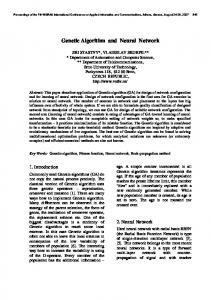
The best landing we achieved in this study is shown in Figure 1. The landing speed of 7 10?9m=s, ie. 0:002mm=s is a 2 orders of magnitude improvement over the previous result, and was attained in half as many (1035) generations. This is an achievement of data renormalisation: The net was presented with the two previously cited state inputs, namely speed and altitude, and another pair consisting of the same variables pre-multiplied by a factor of 10. Altitude -10*Speed 100*Thrust
1000
500
0
0
Altitude -10*Speed 100*Thrust
1000
It was attained at the price of a long run, namely almost 2000 generations. The control action is also exemplary in the economy of fuel in the deceleration phase: For the main deceleration burst, thrust is pulsed in what amounts to almost a square wave to its maximal permissible value. The remarkable landing softness is attained by means of a long - and very smooth- hover phase which begins immediately after deceleration.
10
20
30
40
50
60
Best 10-normalized net, gen. 1035, landing speed 2e-9 m/s
Figure 2: Best overall control action in study. 500
0
0
10
20
30
40
50
Best unnormalized net, gen. 1865, landing speed 7e-7 m/s
60
The interesting features of the best "Armstrong", as displayed in Figure 2, are its surprising precision, and the fact that this precision is attained either in spite of, or more probably, because of the displayed sawtooth shape and roughness of the thrust control. Of course, control by rocket to t a speed tolerance of 20 Angstroms/s seems rather implausible in reality.
2.2 The Networks A classical 3-layered net architecture was employed, with complete interconnection between layers 1 and 2, and 2 and 3. The neural transfer function (non-linear squashing) was chosen to be the usual logistic function F , a sigmoid de ned by F (x) = 1+e1?�x In our work the parameter � was xed, � = 3:0. Each individual neuron j computes the traditional [PDP] squashed sum-of-inputs
oj = F (
Pi wij xi )
Regarding the sizing of the middle layer, we chose to apply the Kolmogorov model [Hecht-Nieslen 90] which for a net with n inputs and 1 output requires at least 2n+1 intermediate neurons. Only two net architectures occur in this paper. Both types have only one output (controlling the lunar module's thrust). The canonical method for solving the control problem entails 2 inputs, namely speed and altitude, appropriately normalised between 0 and 1. However, the optimisation by input renormalisation which forms the core of Ronald entails adding two inputs to the above cited net, therefore employing 4-input nets. As in both cases we have adhered to the Kolmogorov paradigm, we are studying 2-51 and 4-9-1 nets, which respectively have 21 and 55 weights/biases. With the topology xed, training these nets for a given purpose is a search in a space of dimension 21 or 55, to which must be added real numbers representing the parameters �, and those for the renormalisation, when these parameters are left to the GA to nd. In the neuro-genetic approach, net training is thus a search in a 21 or 55-dimensional space, to which must be added real numbers representing the parameters �, and those for the renormalisation, when these parameters are left to the GA to nd.
2.3 The Genetic Model Our genetic algorithm software subjects a small population of nets to a crude parody of natural evolution. This arti cial evolutionary process aims to achieve nets which display a large tness. The tness is a positive real value which denotes how well a net does at its assigned task of landing the lunar module. Thus our tness will be greater for slower landing speeds. The details of the calculation of the tness are found below. For the purpose of applying the genetic algorithm, a net is canonically represented by its weights, i.e. as a vector of real numbers. During the initial stages of this work, two distinct homebrew GA software packages were employed. One package followed the rst methods presented by John Holland in that it uses bitstrings to encode oating-point numbers. The second software package, described below, was a hybridized GA which directly exploits the native oating-point
representation of the worktations which it was run on. The hybridization towards real numbers is described in [Radcli�e 91] and [Michalewicz 92]. The results obtained with both programs were consistent, and only the experiments with the oating point package are detailed in this document. The genetic algorithm progresses in discrete time steps called generations. At every generation the tness values of all the nets in the population are computed. Then a new population is derived from the old by applying the stochastic selection, crossover and mutation operators to the members of the old population. � Selection is an operator that discards the least t members of the population, and allows tter ones to reproduce. We use the roulette wheel selection procedure as described in [Goldberg 89], with tness scaling and elitism, carrying the best individual over from one generation to the next. � Crossover mixes the traits of two parents into two o�spring. In our case, random choice is made between two crossover operators: Exchange of the weights beteween parents, at random positions. Or assigning to some of the weights of each o�spring a random barycentric combination of its parents' weights. � Mutation randomly changes some weights by adding some gaussian noise. The experiments described in the next section used the following parameters in the GA: The net connection weights forming the object of the search were con ned to the interval [?10; +10] thereby avoiding over ow conditions in the computation of the exponential. Population size was held to 50 over the whole length of each run, tness scaling was set to a constant selecetive pressure of 2.0, crossover rate was 0.6, mutation rate 0.2, the gaussian noise had its standard deviation set to half the weight space diameter, ie. 10.0, decreasing geometrically in time by a factor 0.999 at each generation.
3 Adjusting Transfer Functions 3.1 The family of logistic transfer functions A great deal of work in the neural net community has employed logistic sigmoid transfer functions of the form F� (x) = 1 + 1e?�x where the parameter �, usually set to 1, can be seen to be de ning the slope of the function for x = 0, ie.
� = F� 0 (0)
1
102 Alphas == 3 Alphas in [0.5, 5] Alphas in [2,4]
101
Landing speed
In the gure below, we show the behaviour of F� for values of �, taken from the set f0:1; 0:5; 1:0; 2:0; 5g, with the slopes steepness increasing with � from a quasi-linear function, through a sigmoid to a very steep staircase.
100
10-1
10-2
Alpha = 0.1 Alpha = 0.5 Alpha = 1 Alpha = 2 Alpha = 5
10-3
0
500
1000
1500
2000
Generations
Fig 4. Mean performance with varying �
0.5
0 -10
-5
0
5
10
The family of logistic functions
In an analogy to biological systems, � can be interpreted as a chemical parameter de ning the sensitivity of a neuron. However, researchers in back-propagation usually x this parameter, although Yao, in his survey [Yao 93] cites Mani, as having experimented with a modi ed form of back-prop which performs gradient descent learning by adjusting the � slopes as well as the synaptic connection weights themselves. However, Yao also cites [Stork &al. 90] as having applied a GA approach to the de nition of both neural connectivity and transfer functions, an investigation similar to the one reported here.
3.2 Experimental Results In our case, we investigated how allowing a GA to individually tune the transfer functions a�ects the precision of control in the "genetic lander" experiment. Our results in allowing the GA to vary the � slope for each individual neuron in the controller net may be compared with work reported in [Ronald & Schoenauer 93], where the slopes of the transfer functions of all neurons were held constant at � = 3 .
In Figure 4 we have graphed the performance of the GA search, comparing the mean of a set of 60 1 runs of 2000 generations length with xed �, as reported in [Ronald & Schoenauer 93] with two new experiments of identical size. In these new experiments the GA was permitted to adjust the slope of each neuron, within the limits indicated in the gure. It can be seen that the mean maximum precision of the runs greatly improves when the GA is allowed to search a larger range of � slopes. The computational cost involves adding just one degrees of freedom per intermediate and output layer neuron, and can thus be considered negligible. In summary, we nd the technique of varying the slopes fully successful here, and we believe it deserves to be investigated in other contexts.
4 Waiting Time Estimation In the real world, a user who wishes to exploit a GA for a given task is not interested in average performance over a number of runs { she may rather wish for an estimation of how much it will take to achieve a result of a given quality: Such a result is an acceptable solution to the control problem, which can be acted upon. Now, if we assume a really bizarre genetic algorithm which yields a very bad result eg a crash at 10 m/s for half the random seeds, and an excellent result eg. 10e3 m/s for the other half, then the average result is a 5 m/s crash! However, just a very few runs of the algorithm will usually yield one of the "good" controllers, capable of piloting a safe ight. We may wish to formalize the above reasoning by asking the following question like someone who must run the GA in batch processing: If I know that on average a runs yields an acceptable result with probability a, then how many runs N must I schedule in order to have probability p or more of nding a good 1
4 runs on each CPU of a 15 workstation computer farm
Numb. of 500-gen. runs to 99% confidence
In the above formula we my assume any desired base for the logarithm. Hence for instance in the example, with a =0.5, and p=0.001 we can approximate in our heads that p = 2e ? 10 , and hence N = ?10= ? 1 = 10 . The above reasoning allows us to exploit the results of our computer runs with the aim of graphing the con dence factors. In this way, we transformed the data of the runs illustrated in Fig 4 above, yielding the graphs of Fig 5: Alpha in [0.5,5] Alpha in [2,4] Alpha == 3 100
50
0
-7
10
-6
10
-5
10
-4
10
-3
10
-2
10
-1
10
0
10
1
10
Required precision
Fig 5. Waiting time estimation with varying �
the search of renormalisation coe�cients entirely to the GA to nd in an interval [1e ? 10; 1e + 10]. However, these results may be considered less discouraging when the reader is told that the inputs for "full genetic renormalisation" were not preprocessed in any way! Thus the neural net, as trained by the GA, was left to deal with input values of eg. starting altitudes of 1000 m/s and free-fall speeds to 500 m/s, whereas in all other experiments neural input data had been folded (by hard code) into [0; 1]. Hence the "full genetic renormalisation" results are still promising - they yield a case of functional albeit imprecise control, as might be exploited by a prototype application. However such a prototype is obtained without any human expertise whatsoever being applied in the problem-domain. In this way one might imagine this "full genetic renormalisation" experiment to represent an industrial context, in which a feasibility study would be done for GA learning, without any prior attempt at data pre-processing. The authors would not believe their lives in danger even if landing is e�ected at 10 cm/s which the graph shows the GA-trained nets routinely achieve. Of course, a hand{tuned net able to land at 10e-7 m/s or so, would be more appropriate for piloting the director of a funding agency visiting a scienti c lunar base. Nber of 500-gen. runs to 99% confidence
run in the schedules runs? Elementary probability theory tells us that the con dence number N(p,n) is given by the equation N (p; n) >= log(p)=log(1 ? a)
2-inputs 4 inputs - Fixed renorm. 4 inputs - Guided genetic renorm. 4 inputs - Full genetic renorm.
100
50
The results of comparing the graphs in Figures 4 and 5 { created from the same experimental data { are nothing short of amazing! When we peer at gure 4, the mean landing speed of the 60 runs of 2000 generations' duration never reaches 10e ? 3. The waiting time graph in gure 4 however tells us that 10e ? 3 is a soft landing which we can reach with a con dence factor of 99% by e�ecting just 10 runs of 500 generations Fig 6. Waiting time estimation with varying � and renormalisations duration! The waiting time graph can be interpreted as showing that precisions of 10e ? 4 are perfectly attainable in practice with any of the investigated learning methods, be it manual or automatic tuning of the 6 Discussion slopes. 0
-7
10
-6
10
-5
10
-4
10
-3
10
-2
10
-1
10
0
10
1
10
Required precision
5 Generalised Tuning In gure 6 below we have reproduced the waiting time graph obtained from 4 experimental batches of 60 runs each, with and without GA search for input renormalisation coe cients. It can be seen that having no renormalisation at all is better than leaving
The results of the numerical experiments reported in this paper are mixed. On the one hand our data indicates that the slopes of the neural transfer functions can be pro tably trained by the same GA which trains the net. On the other hand the experiments on training renormalisation coe�cients by GA proved surprisingly disappointing, and will be investigated further. This should be contrasted with past experiments in which tuning these coe�cients by hand yielded excellent results.
The waiting time metric which we in introduced in section 3 above seems more suited to the logic of industrial application of GA control than the more conventional mean performance metric. Moreover, the counter-intuitive nature of this metric might inspire some statistical re{interpretation of existing data. Indeed, it may be pro table to unearth old experiments, deemed failures by the mean tness method, and reevaluate them. Let us remember the dictum of Edgar Allan Poe, that there be lies, damned lies, and statistics!
References [Angeline, Saunders & Pollack 94] P. J. Angeline, G. M. Saunders and J. B. Pollack, An evolutionnary algorithm that construct recurrent neural networks. To appear in IEEE Transactions on Neural Networks. [Goldberg 89] D. E. Goldberg, Genetic algorithms in search, optimization and machine learning, Addison Wesley, 1989. [Harp & Samad 91] S. A. Harp and T. Samad, Genetic synthesis of neural network architecture, in Handbook of Genetic Algorithms, L. Davis Ed., Van Nostrand Reinhold, New York, 1991. [Hecht-Nieslen 90] R. Hecht-Nielsen, Neurocomputing, Addison Wesley, 1990. [Holland 75] J. Holland, Adaptation in natural and arti cial systems, University of Michigan Press, Ann Harbor, 1975. [Kitano 90] Empirical studies on the speed of convergence of neural network training using genetic algorithms. In Proceedings of Eight National Conference on Arti cial Intelligence, AAAI-90, Vol. 2, pp 789-795, Boston, MA, 29 July - 3 Aug 1990. MIT Press, Cambridge, MA. [Mani ] G. Mani, Learning by Gradient Descent in Function Space, in Proceedings of IEEE Conference on System, Man, and Cybernetics, pp. 242247, Los Angeles 1990. [Michalewicz 92] Z. Michalewicz, Genetic Algorithms + Data Structures = Evolution Programs, Springer Verlag 1992. [Nguyen & Widrow 90] D. Nguyen, B. Widrow, The truck Backer Upper: An example of self learning in neural networks, in Neural networks for Control, W. T. Miller III, R. S. Sutton, P. J. Werbos eds, The MIT Press, Cambridge MA, 1990. [Radcli�e 91] N. J. Radcli�e, Equivalence Class Analysis of Genetic Algorithms, in Complex Systems 5, pp 183-205, 1991.
[Ronald & Schoenauer 93] E. Ronald, M. Schoenauer Genetic lander: An experiment in accurate neurogenetic control, in PPSN 94, to appear. [PDP] D. E. Rumelhart, J. L. McClelland, Parallel Distributed Processing - Exploration in the micro structure of cognition, MIT Press, Cambridge MA, 1986. [Scha�er, Caruana & Eshelman 1990] J. D. Scha�er, R. A. Caruana and L. J. Eshelman, Using genetic search to exploit the emergent behaviour of neural networks, Physica D 42 (1990), pp244-248. [Schoenauer & Ronald 93] M. Schoenauer, E.Ronald S.Damour, Evolving Networks for Control, in Neuronimes 93 , EC2, Paris 1993. [Schoenauer & Ronald 94] M. Schoenauer, E.Ronald Neuro Genetic Truck Backer-Upper Controller, in IEEE World Conference on Computational Intelligence , Orlando 1994. [Stork &al. 90] D. G. Stork, S. Walker, M. Burns & B. Jackson, Preadaptation in Neural Circuits, in Proceedings of International Joint Conference on Neural Networks 8, pp I-202{1-205, Erlbaum, Hillsdale 1990. [Yao 93] Xin Yao, A Review of Evolutionary Arti cial Neural Networks, in International Journal of Intelligent Systems 8, pp 539-567, 1993.