THE JOURNAL OF CHEMICAL PHYSICS 122, 124508 共2005兲
Geometry optimization of periodic systems using internal coordinates Tomáš Bučkoa兲 and Jürgen Hafner Computational Materials Science, Institut für Materialphysik, Universität Wien, Sensengasse 8/12, A-1090 Wien, Austria
János G. Ángyánb兲 Laboratoire de Cristallographie et de Modélisation des Matériaux Minéraux et Biologiques, UMR 7036, CNRS-Université Henri Poincaré, Boite Postale 239, F-54506 Vandœuvre-lès-Nancy, France
共Received 16 November 2004; accepted 11 January 2005; published online 30 March 2005兲 An algorithm is proposed for the structural optimization of periodic systems in internal 共chemical兲 coordinates. Internal coordinates may include in addition to the usual bond lengths, bond angles, out-of-plane and dihedral angles, various “lattice internal coordinates” such as cell edge lengths, cell angles, cell volume, etc. The coordinate transformations between Cartesian 共or fractional兲 and internal coordinates are performed by a generalized Wilson B-matrix, which in contrast to the previous formulation by Kudin et al. 关J. Chem. Phys. 114, 2919 共2001兲兴 includes the explicit dependence of the lattice parameters on the positions of all unit cell atoms. The performance of the method, including constrained optimizations, is demonstrated on several examples, such as layered and microporous materials 共gibbsite and chabazite兲 as well as the urea molecular crystal. The calculations used energies and forces from the ab initio density functional theory plane wave method in the projector-augmented wave formalism. © 2005 American Institute of Physics. 关DOI: 10.1063/1.1864932兴
I. INTRODUCTION
Recently, there has been an increasing interest in electronic structure calculations of three-dimensional periodic systems. Several high-performance density functional theory 共Refs. 1–5兲 and Hartree–Fock5,6 codes are available, permitting the study of structural features by gradient optimization. Until very recently, geometry relaxations in solids were done exclusively in terms of Cartesian and/or fractional coordinates, and lattice vector components.1,4,7–9 Although the Cartesian/fractional coordinates are simple and universally applicable, the use of internal 共atomic and lattice兲 coordinates as control parameters in geometry optimizations offer several advantages. As it has been extensively demonstrated for molecular examples,10–12 in internal coordinates 共i兲 it is easy to have a good initial Hessian matrix guess, 共ii兲 the coupling of different modes is reduced in comparison with the Cartesian coordinates, and 共iii兲 the handling of constraints is simple and straightforward. Inspired by the experience in the domain of finite molecular systems, several groups have attempted to improve the convergence of geometry optimization of solids by adopting alternative coordinate systems. Approximate normal mode coordinates derived from a simple model of the dynamical matrix were proposed by Fernández-Serra et al.13 A scaling of these coordinates by estimated force constants considerably improves the condition number 共ratio of highest and lowest eigenvalue兲 of the Hessian and accelerates cona兲
Electronic mail:
[email protected] Electronic mail:
[email protected]
b兲
0021-9606/2005/122共12兲/124508/10/$22.50
vergence. Another approach is based on the construction of a redundant set of primitive internal coordinates, such as bond lengths, valence angles, torsional angles, etc., that are translationally unique. Solid optimizations can be either performed in these redundant coordinates directly14 or in a nonredundant linear combination of them, in delocalized internal coordinates.15 To our knowledge, the problem of lattice vector optimizations in the context of internal coordinates has been discussed only in Ref. 14. In the present work we describe an approach that uses delocalized internal coordinates for the optimization of atomic positions, similar to Ref. 15. The lattice parameter optimization follows the principles of the Kudin’s method,14 with one significant improvement: while in their procedure cell parameter variations are described by a small subset of primitive internal coordinates, our method treats all atoms of the unit cell on an equal footing letting them contribute to cell parameter variations. In Sec. II, after a short reminder of the Wilson B-matrix formalism16 for geometry optimizations in internal coordinates, the necessary extensions for the periodic case are discussed along with the handling of constraints. Some results are presented in Sec. III, demonstrating that our procedure allows one to optimize efficiently atomic coordinates and cell parameters simultaneously. The gain in the number of iterations for structures relaxed to a comparable degree of precision with respect to Cartesian relaxations with a unit Hessian matrix guess ranges from a factor of 2 to 10. In addition to the better convergence properties, our approach offers a significantly increased versatility in performing constrained lattice optimizations.
122, 124508-1
© 2005 American Institute of Physics
Downloaded 19 Jul 2006 to 194.214.217.17. Redistribution subject to AIP license or copyright, see http://jcp.aip.org/jcp/copyright.jsp
124508-2
J. Chem. Phys. 122, 124508 共2005兲
Bučko, Hafner, and Ángyán
II. METHOD
␣ = −
A. Cartesian and fractional coordinates
The structure of a periodic system is characterized by three lattice vectors, arranged in the matrix h = 关a1 , a2 , a3兴 and by the 3N fractional coordinates, s = 兵s␣a 其. The Cartesian positions of atom a in the L = 共l1 , l2 , l3兲 unit cell of the solid is given by the linear transformation 3
r␣a,La =
h␣共sa + la 兲. 兺 =1
共1兲
冉兺 h␣−1 ra,L ,l␣a 冊 .
s␣a = mod
a
共2兲
The structural deformations in periodic systems arise from the change of atomic positions at constant lattice vectors on the one hand, and from the deformation of the lattice vectors at constant fractional coordinates. The variation of lattice vectors is conveniently described by the strain tensor ␣ as
⬘ = h␣
兺␥ 共␦␣␥ + ␣␥兲h␥ .
共3兲
Any change in h␣ implies a variation of atomic Cartesian coordinates by Eq. 共1兲 which obey an analogous relationship r␣⬘ =
兺 共␦␣ + ␣兲r .
共4兲
Out of the total number of 3N + 9 deformation variables 共3N atomic coordinates and 9 strain tensor elements兲 the energy is invariant with respect to six degrees of freedom: the position of the origin and the orientation of the lattice vectors. Although the origin of the lattice is arbitrary, it is usually chosen on the basis of symmetry considerations. Overall rotations of the lattice can be avoided by taking the symmetric part of the strain tensor,17 or the metric matrix formed from the six unique scalar products of lattice vectors,18 as independent lattice variables. Most of the geometry optimization algorithms are based on a local harmonic expansion of the total energy around an initial structure. Using exact first and approximate second derivatives, a convenient step is predicted that takes the system closer to the desired critical point 共minimum or saddle point兲 with vanishing gradients. In periodic systems the simplest coordinate system is constituted from the 3N fractional atomic positions and nine lattice vector component variations, ␦x = 兵␦s , ␦h其 leading to the following expansion: E共x + ␦x兲 − E共x兲 = − ft␦x + 21 ␦xtF␦x + ¯ + .
共5兲
The elements of the column vector f are either the forces, f ␣a = −dE / ds␣a , or the lattice vector derivatives of the total energy, f ␣ = −dE / dh␣. The latter are related to the stress tensor elements, i.e., the negative volume-normalized strain derivatives of the energy:
共6兲
by the relationship 共cf. the Appendix兲 dE =−⍀ dh␣
−1 . 兺␥ ␣␥共ht兲␥
共7兲
Electronic structure codes usually provide Cartesian force components, which can be transformed to fractional coordinate forces as dE
The three lattice vectors form, in the general case, an unnormalized and nonorthogonal basis. The fractional coordinates can be obtained from the Cartesian ones by the inverse transformation in terms of the reciprocal lattice vectors, 共ht兲−1 = 关a*1 , a*2 , a*3兴, defined by a*i · a j = ␦ij as
1 dE ⍀ d␣
ds␣a
=
E ra
E
兺 ra sa = 兺 兺␥ ra sa h␥共s␥a + l␥a 兲 
␣

=
␣
E
兺 ra h␣ .
共8兲

It should be noted that in addition to the explicit lattice vector dependence of the total energy, atomic forces contribute also to the strain-derivative tensor, according to the following expression: dE E = + dh␣ h␣
E ra
E
E
兺a ra h␣␣ = h␣ + 兺a ra sa . ␣
␣
共9兲
As we shall see later, in Sec. II D, the same relationships can be obtained directly from the B-matrix formalism, to be developed below. The extended Hessian matrix F in Eq. 共5兲 is built up from several blocks: that of the second derivatives of the energy with respect to atomic positions 共related to the dynamical matrix兲, that of the stress-strain derivatives, as well as cross terms.
B. Curvilinear internal coordinates for periodic systems
In contrast to the set of external coordinates, ␦x = 兵␦s , ␦h其, including overall rotations and translations of the system, one can define a set of internal coordinates, ␦ = 兵␦q , ␦qˆ 其, which involve only internal degrees of freedom. Internal atomic coordinates, such as bond lengths, bond angles, torsion angles, etc., or their linear combinations are, in general, nonlinear functions of Cartesian coordinates, qi = f共兵r␣a,La其兲, and by the virtue of the linear relationship Eq. 共1兲, also of the fractional coordinates and the lattice vectors. Similarly, internal lattice coordinates, such as cell edge length, cell angle, volume, etc., are determined by the three lattice vectors, qˆi = f共兵h␣其兲. Internal coordinate deformations are related to external coordinate deformations by a nonlinear 共curvilinear兲 transformation, usually approximated by a truncated Taylor expansion
␦i = 兺 s
1 i 2 i ␦xs + 兺 ␦ r s␦ r t + ¯ 2 st xsrt xs
= 共B␦x兲i + 21 ␦xtCi␦x + ¯ .
共10兲
Inserting expansion 共10兲 into the harmonic expansion of the total energy with respect to internal coordinates
Downloaded 19 Jul 2006 to 194.214.217.17. Redistribution subject to AIP license or copyright, see http://jcp.aip.org/jcp/copyright.jsp
124508-3
J. Chem. Phys. 122, 124508 共2005兲
Geometry optimization of periodic systems
E共 + ␦兲 − E共兲 = − t␦ + 21 ␦tH␦ + ¯
共11兲
and equating terms of the same order, we obtain a relationship between external and internal force/stress components Bt = f,
共13兲
The matrix B is a generalization of Wilson’s B-matrix16 for periodic systems. As in the molecular case, the number M of internal coordinates that can be constructed for an N-atom periodic structure is usually much more than the 3N + 3 geometrical degrees of freedom. Since ␦x, f 苸 R3N+9 and ␦, 苸 R M , B 苸 R M⫻3N+9, the B-matrix 共unless M = 3N + 3 and the set of internal coordinates is nonredundant兲 and the solutions of the above equations are given by the Moore–Penrose pseudoinverses as
= 共Bt兲+f,
共14兲
␦ x = B +␦ .
共15兲
The same B-matrix and its pseudoinverse appear in the transformation of the fractional 共F兲 and internal 共H兲 second derivative matrices F ⬇ B HB,
共16兲
H ⬇ 共Bt兲+FB+ ,
共17兲
t
which can be considered as the defining relationship of the delocalized internal coordinate transformation:
共12兲
while the external coordinate deformations can be obtained from a set of internal distortions by the first-order relationship B␦x = ␦ .
共18兲
BDVx = Uq,
where the correction term involving the second derivative of the internal coordinates with respect to the fractional ones has been neglected.12 In the case of really large systems 共⬎1000 atoms兲, the coordinate and force transformation steps may become the bottleneck of the optimization procedure. Various methods have been proposed to solve efficiently the above equations for extended systems.19–23 In the present implementation delocalized internal coordinates15,21,24,25 are used, which are particularly appropriate for medium-sized problems.
C. Delocalized internal coordinates
Even for small systems, the number of generated internal coordinates is usually much larger than the number of ionic degrees of freedom 共i.e., 3N − 6 for molecules and 3N + 3 for systems with three-dimensional periodicity兲. The handling of this set of redundant coordinates may lead to a significant increase of the computational time and may cause convergence problems in the coordinate back-transformation step. To avoid these problems, Baker et al. proposed the use of nonredundant linear combinations of primitive internal coordinates.24 Taking the singular value decomposition of the B-matrix, as B = UtBDV, where U and V are unitary matrices and BD is a diagonal matrix formed from the eigenvectors associated with the nonzero eigenvalues of 共BBt兲. After multiplication of the B-matrix equation from left by U, one obtains
˜ x = ˜q B
共19兲
˜ = B V and ˜q = Uq. Note that B ˜ +, the pseudoinverse of with B D t −1 ˜ B, is simply V BD . The transformation relations Eqs. 共14兲–共17兲, for the primitive internal coordinates remain valid for the delocalized internal coordinates after switching from ˜. B to B
D. B-matrix for periodic systems
The construction of the B-matrix for periodic systems, defined by atomic position and lattice vector components, needs some special consideration as compared to the molecular case. Kudin et al. remarked14 that primitive internal coordinates involving atoms that belong to different unit cells are explicitly dependent on the lattice vector components h␣. They have written expression 共1兲 in the following form: r␣a,L = r␣a,0 +
兺 h␣l ,
共20兲
and generated the corresponding B-matrix elements by the application of the chain rule. In their formulation only intercell coordinates 共L ⫽ 0兲 are allowed to contribute to the lattice B-matrix elements. The optimization of lattice parameters is treated in an indirect manner, through intercell distances between atoms and their periodic images as well as through angles between three replicates of the same atom lying in different unit cells. This procedure seems to be well adapted to simple molecular crystals, but it is much less convenient for ionic systems, oxides or atomic lattices, where the distinction between intracell and intercell coordinates is less obvious. In the following we propose a “democratic” approach taking into consideration that any unique internal coordinate deformation may influence the lattice parameters. Let us consider the augmented B-matrix equation
冉 冊冉
␦q Bqs Bqh = qˆs qˆh ␦qˆ B B
冊冉 冊
␦s , ␦h
共21兲
where the individual blocks Bqs and Bqˆs describe the linear transformation of the atomic positions s␣a , while the blocks Bqh and Bqˆh describe transformations involving the lattice vector components h␣ to atomic qi and lattice internal qˆ j coordinates. The blocks of the augmented B-matrix can be calculated from the relationships 共1兲 and 共2兲 using the chain rule. An internal coordinate may depend on the Cartesian coordinates of atoms in different unit cells. Therefore the B-matrix elements between fractional atomic distortions and unique internal coordinates should be calculated as
Downloaded 19 Jul 2006 to 194.214.217.17. Redistribution subject to AIP license or copyright, see http://jcp.aip.org/jcp/copyright.jsp
124508-4
J. Chem. Phys. 122, 124508 共2005兲
Bučko, Hafner, and Ángyán
qs Bi,a =
␥
s␣a
␣
=
␦r␣a,La = 兺 h␣␥␦s␥a + 兺 共sa + la 兲␦h␣ ,
qi共r␣a,La,rb,Lb, . . . 兲 q ra,La qi = 兺 兺 a,L h␣ . a sa a La  r  ␣ 
兺 a,Li 兺 L  r a
共22兲
Disregarding the transformation from Cartesian to fractional coordinates, the B-matrix elements for internal coordinates that “remain” entirely in the unit cell are identical to those of a nonperiodical system. If several translated copies of the same atom participate in a given internal coordinate, the contributions from different cells should be summed up. This leads to somewhat unexpected consequences. For instance, in the case of a monoatomic lattice, a zero B-matrix element is obtained with respect to the atomic position, reflecting the fact that in this case the independent variable is the cell parameter itself. The proportionality between an internal coordinate deformation ␦qi and a lattice vector distortion ␦h␣ is described by the following B-matrix elements: Bi,qh␣
qi共r␣a,La,rb,Lb, . . . 兲 = h␣ =
q r␥a,La a h ␣ ␥
兺 兺 a,Li a,L ␥ r a
=
q
i a a 兺 兺 a,L ␦␣␥共s + l兲 r a,L ␥
␣
a
=
q
a
兺 a,Li 共sa + la 兲, a,L r a
␣
a
共23兲
where the superscript qh refers to the type of B-matrix element. The “lattice internal” coordinates qˆ, such as cell edge lengths, a / b ratio, cell angles, volume, etc., do not depend explicitly on the fractional atomic positions, therefore the block of the extended B-matrix is zero, Bqˆs = 0. The transformation between the lattice vector changes and various “internal” lattice parameters is described by the matrix elements Bi,qˆh␣ =
qˆi . h␣
共24兲
For instance, the following relationship holds for qˆi = ⍀, the unit cell volume: qˆh t −1 B⍀, ␣ = ⍀共h 兲␣ .
共25兲
Other specific lattice B-matrix elements can also be derived from the definition of lattice vector lengths and lattice angles. In order to appreciate the role of the extended B-matrix in lattice optimizations, let us consider the special case of Cartesian coordinates as internals, i.e., ␦ = 兵␦r , ␦h其. According to the coordinate transformation relationship, Eq. 共13兲,
␦r = Brs␦s + Brh␦h
共26兲
and using the matrix elements given by Eqs. 共22兲 and 共23兲,
␣
共27兲
we retrieve the expected result that the variation of a Cartesian coordinate can be decomposed into a variation of the fractional coordinate, ␦s␣a , and a variation of the lattice vector components, ␦h␣. The transformation equations for the forces and stresses, Eq. 共12兲, lead to the following relationships 关cf. Eqs. 共8兲 and 共9兲兴 between the energy derivatives with respect to fractional coordinates, cell parameters, and Cartesian coordinates: dE ds␣a
=
E
兺 共h␣兲t ra , 
E E dE = 共sa + la 兲 a + . dh␣ a,La r␣ h␣
兺
共28兲
共29兲
The first of these equations is a simple linear transformation of the force components from a Cartesian to a lattice vector reference system. The second equation tells that the total derivatives with respect to the lattice parameters have a contribution from the partial derivative of the energy with respect to the lattice parameters 共explicit dependence兲 and a “virial contribution” proportional to the atomic force components.26 The latter term, which obviously vanishes if the atomic forces are zero, is analogous to the expression of the virial pressure discussed by several authors in a somewhat different context.27–29
E. Constraints
Constrained geometry optimizations are helpful and even necessary in most of the applications of ab initio calculations to chemical reactions, phase transitions, etc. The general strategy is to make vanish, exactly or at least approximately, forces along the constrained coordinates to avoid deformations involving the variation of the constrained coordinates. The principal advantage of using internal coordinates is that one can impose exact internal coordinate constraints during the optimization. Various algorithms, such as the use of projection operator,30 orthogonalization,24 and Lagrange multiplier31 techniques have been proposed in the past. Our implementation follows essentially the orthogonalization algorithm of Ref. 24. In the first step, the B-matrix is modified in such a way that first derivatives of the active coordinates 共those coordinates which are allowed to be relaxed兲 are orthogonalized with respect to each constrained coordinate qc. The rows B j are modified according to the formula ¯ =B − B j j
兺c
共B j · Bc兲 Bc , 兩Bc兩 兩Bc兩
共30兲
where the summation is over the constrained coordinates. If one of the rows of the original B-matrix is identical to a constrained coordinate, it is exactly annihilated in this step. Delocalized internal coordinates and corresponding gra¯ , as dedients are generated from the modified matrix B scribed in previous sections. The delocalized coordinates are
Downloaded 19 Jul 2006 to 194.214.217.17. Redistribution subject to AIP license or copyright, see http://jcp.aip.org/jcp/copyright.jsp
124508-5
J. Chem. Phys. 122, 124508 共2005兲
Geometry optimization of periodic systems
now linear combinations of either constrained, or active coordinates, but not of both. Finally, the gradients for delocalized coordinates corresponding to constrained coordinates are set to zero. The optimization then proceeds as in the case of an unconstrained relaxation. Not only single primitive internal coordinates but also the ratios and sums of primitive internal coordinates, the norms of vectors whose components are primitive internal coordinates 共e.g., vibrational modes兲, lattice parameters, the volume of the unit cell and many other coordinate types can be constrained. Note that Cartesian coordinates can be taken as special 共single-body兲 primitive internal coordinates. Special attention should be paid to the constrained optimizations where the lattice parameters are allowed to change, but some of the internal degrees of freedom are frozen. The components of the Cartesian forces that correspond to the fixed internal coordinates should be subtracted from this expression of the stress tensor, in order to avoid their “contamination.” Our B-matrix technique, if used consistently, takes care of these effects. F. Optimization strategy
The minimization algorithm used in this study is based on the geometrical direct inversion in the iterative subspace 共DIIS兲 method by Császár and Pulay32 improved recently by Farkas and Schlegel.33 In this method the information on the potential energy surface collected in the preceding M relaxation steps is used to minimize the norm of the error vector defined as a linear combination of gradients ˜ corresponding to delocalized internal coordinates ˜q, k
rk =
兺
ci˜i .
共31兲
i=k−M
The coefficients ci are obtained by minimizing 兩r兩2 under k ci = 1 leading to a set of equations the constraint 兺i=k−M
冢
t t ˜k−M ˜k−M . . . ˜k−M ˜k 1
.
...
.
.
.
...
.
.
.
...
.
.
˜tk˜k−M
...
˜tk˜k
1
1
...
1
0
冣冢 冣 冢 冣 0
ck−M . . .
. .
ck
0
1
共32兲
˜qk+1 =
兺
i=k−M
M
˜ −1 ci˜qi + H
兺
˜ i. c i
If one of these criteria is not fulfilled, the step is not accepted and the most remote vector is removed from the iterative subspace. This procedure is repeated until all criteria are fulfilled. One of the major advantages of the use of internal instead of Cartesian coordinates is that a reasonable guess for Hessian matrix can be constructed. Even a very simple model Hessian which is just a diagonal matrix with elements 0.5, 0.2, and 0.1 a.u. for bonds, angles, and torsions, respectively, usually works very well. Lindh et al.34 proposed a model Hessian, constructed from force constants that are simple functions of nuclear positions kij = krij ,
共34兲
kijk = kij jk ,
共35兲
kijkl = kij jkkl ,
共36兲
with 共37兲
For the first three rows of the periodic table one needs altogether 15 independent parameters for the quantities kr, k, k, ␣ij, and r0,ij that are collected in Table I. The model Hessian can be easily transformed to delocalized internal coordinates using the formula
.
A new set of delocalized internal coordinates is calculated using M
˜ deviates from ⌬q ˜ QN 共i兲 The direction of the DIIS step ⌬q by an angle . The step is accepted if cos共兲 is larger than 0.97, 0.84, 0.71, 0.67, 0.62, 0.56, 0.49, and 0.41 for two to nine recent relaxation steps used in DIIS. For a dimension of ten or higher this criterion is not taken into account. 共ii兲 The norm of DIIS step is limited to be not more than ten times larger than that of the reference step. 共iii兲 The sum of all positive coefficients ci should not exceed the value of 15. 共iv兲 The magnitude of c / 兩r兩2 should not exceed 108.
ij = exp关␣ij共r20,ij − r2ij兲兴.
.
=
Farkas and Schleger33 suggested an improved DIIS algorithm, which allows one to adjust automatically the dimension of the iterative subspace. The idea is that the ionic step ˜ = ˜qk+1 − ˜qk is compared to a simple produced by DIIS ⌬q ˜ −1˜ and should meet the follow˜ QN = H quasi-Newton step ⌬q ing criteria.
共33兲
˜ = UtHU. H
In the course of the relaxation, the Hessian matrix is updated using the Broyden–Fletcher–Goldfarb–Shanno algorithm:
i=k−M
The dimension M of the iterative subspace used in DIIS has substantial impact on efficiency of the relaxation. When the structure is close to the minimum 共i.e., in the harmonic region兲 M should be relatively high 共ten or more兲. When starting from a poor guess and the landscape of the potential energy is not well described by a harmonic approximation, a better performance can be achieved by using only a limited number of previous relaxation steps.
共38兲
˜ =H ˜ H k k−1 −
冉
冊
t ˜ ˜ ⌬q ˜ k−1 H ⌬˜k⌬˜tk Hk−1 k−1 ˜ k−1⌬q + , t t ˜ ˜k ⌬˜k−1⌬q ˜ k−1 ˜ k−1 ⌬q Hk−1⌬q
共39兲
where ⌬˜k = ˜k − ˜k−1 is the change of gradients associated ˜ k = ˜qk − ˜qk−1. with the the relaxation step ⌬q The performance of our optimization engine GADGET is checked against the “native” Vienna ab initio simulation package 共VASP兲 optimizer using the conjugate gradient algorithm and performed in cartesian coordinates. The conju-
Downloaded 19 Jul 2006 to 194.214.217.17. Redistribution subject to AIP license or copyright, see http://jcp.aip.org/jcp/copyright.jsp
124508-6
J. Chem. Phys. 122, 124508 共2005兲
Bučko, Hafner, and Ángyán
TABLE I. Parameters of the model Hessian proposed by Lindh et al. 共Ref. 34兲. Indices i and j designate the rows of the periodic table of elements to which the atoms correspond. The universal stretch, bend, and torsion coefficients are kr = 0.45, k = 0.15, and k = 0.005. All quantities are given in atomic units. First period
Second period
Third period
␣ij
First period Second period Third period
1.0000 0.3949 0.3949
0.3949 0.2800 0.2800
0.3949 0.2800 0.2800
r0,ij
First period Second period Third period
1.35 2.10 2.53
2.10 2.87 3.40
2.53 3.40 3.40
gate gradient algorithm tries to improve a simple steepest descent step 共i.e., in the direction of gradient兲 by conjugating the search direction from the most recent step. It starts with the steepest descent direction, but in all the following steps the search direction 共sk+1兲 is given by
␥=
fk + fk−1 · fk , fk−1 · fk−1
sk+1 = fk + ␥sk .
共40兲 共41兲
The conjugate gradient algorithm requires the line minimization along search direction. III. APPLICATIONS
The electronic structure calculations were done with the VASP,1 using the density functional theory in the generalized gradient approximation. The PW91 exchange-correlation functional was used, using the projector-augmented wave formalism.35,36 The calculations were done with high precision, i.e., the wave function was developed on a plane wave basis with a cutoff of 800 eV, and the support grid for the representation of the charge density was sufficiently precise to avoid any wraparound errors. The electronic wave functions were converged in each step to 2.7⫻ 10−8 hartree. It is expected that these computational parameters allow us to obtain quite reliable forces. The geometry optimizations were done with the external optimizer GADGET, written in Python. GADGET reads the geometry, energy, and gradients from the VASP output, sets up internal coordinates, estimates an optimal move, calculates the new set of lattice parameters and Cartesian coordinates, and starts a new VASP calculation, until convergence. As we shall see, the additional overhead related to the repeated restarts of VASP is largely compensated by the gain in the number of iterations. Our optimizer can be easily interfaced with other packages that calculate total energies and forces/ stresses, and such an interface is already operational with the 5 GAUSSIAN 03 package. Optimizations were carried out using the geometrical DIIS method with an iterative subspace of dimension 5. Convergence criteria involve the simultaneous fulfillment of an energy change less than 1 ⫻ 10−6 a.u., a maximal gradient less than 2 ⫻ 10−4 a.u., and a volume change 共in lattice relaxations兲 that is smaller than 0.05%. In lattice parameter optimizations, involving volume changes, we are faced with the problem of “Pulay stress,” i.e.
the plane wave basis-set incompleteness error.37 The applied cutoff energy of 800 eV is pretty high and it is usually assumed that in this case the Pulay stress is negligible. Somewhat unexpectedly, we have found relatively small but nevertheless significant residual stresses at the equilibrium volume obtained by fitting a Murnaghan equation of state to a series of fixed-volume relaxed structures. This residual stress 共Pulay stress兲 can be added as a constant in the automatic relaxation procedure, in order to correct the finite-basis error in the direct lattice optimizations. Different kinds of optimizations were performed, all starting from the same initial geometry. 共i兲 Only the atomic positions are optimized at constant lattice parameters, using delocalized internal coordinates 共GADGET兲. 共ii兲 Atomic position relaxation with the native VASP optimizer. 共iii兲 Simultaneous atomic parameter and lattice parameter optimization in delocalized internal coordinates with GADGET. 共iv兲 Full atomic position and lattice parameter relaxation with VASP. 共v兲 Multistep geometry relaxation with GADGET using a series of fixed-volume relaxations to determine a Murnaghantype equation of state 共EOS兲 and reoptimizing the structure at the volume of the interpolated minimum. 共vi兲 Full delocalized internal coordinate relaxation using the Pulay stress deduced from the EOS optimization. A. Microporous material: SiO2 chabazite
Chabazite 共Fig. 1兲 is microporous aluminosilicate mineral 共zeolite兲 in which every Si 共Al兲 atom is coordinated by four O atoms. The space groups of the purely siliceous cha-
FIG. 1. Rhombohedral unit cell of purely siliceous chabazite, Si12O24.
Downloaded 19 Jul 2006 to 194.214.217.17. Redistribution subject to AIP license or copyright, see http://jcp.aip.org/jcp/copyright.jsp
124508-7
J. Chem. Phys. 122, 124508 共2005兲
Geometry optimization of periodic systems
TABLE II. Optimization of the chabazite structure: the initial configuration 共Initial兲; relaxation of the ionic degrees of freedom using delocalized internal coordinates 共兵q其兲 and using the VASP native optimizer 共兵s其兲; relaxation of the lattice parameters and ionic positions using delocalized internal coordinates 共兵q , qˆ 其兲 and with the VASP native optimizer 共兵s , h其兲; minimum of the fitted Murnaghan equation of state 共EOS兲; and the full relaxation using delocalized internal coordinates with stress corrected for a Pulay stress 共兵q , qˆ ; 其兲. Listed are cell parameters 关a, b, c 共Å兲; ␣, , ␥ 共deg.兲兴, energy 共hartree兲, gradient 共a.u.兲, stress 共kB兲, cell volume 共Å3兲, and the number of relaxation steps. Parameter a b c ␣  ␥ E gmax xx yy zz xy yz zx ⍀ Nion
Initial 9.301共9兲 9.307共2兲 9.303共9兲 94.122共4兲 94.058共9兲 94.104共5兲 −10.378 55 0.132 18 36.30 35.74 17.15 2.17 24.34 4.17 799.00
兵q其
−10.535 66 0.000 15 9.74 9.12 9.37 -0.31 −0.33 −0.41 799.00 22
兵s其
兵q , qˆ 其
兵s , h其
EOS
兵q , qˆ ; 其
−10.535 66 0.000 15 9.49 8.92 9.19 -0.60 −0.59 −0.49 799.00 70
9.349共7兲 9.344共5兲 9.347共7兲 94.263共5兲 94.286共7兲 94.280共5兲 −10.537 09 0.000 11 0.00 0.01 0.00 0.00 −0.01 0.00 809.50 25
9.354共1兲 9.380共0兲 9.347共6兲 94.113共4兲 94.228共1兲 94.166共0兲 −10.537 06 0.000 16 0.10 0.07 0.07 0.01 −0.02 −0.03 809.69 62
9.349共6兲 9.349共6兲 9.349共9兲 94.179共4兲 94.186共0兲 94.187共8兲 −10.537 11 0.000 05 −0.59 −0.59 −0.62 −0.09 −0.12 −0.10 810.44
9.351共6兲 9.347共6兲 9.350共1兲 94.158共3兲 94.179共9兲 94.176共0兲 −10.537 10 0.000 14 −0.59 −0.58 −0.62 −0.09 −0.13 −0.10 810.51 25
¯ m 共No. 166兲, however, we have chosen a slightly bazite is R3 perturbed initial configuration, corresponding to a highly siliceous protonated framework.38 The primitive unit cell contains 12 Si 共Al兲 atoms and 24 O atoms giving a total of 288 primitive internal coordinates 共bonds, angles, and torsions兲. The results obtained after various types of relaxations are summarized in Table II. In every case our algorithm outperformed the native VASP optimizer by a factor of 2–3. The minimum of the full relaxation is checked against a fit to the Murnaghan equation. In spite of the high plane wave cutoff, the effect of the Pulay stress is not negligible: the residual stress was found to be around −0.6 kB. The cell volume for the resulting configuration is by ⬃1 Å3 too low compared to the true minimum. The underestimation of the equilibrium cell volume due to the Pulay stress is a quite general phenomenon observed in all examples given here. The full relaxation with compensation for a Pulay stress leads to the structure which is very close to a minimum of the Murnaghan equation. The symmetry of the unit cell is not completely recovered 共a ⫽ b ⫽ c兲 in full relaxations, due to the fact that the lattice parameters are usually “softer” than the atomic degrees of freedom and thus more difficult to relax. In order to relax to a true symmetry, a more stringent relaxation criterion for the stress tensor would be required.
retical vibrational spectrum of gibbsite and bayerite in light of some new experimental results.42 In this system the conventional primitive internal coordinates 共bonds, angles, and torsions兲 are insufficient to describe all atomic degrees of freedom. In order to describe correctly the mutual position of subsequent layers we have used inverse power distance coordinates 共5 / r coordinates兲 proposed by Baker and Pulay.43 The 5 / r coordinates were generated only for pairs of atoms lying in different structural fragments 共layers兲 and satisfying the condition that the corresponding interatomic distance is smaller than 1.6 times the sum of the covalent radii. In this way we have generated 664 conventional primitive and 179 inverse-power distance coordinates. Data for the initial configuration and for the relaxed structures are collected in Table III. The performance of our method is by a factor of 10 better than the conjugate gradient
B. Layered oxide: Gibbsite
Unlike chabazite, gibbsite 关Al共OH兲3兴 共see Fig. 2兲 is a layered mineral.39 The individual layers are charge balanced which results into very weak interlayer interactions. The primitive cell of gibbsite is monoclinic with space group symmetry P121 / n1 共No. 14兲. There has been several recent ab initio structural studies on gibbsite and other Al共OH兲3 polymorphs40,41 and we are currently working on the theo-
FIG. 2. Crystal structure of gibbsite, Al共OH兲3.
Downloaded 19 Jul 2006 to 194.214.217.17. Redistribution subject to AIP license or copyright, see http://jcp.aip.org/jcp/copyright.jsp
124508-8
J. Chem. Phys. 122, 124508 共2005兲
Bučko, Hafner, and Ángyán
TABLE III. Optimization of the gibbsite structure: the initial configuration 共Initial兲; relaxation of the ionic degrees of freedom using delocalized internal coordinates 共兵q其兲 and using the VASP native optimizer 共兵s其兲; relaxation of the lattice parameters and ionic positions using delocalized internal coordinates 共兵q , qˆ 其兲 and with the VASP native optimizer 共兵s , h其兲; minimum of the fitted Murnaghan equation of state 共EOS兲; and the full relaxation using delocalized internal coordinates with stress corrected for a Pulay stress 共兵q , qˆ ; 其兲. Listed are cell parameters 关a, b, c 共Å兲; ␣, , ␥ 共deg.兲兴, energy 共hartree兲, gradient 共a.u.兲, stress 共kB兲, cell volume 共Å3兲, and the number of relaxation steps. Parameter a b c ␣  ␥ E gmax xx yy zz xy yz zx ⍀ Nion
Initial 8.497共8兲 4.977共5兲 9.378共5兲 90.230共4兲 91.955共9兲 89.995共0兲 −12.037 47 0.047 95 62.48 62.08 59.54 -0.10 0.27 −1.50 396.46
兵q其
−12.038 57 0.000 10 64.80 63.06 64.03 0.07 0.43 −2.08 396.46 13
兵s其
兵q , qˆ 其
兵s , h其
EOS
兵q , qˆ ; 其
−12.038 52 0.000 18 64.64 63.07 64.06 0.00 0.49 −2.30 396.46 87
8.779共2兲 5.103共5兲 9.711共8兲 90.024共7兲 92.157共8兲 89.991共8兲 −12.065 39 0.000 12 0.01 0.15 −0.07 0.05 0.01 0.02 434.83 15
8.769共6兲 5.102共8兲 9.699共6兲 90.016共7兲 92.153共5兲 89.995共3兲 −12.065 33 0.000 30 1.09 1.02 1.19 0.00 0.04 0.01 433.74 155
8.774共9兲 5.113共3兲 9.714共8兲 89.982共6兲 92.130共0兲 89.997共5兲 −12.065 42 0.000 07 −0.64 −1.81 −0.50 0.01 0.04 −0.02 435.59
8.776共6兲 5.111共2兲 9.716共3兲 90.032共2兲 92.142共3兲 89.987共2兲 −12.065 41 0.000 12 −0.59 −1.69 −0.48 −0.07 0.05 0.05 435.56 15
algorithm implemented in VASP. The full relaxation with the compensation for a Pulay stress of 兵−0.64, −1.81, −0.50其 leads to the configuration close to the minimum obtained from the Murnaghan equation of state. C. Molecular crystal: Urea
Urea 关共NH2兲2CO兴 共Fig. 3兲 is an example of a molecular ¯ 2 m, No. 113兲, with strong electrocrystal 共space group P4 1 static and hydrogen bond interactions. In the crystal, the molecules occupy a special position compatible with the full molecular symmetry 共mm2兲. High-resolution x-ray44 and neutron45,46 diffraction studies show small differences in the cell parameters, but some significant changes in the atomic positions. The conventional primitive internal coordinates are generated only for intramolecular degrees of freedom, the mutual positions of individual urea molecules are described using the 5 / r coordinates generated as described in the preceding section. Total number of 152 conventional primi-
tive and 160 inverse-power distance coordinates have been used to generate the delocalized internal coordinates. The data concerning this example are collected in Table IV. The initial configuration has already the correct space group sym¯ 2 m兲. As pointed out by Baker et al.,25 delocalized metry 共P4 1 internal coordinates are automatically symmetry adapted. Therefore the symmetry is preserved if the relaxation is started with correct symmetry. As in the previous examples, Pulay stress causes the underestimation of the equilibrium cell volume. The structure relaxed with stress compensated for this effect is very close to the minimum of the Murnaghan fit. The performance of our algorithm is by a factor of 5 better than the native optimizer in VASP. D. Constrained relaxation: Urea
To illustrate the ability of our algorithm to impose virtually any geometrical constraint on the structure, we have chosen example of urea with fixed intramolecular angles and torsions. The relaxations have been started from the same configuration as in the previous example. The relaxation criteria are the same as in the unconstrained relaxations. Note, however, that the contributions to the cartesian gradients corresponding to the constrained coordinates had to be projected out. Results of relaxations of atomic positions, atomic positions, and lattice parameters, data for the minimum of the Murnaghan equation of state and for the relaxation with the correction for the Pulay stress 共estimated in the unconstrained relaxations兲 are shown in Table V. IV. CONCLUSIONS
FIG. 3. Tetragonal unit cell of urea, 共NH2兲2CO.
We have shown that the geometry optimization of periodic systems in internal coordinates offers a highly advantageous alternative to perform structural relaxations of solids
Downloaded 19 Jul 2006 to 194.214.217.17. Redistribution subject to AIP license or copyright, see http://jcp.aip.org/jcp/copyright.jsp
124508-9
J. Chem. Phys. 122, 124508 共2005兲
Geometry optimization of periodic systems
TABLE IV. Optimization of the urea structure: the initial configuration 共Initial兲; relaxation of the ionic degrees of freedom using delocalized internal coordinates 共兵q其兲 and using the VASP native optimizer 共兵s其兲; relaxation of the lattice parameters and ionic positions using delocalized internal coordinates 共兵q , qˆ 其兲 and with the VASP native optimizer 共兵s , h其兲; minimum of the fitted Murnaghan equation of state 共EOS兲; and the full relaxation using delocalized internal coordinates with stress corrected for a Pulay stress 共兵q , qˆ ; 其兲. Listed are the cell parameters 关a, b, c 共Å兲; ␣, , ␥ 共deg.兲兴, energy 共hartree兲, gradient 共a.u.兲, stress 共kB兲, cell volume 共Å3兲, and the number of relaxation steps. Parameter a b c E gmax xx yy zz xy yz zx Volume Nion
兵s其
兵q , qˆ 其
兵s , h其
EOS
兵q , qˆ ; 其
−3.579 42 0.000 18 9.84 9.84 8.63 0.00 0.00 0.00 145.06 27
5.758共2兲 5.758共2兲 4.696共9兲 −3.580 78 0.000 04 −0.02 −0.02 0.04 0.00 0.00 0.00 155.73 9
5.744共0兲 5.744共0兲 4.695共5兲 −3.580 75 0.000 13 0.83 0.83 −0.02 0.00 0.00 0.00 154.92 49
5.790共6兲 5.79共6兲 4.705共9兲 −3.580 81 0.000 04 −1.17 −1.17 −1.75 0.00 0.00 0.00 157.80
5.788共6兲 5.788共6兲 4.703共6兲 −3.580 81 0.000 17 −1.18 −1.18 −1.42 0.00 0.00 0.00 157.61 9
兵q其
Initial 5.565共0兲 5.565共0兲 4.684共0兲 −3.567 49 0.075 04 79.14 79.14 145.60 0.00 0.00 0.00 145.06
−3.579 44 0.000 03 9.38 9.38 8.18 0.00 0.00 0.00 145.06 6
and surfaces. It has been demonstrated that the present implementation is able to handle not only atomic position but also lattice parameter relaxations. The final geometries obtained by the native optimizer of VASP and the internal coordinate optimizer GADGET are the same within the numerical precision of the electronic code. For the selected model systems GADGET outperforms the native optimizer by a factor of 2–10. One has to be aware of the fact that a considerable portion of this better performance can be ascribed to the quality of the initial Hessian guess and to the use of more efficient optimization algorithms. The most significant advantage of the internal coordinate optimization lies undeniably in the handling of constraints, as demonstrated by the simple examples of rigid molecule optimization of the urea molecular crystal. In any case, the possibility of constraining virtually any physically/ chemically motivated combination of internal coordinates
opens a broad field of application of periodic electronic structure codes to complicated problems, such as phase transitions, solid state chemical reactions, etc. The internal coordinate optimizer GADGET is an independent software, easy to interface with various molecular and solid state total energy codes. It allows the user to optimize not only periodic but also finite 共molecular兲 systems in delocalized internal coordinates by ignoring the lattice parameter block of the extended B-matrix, i.e., by the standard method widely documented in the literature 共see, e.g., Ref. 12兲. In addition to the innovative treatment of periodic systems, the GADGET program includes a large selection of algorithms permitting the efficient handling of Hessian update, transition state optimization, etc. An exhaustive overview of these features will be the subject of a forthcoming paper that describes the technical aspects of our implementation of these algorithms in GADGET.
TABLE V. Relaxation of urea with constrained intramolecular angles and torsions: the initial configuration 共Initial兲; relaxation of the ionic degrees of freedom using delocalized internal coordinates 共兵q其兲; relaxation of the lattice parameters and ionic positions using delocalized internal coordinates 共兵q , qˆ 其兲; minimum of the fitted Murnaghan equation of state 共EOS兲; and the relaxation of the lattice parameters and ionic positions using delocalized internal coordinates with stress corrected for a Pulay stress 共兵q , qˆ ; 其兲. Listed are cell parameters 关a, b, c 共Å兲; ␣, , ␥ 共deg.兲兴, energy 共hartree兲, gradient 共a.u.兲, stress 共kB兲, cell volume 共Å3兲, and the number of relaxation steps. Parameter a b c E gmax xx yy zz xy yz zx Volume Nion
Initial 5.565共0兲 5.565共0兲 4.684共0兲 −3.567 49 0.075 04 79.14 79.14 145.60 0.00 0.00 0.00 145.06
兵q其
兵q , qˆ 其
EOS
兵q , qˆ ; 其
−3.578 96 0.000 03 15.17 15.17 1.20 0.00 0.00 0.00 145.06 6
5.768共0兲 5.768共0兲 4.710共7兲 −3.580 54 0.000 08 3.53 3.53 −7.23 0.00 0.00 0.00 156.72 19
5.802共4兲 5.802共4兲 4.717共3兲 −3.580 57 0.000 08 2.18 2.18 −8.23 0.00 0.00 0.00 158.82
5.802共7兲 5.802共7兲 4.716共9兲 −3.580 57 0.000 05 2.12 2.12 −8.43 0.00 0.00 0.00 158.82 17
Downloaded 19 Jul 2006 to 194.214.217.17. Redistribution subject to AIP license or copyright, see http://jcp.aip.org/jcp/copyright.jsp
124508-10
J. Chem. Phys. 122, 124508 共2005兲
Bučko, Hafner, and Ángyán 3
ACKNOWLEDGMENT
One of the authors 共J.G.A.兲 is indebted to the Computational Materials Science College for having supported his stay in Vienna. APPENDIX: THE STRESS TENSOR
During a deformation of the lattice, all atomic positions and virtual grid points, including the lattice vector endpoints, change according to the relationship v␣⬘ =
兺 共␦␣ + ␣兲v ,
共A1兲
where ␣ are the elements of the strain tensor. The stress tensor elements ␣ are usually defined as the volumenormalized negative strain derivatives of the energy:
␣ = −
1 E . ⍀ ␣
共A2兲
The Cartesian to fractional transformation matrix h␣ is formed from the three column vectors a of the lattice as h␣ = 共a兲␣. Using Eq. 共A1兲 it follows that the variation of the lattice vectors can be expressed as
⬘ = h␣
兺␥ 共␦␣␥ + ␣␥兲h␥
共A3兲
and the strain derivative of the lattice vectors is
h␣ = ␦␣h .
共A4兲
The strain derivative of the energy can be written in terms of the lattice vector component derivatives, using Eq. 共A4兲, as
E h E E =兺 =兺 h  ␣ h ␣ h␣
共A5兲
leading to the alternative form of the stress tensor
␣ = −
1 ⍀
E
t . 兺␥ h␣␥ h␥
共A6兲
The lattice-vector derivatives of the energy can be obtained from the stress tensor, since −⍀
E
−1 t h␥ 共ht兲⑀ , 兺 ␣共ht兲⑀−1 = 兺 ␥ h␣␥
共A7兲
so
E −1 = − ⍀ 兺 ␣␥共ht兲␥ . h␣ ␥
共A8兲
G. Kresse and J. Furthmüller, Comput. Mater. Sci. 6, 15 共1996兲. K.-H. Schwarz, P. Blaha, and G. K. H. Madsen, Comput. Phys. Commun. 147, 71 共2002兲.
1 2
M. D. Segall, P. L. D. Lindan, M. J. Probert, C. J. Pickard, P. J. Hasnip, S. J. Clarke, and M. C. Payne, J. Phys.: Condens. Matter 14, 2717 共2002兲. 4 J. M. Soler, E. Artacho, J. D. Gale, A. García, J. Junquera, P. Ordejón, and D. Sánchez-Portal, J. Phys.: Condens. Matter 14, 2745 共2002兲. 5 M. J. Frisch, G. W. Trucks, H. B. Schlegel et al., GAUSSIAN 03, 2004. 6 V. R. Saunders, R. Dovesi, C. Roetti, M. Causà, N. M. Harrison, R. Orlando, and C. N. Zicovitch-Wilson, CRYSTAL 98 User’s Manual 共University of Torino, Torino, Italy, 1998兲. 7 B. Civalleri, P. D’Arco, R. Orlando, V. R. Saunders, and R. Dovesi, Chem. Phys. Lett. 348, 131 共2001兲. 8 J. D. Gale and A. L. Rohl, Mol. Simul. 29, 291 共2003兲. 9 G. G. Ferenczy and J. G. Ángyán, J. Comput. Chem. 22, 1679 共2001兲. 10 G. Fogarasi, X. Zhou, P. W. Taylor, and P. Pulay, J. Am. Chem. Soc. 114, 8191 共1992兲. 11 J. Baker, J. Comput. Chem. 14, 1085 共1993兲. 12 V. Bakken and T. Helgaker, J. Chem. Phys. 117, 9160 共2002兲. 13 M. V. Fernández-Serra, E. Artacho, and J. M. Soler, Phys. Rev. B 67, 100101 共2003兲. 14 K. Kudin, G. Scuseria, and H. B. Schlegel, J. Chem. Phys. 114, 2919 共2001兲. 15 J. Andzelm, R. D. King-Smith, and G. Fitzgerald, Chem. Phys. Lett. 335, 321 共2001兲. 16 E. B. J. Wilson, J. C. Decius, and P. C. Cross, Molecular Vibrations. The Theory of Infrared and Raman Vibrational Spectra 共Dover, New York, 1955兲. 17 S. Nosé and M. L. Klein, Mol. Phys. 50, 1055 共1983兲. 18 I. Souza and J. L. Martins, Phys. Rev. B 55, 8733 共1997兲. 19 B. Paizs, G. Fogarasi, and P. Pulay, J. Chem. Phys. 109, 6571 共1998兲. 20 Ö. Farkas and H. B. Schlegel, J. Chem. Phys. 109, 7100 共1998兲. 21 S. R. Billeter, A. J. Turner, and W. Thiel, Phys. Chem. Chem. Phys. 2, 2177 共2000兲. 22 B. Paizs, J. Baker, S. Suhai, and P. Pulay, J. Chem. Phys. 113, 6566 共2000兲. 23 K. Németh, O. Coulaud, G. Monard, and J. G. Ángyán, J. Chem. Phys. 113, 5598 共2000兲. 24 J. Baker, A. Kessi, and B. Delley, J. Chem. Phys. 105, 192 共1996兲. 25 J. Baker, D. Kinghorn, and P. Pulay, J. Chem. Phys. 110, 4986 共1999兲. 26 K. N. Kudin and G. E. Scuseria, Phys. Rev. B 61, 5141 共2000兲. 27 G. J. Martyna, D. J. Tobias, and M. L. Klein, J. Chem. Phys. 101, 4177 共1994兲. 28 P. H. Hünenberger, J. Chem. Phys. 116, 6880 共2002兲. 29 R. G. Winkler, J. Chem. Phys. 117, 2449 共2002兲. 30 D.-H. Lu, M. Zhao, and D. G. Truhlar, J. Comput. Chem. 12, 376 共1991兲. 31 J. Baker, J. Comput. Chem. 18, 1079 共1997兲. 32 P. Császár and P. Pulay, J. Mol. Struct.: THEOCHEM 114, 31 共1984兲. 33 Ö. Farkas and H. B. Schlegel, Phys. Chem. Chem. Phys. 4, 11 共2002兲. 34 R. Lindh, A. Bernhardsson, G. Karlström and P.-Å. Malmqvist, Chem. Phys. Lett. 241, 423 共1995兲. 35 P. E. Blöchl, Phys. Rev. B 50, 17953 共1994兲. 36 G. Kresse and D. Joubert, Phys. Rev. B 59, 1758 共1999兲. 37 G. P. Francis and M. C. Payne, J. Phys.: Condens. Matter 2, 4395 共1990兲. 38 L. J. Smith, A. Davidson, and A. K. Cheetham, Catal. Lett. 49, 143 共1997兲. 39 H. Saalfeld and M. Wedde, Z. Kristallogr. 139, 129 共1974兲. 40 J. D. Gale, A. L. Rohl, V. Milman, and M. C. Warren, J. Phys. Chem. B 105, 10236 共2001兲. 41 M. Digne, P. Sautet, P. Raybaud, H. Toulhoat, and E. Artacho, J. Phys. Chem. B 106, 5155 共2002兲. 42 J. G. Ángyán, H. Drider, B. Humbert, and T. Bučko 共in preparation兲. 43 J. Baker and P. Pulay, J. Chem. Phys. 105, 11100 共1996兲. 44 S. Swaminathan, B. M. Craven, M. A. Spackman, and R. F. Stewart, Acta Crystallogr., Sect. B: Struct. Sci. 40, 398 共1984兲. 45 S. Swaminathan, B. M. Craven, and R. K. McMullan, Acta Crystallogr., Sect. B: Struct. Sci. 40, 300 共1984兲. 46 V. Zavodnik, A. Stash, V. Tsirelson, R. D. Vries, and D. Feil, Acta Crystallogr., Sect. B: Struct. Sci. 55, 45 共1999兲.
Downloaded 19 Jul 2006 to 194.214.217.17. Redistribution subject to AIP license or copyright, see http://jcp.aip.org/jcp/copyright.jsp