Glacier monitoring by remote sensing and GIS techniques in open ...

EARSeL eProceedings 7, 2/2008

120

GLACIER MONITORING BY REMOTE SENSING AND GIS TECHNIQUES IN OPEN SOURCE ENVIRONMENT Eva Savina Malinverni, Claudia Croci and Fabrizio Sgroi University Politecnica of Marche, Department DARDUS, Ancona, Italy; e.s.malinverni(at)univpm.it ABSTRACT The disappearance of some glaciers of the world is due to the global climatic heating and other correlated phenomena. This also endangers the other glaciers, providing many repercussions on the availability of natural water resources for agricultural, civil and industrial purposes. This research developed a study process to analyse the status of some Alpine glacier groups (Adamello, Ortles-Cevedale and Bernina) localised in the North of Italy, the “water tower” of Europe. The investigation was based on a set of three multi-temporal Landsat scenes acquired with the sensors MSS, TM and ETM+ combined with other types of information (2D, 3D and thematic data). The GIS based analysis, supported by remote sensing processing, allowed the extrapolation of the meaningful parameters for the glacier dynamism in the temporal displacement of observation. The total areas of the glacier, the extension of the accumulation and ablation zones, integrating the information derived by DTM, were very important to calculate the Equilibrium Line Altitude (ELA) and the Accumulation Area Ratio parameter (AAR). Furthermore the data acquisition, the classification analysis and the management of the database in the GIS with the final presentation of the results in a good visual layout, were performed by the open source software ILWIS 3.4. Also for this reason, evaluating the results, the advantages of this methodology can be underlined: simplicity, low cost and reliability. INTRODUCTION The Intergovernmental Panel on Climate Change (IPCC) observed that the average temperature of the Earth increasingly suffers frequent annual high values (1). The global climatic heating describes not only this phenomenon but also the diminution of the snow precipitations, both factors that negatively influence the mass balance of a glacier (2). A glacier characterised by a negative mass balance is not in equilibrium and confirms a fast and dramatic withdrawal. This situation causes the disappearance of some glaciers of the world and puts others in danger, providing many repercussions on the availability of natural water resources for different purposes. In the future there could be many difficulties for the agriculture irrigation, for the domestic use and for the production of hydroelectric energy; for the local economies founded on the tourism climbing; for the ecosystems founded upon the break-up of the glaciers and, in a long-term perspective, the level of the oceans could rise (3). This news moved our research to study the status of some alpine glaciers in Italy. In 2005, the Italian Glacier Commission verified the local situation indicating that 123 glaciers are in withdrawal conditions, many small glaciers have disappeared, while the biggest are sometimes divided in smaller ones, out of which only one is advancing, and the other six are static. Our study area covered three main glacier groups in the Eastern Italian Alps: Adamello, Ortles-Cevedale and Bernina. The principal objective of the study is the construction of a rigorous monitoring method based on combined remote sensing and GIS techniques to evaluate the possible changes of the glaciers in the temporal displacement of observation. A long term monitoring analysis requires the availability of long time series of satellite imagery, which are of extreme importance in building a consistent geo-database. The use of remote sensing data is also underlined by project GLIMS (Global Land Ice Measurements from Space; http://www.glims.org), an international consortium established to acquire and analyse satellite images of the world’s glaciers, to create a large digital inventory

EARSeL eProceedings 7, 2/2008

121

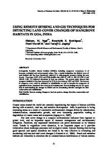
(4,5). Another example is the GLASNOWMAP IS (GLAcier and SNOW MAPping Information Service) that constitutes a new approach for the monitoring of glacier and snow cover changes in the Alpine regions. In this context, remote sensing is a convenient tool for mapping ice expansion and may be seriously regarded as adequate alternative over wide areas, where few direct measurements are available. In a period of 10 years a lot of studies in glacier monitoring from space have been published (6,7). Although changes in glacier thickness cannot be measured directly from optical satellite data, it is possible to perform a classification technique of image time series giving in an indirect way some parameters (i.e. the snow line position on the image) that set a correlation with the Equilibrium Line Altitude (ELA) and the annual net surface balance (8,9). Furthermore, integrating the results of remote sensing image classification with other series of data in raster and vector form in a geo-database, it is possible to extrapolate other meaningful parameters (i.e. Accumulation Area Ratio (AAR)) to evaluate the glacier dynamism (10,11). THE DEVELOPMENT OF A METHODOLOGY IN OPEN SOURCE ENVIRONMENT Data Collection Three groups of studied glaciers (Adamello, Ortles-Cevedale, Bernina) are located in the Italian Alps zone, between latitude of 46-57°N and longitude of 9-11°E, with ice field elevation ranging from 2600 m to 4000 m a.s.l. (Figure 1).

Figure 1: The investigated area. Sub-maps of three Landsat scenes were investigated. They were acquired with the sensors MSS (08/06/1976) (60 m re-sampled), TM (16/08/1992) and ETM+ (13/09/1999) (30 m nominal), downloaded freely from the NASA web site. These data were acquired during the summer months (June-Sept) under cloudless conditions during the end of each hydrological year, mainly in the optical sensor mode (visible to near- and mid-infrared). Such raster information was combined with other types of correlated data: the Lombardia Region Geographical Information System database, the Technical Map at the scale 1:10.000 and the DTM at level 1 with grid spacing of 20 metres of the same Region, the Trento Province DTM in raster grid with 10 metres of spacing. Every performed phase was illustrated by the software ILWIS 3.4 (Integrated Land and Water Information System), developed by the ITC of Enschede and open source from July 2007. It is a Geographic Information System with Image Processing capabilities (http://www.itc.nl/ilwis/).

EARSeL eProceedings 7, 2/2008

122

Data Processing Overview Different image processing techniques were tested for the enhancement and analysis of remote sensing data by means of the software ILWIS 3.4. At first we focused our attention on the georeferencing tool referred to the correction of the geometric distortions which is used to create the relationship between the image and a coordinate system by means of transformation functions and re-sampling techniques. Then the performance of the spectral classification tools related to computer-assisted interpretation of remotely sensed data was underlined. These results were also compared with other meaningful parameters in GIS environment. The different glacier mapping methods presented here can be found in literature (12). In Figure 2 some steps of this analysis are briefly illustrated in a conceptual map.

Figure 2: Data processing conceptual map. The geometric distortion correction Remote sensing data affected by geometric distortions due to sensor geometry, scanner and platform instabilities, earth rotation, earth curvature, etc., can be corrected by referencing the images to existing maps. Furthermore in order to integrate these data with others in a GIS, not only a geometrical correction is necessary, but also a re-sampling adaptation to the same resolution and projections of every other data set. To establish this relationship among the Landsat images and the Gauss-Boaga Italian cartographic datum we performed the georeference tie-points tool in ILWIS applying an affine transformation (Figure 3) by selecting 10 tie-points localised in the vector Technical Map of the Lombardia Region and in the visual RGB synthesis of the most suitable band composition (Figure 4). The sigma gave a measure for the overall accountability of the active tiepoints underlining an accuracy below the pixel (Table 1).

Figure 3: The georeference tie-points.

EARSeL eProceedings 7, 2/2008

123

Figure 4: Georeference processing of the ETM+ image in ILWIS. Table 1: The result of the georeferencing process. sensor MSS (1976) TM (1992) ETM+ (1999)

accuracy (pixel) 0,405 0,634 0,534

A gap was found while performing the georeference task in ILWIS: the use of the DTM was not implemented in the georeferencing tool, which, on the contrary, was very useful in correcting the distortions caused by the altitude in mountainous zones. However, this disadvantage could be overcome by implementing a suitable new procedure performing an orthoimage based on the DTM, according to the open source philosophy. Classification domain and multi band data processing (NDSI and segmentation of ratio images) Remote sensor images consist of many layers or bands created by collecting energy in specific wavelengths of the electro-magnetic spectrum. Such information can be analyzed to extract land use classes. The list of the classes that can occur in the mapping process is called “domain” in ILWIS. The classification process needs, first of all, to create a domain for the TM and ETM+ images satisfying the characteristics of the glaciers and consisting of few detailed land cover classes, as documented in literature (13): Rock, Vegetation, Water bodies, Null, Ablation Glacier Area, Accumulation Glacier Area. The two latter ones indicate the regions where the mass balance between the winter snowy precipitation and the summer withdrawal, evaporation, sublimation is positive and negative, respectively. On the contrary, the poor spectral information of the MSS image reduce the classification domain at the parent classes: Rock, Vegetation, Water bodies, Glacier. To improve the performance of multi-spectral image classification the original image bands were not used directly, but a combination of them (pseudo-images) which enhance and extract features not always clearly detectable in a single band. A mathematical combination of satellite channels, indicating the presence of snow and glacier, is the Normalized Difference Snow Index (NDSI). In this case the NDSI index was obtained using the relationship between the ETM2 and ETM5 channels for the ETM+ sensor, while for the MSS sensor the relationship that involved the channels MSS4 and MSS2 was used.

EARSeL eProceedings 7, 2/2008

124

The NDSI index allows the glacier to be distinguished correctly from every other element with similar brightness as the clouds, the illuminated soil, the vegetation and the rocks (Figure 5) (14,15). This index allows one, though not in an optimal way, to distinguish the accumulation and ablation zones.

Figure 5: The single bands ETM+2, ETM+5 and the NDSI index. Another important process is the segmentation of ratio images. The ratio images are often useful for discriminating differences in spectral variations in a scene that is masked by brightness dissimilarity. Different spectral ratio images are possible; the utility of them depends on the particular reflectance characteristics of the involved features and of the required application. In literature some examples of ratio images with TM3/TM5 and TM4/TM5 channels after threshold are documented, useful to obtain a glacier mask (16,17) or depict different ice and snow faces within a glacier (18). In our application, too, the TM and ETM+ 4/5 ratio images made it possible to distinguish the glacier from the surrounding areas and to make an easy distinction between the accumulation and ablation zones (19). The low reflectivity of snow and glacier ice in the middle infrared part of the spectrum allows a glacier classification from the segmented ETM+4/ETM+5 ratio image (Figure 6) based on specific radiometric values (Table 2).

Figure 6: Segmentation of the ETM+4/ETM+5 ratio image.

EARSeL eProceedings 7, 2/2008

125

Table 2: The threshold value to classify the specific area of interest. Area classified (ETM+) out glacier ablation area accumulation area

Radiometric range 1< >2 4< >10 10< >20

In this map the value range, related to the other classes in respect to the glacier (rocks, vegetation, water bodies, clouds), is restricted. For this reason, the assignment of the sample sets with standard deviation different from zero was very difficult, because this is a necessary characteristic to process the classification algorithm correctly. For this gap this ratio image was not inserted in the main list of the pseudo-images for the classification, but it was used only as reference for a correct identification of the sample sets in the training step. The relationship among channels 4 and 2 was calculated for the MSS sensor. Principal Component Analysis (PCA) Principal Component Analysis (PCA) furnishes a good data compression of image bands into fewer new layers not correlated to each other, with a significant reduction in terms of numerical calculation during the classification process. Applying this type of analysis one obtained other pseudo-images to add to the classification process. The use of these new images was correct because the distance between the pixels (generic criterion of every type of pixel based classification algorithm) resulted unchanged in comparison to the original image in the multi-spectral space. Only four pseudo-images were produced justifying such choice with the fact that the greatest part of the information is contained in the first two or three components (Figure 7). In the TM and ETM+ images the PC1 is a good lighted representation of the natural object, the PC2 allows the glacier coverage to be distinguished from the other elements, as the PC3 which is suitable for separating the accumulation from the ablation zone. On the contrary the last PC4 is useless because it has scarce information. Besides, the association of the three PC images to the RGB colours makes it possible to produce a more informative representation in comparison to each of the other RGB syntheses performed on the original bands. For the MSS sensor only the first component resulted usable.

Figure 7: Principal Component Analysis of the TM sensor data (PC1, PC2, PC3, PC4). Gaussian Maximum Likelihood classification processing The best results were achieved by a supervised Gaussian Maximum Likelihood classification applied to different combinations of pseudo-images in respect to different sensors: TM4/TM5 and ETM+4/ETM+5 and MSS4/MSS2 ratio images, the Natural Difference Snow Index, the PC1-4 carried out from TM and ETM+ images and only the PC1 for the MSS image (20). The algorithm assumes that the feature vectors of each class are (statistically) distributed according to a “multivariate normal probability density function”. The training samples were used to estimate the parameters of the distributions. Such procedure was performed nine times: for every glacier group (Adamello, Bernina, Ortles-Cevedale) and for every multi temporal group of three satellite images

EARSeL eProceedings 7, 2/2008

126

(MSS 1976, TM 1992, ETM+ 1999). Figure 8 puts in evidence the change of land cover between the MSS, TM and ETM+ classification on the Adamello glacier region. It should be noted that the classification derived from the image acquired by the MSS sensor allowed us to determine only information on the dimension of the glacier without further distinctions of the coverage. The segmentation features of the objects are influenced by a large amount of factors, such as atmospheric conditions, sun angle (as function of latitude, time of day, date and terrain relief), soil types, soil humidity, growing stage of the vegetation, wind (affecting orientation of leafs), etc. One could take all these influences into account if one used a vast amount of other additional data (DEM, soil maps, etc.) and performed an “object based” classification method. In this research it is pointed out that the use of the pseudo-images allows to overcome a lot of these problems such as the processing of the shade zones depending on land morphology or the clouds. In fact it is observed that the classification of the TM and ETM+ images using only the principal components matched the assignment of the shade areas very well but underestimated the surface of the glacier. On the contrary a more accurate classification could be derived adding the NDSI images and the ratio images based on the relationships 4/5. The remaining critical areas were the marginal ones to the water bodies.

Figure 8: Adamello MSS-1976, TM-1992, ETM+ 1999 supervised classification. Analysing the histogram of the thematic maps one obtained some numerical information about the coverage (Figure 9) which was very useful in calculating some parameters presented in the next paragraph.

Figure 9: Histogram derived by Adamello ETM+1999 classification.

EARSeL eProceedings 7, 2/2008

127

Since data from field measurements were not available, it was only possible to test the classification accuracy using the false colour composite image (combining the 5, 4 and 3 channels as red, green and blue respectively) and superimposing the segmentation of the glacier area (Figure 10).

Figure 10: RGB synthesis with superimposed ablation (red) and accumulation (yellow) segmentation. ANALYSING THE RESULTS In this section the principal results are summarised by using corresponding methods applied in the GIS combining additional information of different thematic maps coming from the DTM (hill-shading map, altitude map, slope map, aspect map) with land cover classifications, accumulation and ablation vector layers. This underlines the fact that each data was very useful in realising a rigorous monitoring of the condition of the glaciers. The developed GIS analysis in ILWIS gave some glaciological parameters. Obviously the single values of the parameters were not significant in respect to the amount of their variation in the period of observation and the comparison with the threshold based on the literature. The Equilibrium Line Altitude (ELA) represents the “virtual” line of separation between the accumulation of snow and ablation. It is controlled by climatic processes and on this line the balance of mass is in equilibrium (21). So, a rising ELA signifies a glacier in phase of withdrawal, while a lowering implicates a glacier in phase of expansion. In the present case the altitude of ELA has been drawn out from the combination of the DTM with the vector data extracted from the classified images (Figure 11). A raising of the ELA was observed for every glacier (1992-1999) (Table 3). This is much more evident in the Adamello area (Figure 12).

EARSeL eProceedings 7, 2/2008

128

Figure 11: Feature extraction from Cevedale classified images to analyse the ELA parameter. Table 3: The ELA parameters. Glacier Adamello Bernina Ortles-Cevedale

ELA parameters 1992 3000 m 3050 m 3200 m

ELA parameters 1999 3200 m 3300 m 3350 m

Differences 200 m 250 m 150 m

Figure 12: ELA differences related to the Adamello glacier in the period 1992-1999. Another useful parameter to evaluate the surface balance is the Accumulation Area Ratio (AAR). This method is based on the assumption that the accumulation area of the glacier (i.e. the area above the ELA) covers some fixed proportion of the total glacier area. It is calculated as the relationship between the area of accumulation and the total surface extension of the glacier (22,23). The accumulation area of each glacier varies from year to year, depending upon the snow-line at

EARSeL eProceedings 7, 2/2008

129

the end of the ablation season. Also in this case both these elements can be estimated using remote sensing techniques when no field data are available (24,25). Under static conditions the value of AAR is constant, and for middle latitude it is generally in a range of 0.5-0.8 (26). The AAR parameters referred to the three glaciers in a period of observation were very different, but they were so, too, for each glacier in different time series (Table 4). Some possible causes could be the climatic variations or the deposit material coverage. Table 4: The AAR parameters. Glacier Adamello Bernina Ortles-Cevedale

AAR parameters 1992 1999 0,40 0,11 0,31 0,15 0,27 0,19

Figure 13 shows the AAR values referred to the studied areas below the threshold of 0.6. In Table 5 the results for every glacier in the different acquisition periods are summarised. The results confirm the condition of non-equilibrium of the three glaciers.

Figure 13: AAR parameters compared with the threshold value. Table 5: Ablation, accumulation and total surface extension values for each glacier in time series.

Glacier Adamello

Bernina

Ortles-Cevedale

Ablation Accumulation Total surface extension Ablation Accumulation Total surface extension Ablation Accumulation Total surface extension

08/06/1976 MSS sensor (km2) 91.40 222.25 241.90

16/08/1992 TM sensor (km2) 22.87 15.33 38.20 67.13 29.68 96.81 53.30 19.87 73.16

13/09/1999 ETM+ sensor (km2) 29.05 3.66 32.71 63.88 11.00 74.88 50.94 11.82 62.76

EARSeL eProceedings 7, 2/2008

130

The evaluation of the accumulation and ablation values indicated a surface variation of 70% in the period 1976-1999 for each glacier area. This shows a fast and dramatic withdrawal, in line with the global situation (Figure 14).

Surface (km2)

Figure 14: General situation of the glacier surface withdrawal. DISCUSSION Summarising the analysis on the geo database related to the three groups of glaciers Adamello, Bernina and Ortles-Cevedale it must be stated that every obtained parameter evidences similar conditions of non-equilibrium: reduction of the total surface, raising of the equilibrium line and reduction of the AAR. On the other hand, it must be remembered that due to the lack of available data on the thickness of the glaciers only an evaluation of the areas and not of the volumes was possible. To derive some information by the mass balance, useful for evaluating the water resources for the future, it is necessary to know more about glacier attributes, such as the measurements of the thickness of the glacier by surveying campaigns. In any case, to evaluate the condition of the glacier in an annual period the data produced in this research are sufficient. Furthermore, a trend is not proposed because the analysed data were insufficient to make a future forecast. In fact, only three images in 23 years of temporal displacement were analysed, acquired during different summer periods and with different climatic situations. This is not sufficient to make the procedure standard. To overcome this problem constant monitoring is necessary to acquire images in the same period every year. Other remarks are related to the integrated GIS – remote sensing analysis by the ILWIS 3.4 open source environment which reveals the potentiality of these tools (geo-reference, pre-processing of the images, algebra of bands, classification, data analysis, 3D modelling, and layout presentation). The open source software allows a free use and the successive implementation of the presently non- available functions. The ILWIS software is not time consuming during data processing even using a high massive structure of data. It is also a rather intuitive software. In conclusion it can be underlined that the method has the following advantages: simplicity, low cost and reliability. Finally, it had been feasible to collect and demonstrate the main results in the three layouts to give a good visual representation of the data. CONCLUSIONS More refined classification methods, principal components analyses and image rationing can produce a classification which is supported by a rigorous accuracy assessment and can facilitate the production of accurate maps of glacier extention useful for glacier inventory, for change detection studies and also for analysing the influence of climate change and global warming. The acquired location and the extent of each glacier derived by remote sensing techniques can update the database, adding information about the accumulation and ablation areas from which the accumulation

EARSeL eProceedings 7, 2/2008

131

area ratio (AAR) can be derived. Furthermore, the integration of the digital elevation model with the dataset could facilitate the derivation of some other important glacier inventory attributes. Finally, the maintenance of the glacier inventory within a GIS environment allows some queries and reports to be made for every glacier region reducing the need to compile the extensive tabular reports which have characterised past glacier inventories. ACKNOWLEDGEMENTS The GIS dataset was supplied by the Lombardia Region for research purposes. REFERENCES 1

Church J A, J M Gregory et al., 2001. Chapter 11: Changes in Sea Level http://www.grida.no/CLIMATE/IPCC_TAR/WG1/pdf/TAR-11.PDF In: Climate Change 2001: The Scientific Basis, edited by J T Houghton et al. (Cambridge University Press) 639-693 http://www.grida.no/CLIMATE/IPCC_TAR/WG1/index.htm (last date accessed: 19 Sept 2008)

2

Schär C, P L Vidale, D Lüthi, C Frei, C Häberli, M Liniger & C Appenzeller, 2004. The role of increasing temperature variability in European summer heat waves. Nature, 427: 332-336

3

Braun L N, M Weber & M Schultz, 2000. Consequences of climate change for runoff from Alpine regions. Annals of Glaciology, 31: 19-25

4

Kargel J S, H H Kieffer, B Raup, D MacKinnon, K Mullins, the GLIMS consortium, 2000. First results from GLIMS (Global Land Ice Measurements from Space). International Geoscience and Remote Sensing Symposium 2000, Proceedings (IGARSS 2000) (Honolulu, Hawaii) 7: 24-28

5

Raup B H, A Kääb, J S Kargel, M P Bishop, G Hamilton, E Lee, F Paul, F Rau, D Soltesz, S J S Khalsa, M Beedle & C Helm, 2007. Remote sensing and GIS technology in the Global Land Ice Measurements from Space (GLIMS) Project. Computers and Geosciences, 33: 104-125

6

Bindschadler R, J Dowdeswell, D Hall & J G Winther, 2001. Glaciological applications with Landsat-7 imagery : early assessments. Remote Sensing of Environment, 78: 163-179

7

Williams Jr R S, J G Ferrigno, et al., 2007. Introduction (volume A) to series, Satellite Image Atlas of Glaciers of the World, U.S. Geological Survey Professional Paper1386-A

8

Paul F, 2002. Combined technologies allow rapid analysis of glacier changes. EOS Transactions American Geophysical Union, 83(23): 253-261

9

Paul F, A Kääb & W Haeberl, 2007. Recent glacier changes in the Alps observed by satellite: Consequences for future monitoring strategies. Global and Planetary Change, 56/1-2: 111-122

10 König M, J G Winther & E Isaksson, 2001. Measuring snow and glacier ice properties from satellite. Reviews of Geophysics, 39(1):1-27 11 Kargel J S M J Abrams, M P Bishop, A Bush, G Hamilton, H Jiskoot, A Kääb, H H Kieffer, E M Lee, F Paul, F Rau, B Raup, J F Shroder, D Soltesz, D Stainforth, L Stearns & R Wessels, 2005. Multispectral imaging contributions to global land ice measurements from space. Remote Sensing of Environment, 99(1-2): 187-219 12 Paul F, 2000. Evaluation of different methods for glacier mapping using Landsat TM. EARSeL eProceedings, 1: 239-245 http://www.eproceedings.org/static/vol01_1/01_1_paul1.pdf (last date accessed: 01 Oct 2008) 13 Rampini A, P A Brivio, F Rota Nodari & E Binaghi, 2002. Mapping Alpine Glaciers Changes from Space. In: Geoscience and Remote Sensing Symposium, 2002. IGARSS '02. 2002 IEEE International: 2199-2201

EARSeL eProceedings 7, 2/2008

132

14 Hall D K, J P Ormsby, R A Bindschadler & H Siddalingaiah, 1987. Characterization of snow and ice reflectance zones on glaciers using Landsat TM data. Annals of Glaciology, 9, 104108 15 Dozier J, 1989. Spectral signature of Alpine snow cover from the Landsat Thematic Mapper. Remote Sensing of Environment, 28: 9-22 16 Bayr I J, D K Hall & W M Kovalick, 1994. Obervations on glaciers in the eastern Austrian Alps using satellite data. International Journal of Remote Sensing, 15: 1733-1742 17 Paul F, H Machguth & A Kääb, 2005. On the impact of glacier albedo under conditions of extreme glacier melt: the summer of 2003 in the Alps. EARSeL eProceedings, 4(2): 139-149 http://www.eproceedings.org/static/vol04_2/04_2_paul1.html (last date accessed: 01 Oct 2009) 18 Rott H & G Markl, 1989. Improved snow and glacier monitoring by the Landsat Thematic Mapper. In: Proceedings of a Workshop on Landsat Thematic Mapper applications, ESA SP-1102: 3-12 19 Paul F, C Huggel, A Kääb, T Kellenberger & M Maisch, 2002. Comparison of TM-derived glacier areas with higher resolutions data sets. EARSeL eProceedings, 2: 15-21 http://www.eproceedings.org/static/vol02_1/02_1_paul1.pdf (last date accessed: 01 Oct 2009) 20 Gratton D J, P J Howarth & D J Marceau, 1990. Combining DEM parameters with Landsat MSS and TM imagery in a GIS for mountain glacier characterization. IEEE Transactions on Geoscience and Remote Sensing, GE-28: 766-769 21 Torsnes I, N Rye & A Nesje, 1993. Modern and little ice age equilibrium-line altitudes on Outlet Valley Glaciers from Jostedalsbreen, Western Norway: an evaluation of different approaches to their calculation. Arctic, Antarctic and Alpine Research, 25(2): 106-116 22 Meier M F & A Post, 1987. Fast tidewater glaciers. Journal of Geophysical Research, 92(B9): 9051-9058 23 Benn D I & A M D Gemmell, 1997. Calculating equilibrium-line altitudes of former glaciers by the balance ratio method: a new computer spreadsheet. Glacial Geology and Geomorphology, tn01, 7 pp. http://ggg.qub.ac.uk/papers/full/1997/tn011997/tn01.pdf (last date accessed: 08 Oct 2008) 24 Kulkarni A V, 1992. Mass balance of Himalayan glaciers using AAR and ELA methods. Journal of Glaciology, 38: 101-104 25 Kulkarni A V, B P Rathore & A Suja, 2004. Monitoring of glacial mass balance in the Baspa basin using accumulation area ratio method. Current Science, 86(1): 185-190 http://www.ias.ac.in/currsci/jan102004/185.pdf (last date accessed: 01 Oct 2009) 26 Mercer J H, 1961. The response of fjord glaciers to changes in the firn limit. Journal of Glaciology, 3(29): 850-858