Global and Local Spatial Autocorrelation in

Global and Local Spatial Autocorrelation in Predictive Clustering Trees Daniela Stojanova1 , Michelangelo Ceci2 , Annalisa Appice2 , Donato Malerba2 , and Saˇso Dˇzeroski1 1

2

Joˇzef Stefan Institute, Department of Knowledge Technologies, Ljubljana, Slovenia Dipartimento di Informatica, Universit` a degli Studi di Bari, Bari, Italy {daniela.stojanova,saso.dzeroski}@ijs.si, {ceci,appice,malerba}@di.uniba.it

Abstract. Spatial autocorrelation is the correlation among data values, strictly due to the relative location proximity of the objects that the data refer to. This statistical property clearly indicates a violation of the assumption of observation independence - a pre-condition assumed by most of the data mining and statistical models. Inappropriate treatment of data with spatial dependencies could obfuscate important insights when spatial autocorrelation is ignored. In this paper, we propose a data mining method that explicitly considers autocorrelation when building the models. The method is based on the concept of predictive clustering trees (PCTs). The proposed approach combines the possibility of capturing both global and local effects and dealing with positive spatial autocorrelation. The discovered models adapt to local properties of the data, providing at the same time spatially smoothed predictions. Results show the effectiveness of the proposed solution.

1

Introduction

Spatial autocorrelation is a property of random variables taking values, at pairs of locations a certain distance apart, that are more similar (positive autocorrelation) or less similar (negative autocorrelation) than expected for pairs of observations at randomly selected locations [14]. Spatial positive (negative) autocorrelation occurs when the values of a given property are highly uniform (different) among similar spatial objects in the neighborhood. In geography, spatial autocorrelation is justified by Tobler’s [24] first law, according to which “everything is related to everything else, but near things are more related than distant things”. By picturing the spatial variation of some observed variables in a map, we may observe regions where the distribution of values is smoothly continuous. Most statistical models are based on the assumption that the values of observations in each sample are independent of one another, but spatial autocorrelation clearly indicates a violation of this assumption. As observed in LeSage and Pace [15], “anyone seriously interested in prediction when the sample data exhibit spatial dependence should consider a spatial model”, since this can take T. Elomaa, J. Hollm´ en, and H. Mannila (Eds.): DS 2011, LNCS 6926, pp. 307–322, 2011. c Springer-Verlag Berlin Heidelberg 2011 

308

D. Stojanova et al.

into account different forms of spatial autocorrelation. In addition to predictive data mining tasks, this consideration can also be applied to descriptive tasks, such as spatial clustering. In general, the analysis of spatial autocorrelation is crucial and can be fundamental for building a spatial component into (statistical) models for spatial data. The inappropriate treatment of sample data with spatial dependence could obfuscate important insights and the observed patterns may even be inverted when spatial autocorrelation is ignored [13]. Although spatial autocorrelation has been taken into account when analyzing spatial data both for predictive purposes and descriptive tasks [5] [18] [21] [15], less attention has been given in the literature to data mining methods for spatial data that combine predictive and descriptive modeling and take spatial autocorrelation into account. The task we focus on in this paper is that of predictive clustering [2]. Predictive clustering combines elements from both prediction and clustering. As in clustering, clusters of examples that are similar to each other are identified, but a predictive model is associated to each cluster. The predictive model assigns new instances to clusters based on their description and provides a prediction for the target property. The benefit of using predictive clustering methods, as in conceptual clustering [20], is that, besides the clusters themselves, they also provide symbolic descriptions of the constructed clusters. However, differently from conceptual clustering, predictive clustering is a form of supervised learning. Predictive clustering trees (PCTs) are tree structured models that generalize decision trees. Their properties are that i) they can be used to predict many or all attributes of an example at once, ii) they can be applied to a wide range of prediction tasks (classification and regression) and iii) they can work with examples represented by means of a complex representation [7]. This is achieved by plugging in a suitable distance metric for the task at hand. In the context of this paper, PCTs can be easily extended to spatial data in order to take spatial autocorrelation into account. Motivated by the complexity of spatial data and its characteristics, in this paper, we propose a predictive clustering approach that learns spatial models in the form of PCTs. The distinctive characteristic of the proposed approach in comparison to classical PCTs is that it explicitly takes positive spatial autocorrelation into account. The method extends the predictive clustering framework implemented in the CLUS system [2]1 and, concentrating on the regression task, we modify the search strategy in order to take into account the complex structure of spatial data and, in particular, the spatial arrangement of objects over space. In this way, it is possible to consider different effects of the autocorrelation phenomenon at different levels of the tree (global vs. local effect of autocorrelation). At the same time, the tree structure allows us to deal with the so-called “ecological fallacy” problem [22] according to which individual sub-regions do not have the same data distribution of the entire region. Our goal is to build spatially-aware PCTs that use the spatial information as background knowledge and can be used to obtain spatially coherent predictions. The main assumption is that if there is a high autocorrelation between the 1

The CLUS system is available at http://www.cs.kuleuven.be/∼dtai/clus.

Global and Local Spatial Autocorrelation in Predictive Clustering Trees

309

examples in the dataset, not only the examples have similar target values but also they are in the same spatial neighborhood. This provides an unique opportunity to increase the accuracy of the predictive models without performing spatial splits that can lead to loosing generality of the induced models. The paper is organized as follows. The next section reports relevant related work. Section 3 describes the proposed approach. Section 4 describes the datasets, experimental setup and reports relevant results. Finally, in Section 5 some conclusions are drawn and some future work outlined.

2

Related Work

The motivation for this work comes from research reported in the literature for spatial autocorrelation and predictive clustering. In the following subsections, we report related work from both research lines. 2.1

Spatial Autocorrelation

The effect of spatial autocorrelation has been examined in several data mining studies. One of the first works that recognized the importance of considering spatial autocorrelation in spatial data mining, presented by Huang et al. [11], proposes and empirically validates methods based on logistic regression and Bayesian classification that explicitly take the spatial dimension into account. In a theoretical study, LeSage and Pace [15] stress that the presence of spatial dependence requires an appropriate treatment of spatial correlation effects. They show how the inclusion of autocorrelation of the dependent variable provides an improvement in fit, as well as dramatic differences in inferences drawn concerning the significance and impact of explanatory variables. Several spatial data mining approaches have discussed and considered autocorrelation in solving different data mining tasks. For example, spatial autocorrelation has been exploited by Zhang et al. [25], to efficiently process similarity based range queries and joins that take correlation into account when retrieving spatial time series. Scrucca [23] proposed a clustering procedure for identifying spatial clusters, based on the contiguity structure of objects and their attribute information. The procedure uses a K-means algorithm that incorporates the spatial structure of the data through the use of measures of spatial autocorrelation. In the context of predictive data mining, spatial autocorrelation has been considered for classification tasks. Spatial decision trees proposed by Li and Claramunt [16] use “spatial entropy” which captures autocorrelation to adapt classification trees for handling geographical data. Bel et al. ([1]) modify Breiman’s classification trees ([3]) to take into account the irregularity of sampling by weighting the data according to their spatial pattern (using Voronoi tessellations, a regular grid, and kriging). For regression, a standard way to take into account spatial autocorrelation in spatial statistics is Geographically Weighted Regression (GWR) [9]. GWR extends the traditional regression framework so that all parameters are estimated within a local context. In this way, GWR takes

310

D. Stojanova et al.

advantage of positive autocorrelation between neighboring points in space and provides valuable information on the nature of the processes being investigated. In general, incorporating spatial autocorrelation into regression can be a serious issue because the presence of spatial autocorrelation may alter the observed patterns as well as the error probabilities of the linear models [13]. A recent trend to avoid to modify classical data mining algorithms when dealing with autocorrelation is to resort to the relational data mining setting. For example, Ceci and Appice [5] propose a spatial associative classifier that learns, in the same learning phase, both association rules and a classification model (on the basis of the extracted rules) whereas Malerba et al. [17] present a multi-relational clustering algorithm (CORSO) that expresses relationships by resorting to the First Order Logic representation formalism and uses learning in the Normal ILP setting. In this way, it can take into account the autocorrelation embedded in the discrete spatial structure. In the clustering phase, the similarity of multi-relational descriptions is used in order to identify examples that are in the neighborhood. For regression, Malerba et al. [18] present a relational regression method that captures both global and local spatial effects of the explanatory attributes, while building a regression model tightly integrated with a spatial database. However, when resorting to relational data mining, it is possible that the presence of autocorrelation in spatial phenomena can bias feature selection [12]. In particular, the distribution of scores for features formed from related objects with concentrated linkage (i.e., high concentration of objects linked to a common neighbor) has a surprisingly large variance when the class attribute has high autocorrelation. This large variance causes feature selection algorithms to be biased in favor of these features, even when they are not related to the class attribute, that is, they are randomly generated. In this case, conventional hypothesis tests, such as the χ2 -test for independence, which evaluate statistically significant differences between proportions for two or more groups in a dataset, fail to discard uninformative features. 2.2

Building Predictive Clustering Trees

The task of learning predictive clustering trees can be formalized in this way: Given • a descriptive space X = X1 , X2 , . . . Xm , • a target space Y , • a set T of examples (xi , yi ) with xi ∈ X and yi ∈ Y Find • a set of hierarchically organized clusters defined according to X × Y , • a predictive piecewise function f : X → Y , defined according to the hierarchically organized clusters. The clusters to be found are defined on the basis of examples in T and represented according to both the descriptive space and the target space X × Y . This is different from what is commonly done in predictive modeling and classical clustering, where only one of the spaces is considered.

Global and Local Spatial Autocorrelation in Predictive Clustering Trees

311

Note that this general formulation of the problem can take into account different aspects: a) multiple target attributes can be considered at the same time; b) the distance function used in the clustering phase can consider the (possible) complex nature of the data c) this formulation is valid both for classification and regression problems (it depends on the nature of Y and on how the function f (·) is built). In PCTs [2], a decision tree is viewed as a hierarchy of clusters: the top-node corresponds to one cluster containing all data, which is recursively partitioned into smaller clusters while moving down the tree. The construction of PCTs is not very different from that of standard decision tree learners: at each internal node t, a test has to be defined according to a given evaluation function. The main difference is that PCTs select the best test by maximizing the (inter-cluster)  k| variance reduction, defined as ΔX (E, P) = Var (E)− Ek ∈P |E |E| Var(Ek ), where E represent the examples in t and P defines the partition2 {E1 , E2 } of E. If the variance V ar(·) and the predictive function f (·) are considered as parameters, instantiated for the specific learning task at hand, it is possible to easily adapt PCTs to different domains and different tasks. To construct a regression tree, for example, the variance function returns the variance of the given instances’ target values, and the predictive function is the average of target values in a cluster. Indeed, by appropriately defining the variance and predictive functions, PCTs have been used for clustering ([2]), multi-objective classification and regression ([2]; [6]), and time series data analysis ([7]). In this paper, we propose to extend the problem of constructing PCTs by taking the spatial dimension in form of background knowledge in addition to the descriptive and target spaces, to explicitly consider spatial autocorrelation.

3

Learning Spatial PCTs

In order to formalize the learning task we are referring to, we need to define the spatial dimension of the data with the goal of explicitly taking spatial autocorrelation into account. For this purpose, in addition to the descriptive space X and the target space Y , it is necessary to add information on the spatial structure of the data in order to be able to capture the spatial arrangement of the objects (e.g. the coordinates of the spatial objects involved in the analysis or the pairwise distances between them). Concentrating on the regression task, we have to consider different aspects: i) What attributes should be considered in the tests in the internal nodes of the tree? ii) Which evaluation measure for the tests, taking spatial dimension into account, would lead to the best clustering? iii) What distance measure should be used when taking into account spatial autocorrelation? 2

Note that we will consider binary decision trees, hence the partitions are {E1 , E2 } rather than the general case of {E1 , E2 , ..., Em }.

312

D. Stojanova et al.

Concerning i), a na¨ıve solution would consider both the descriptive and the spatial attributes as candidates in a test associated to the split. However, this solution, would lead to models that would be difficult to apply in the same domain, but in different spatial contexts. For this reason, following Ester et al. [8], we do not consider spatial information in the candidate tests. This limitation of the search space allows us to have more general models, at the price of possible loss in predictive power of the induced models. Concerning ii), CLUS uses the variance reduction as an evaluation measure. However, in order to take the spatial autocorrelation into account when partitioning the descriptive space, a different measure is necessary. In spatial analysis, several spatial autocorrelation statistics have been defined. The most common ones are Global Moran’s I and Global Geary’s C [14]. These require a spatial weights matrix that reflects the intensity of the spatial relationship between observations in a neighborhood. Formula (1) defines the Global Moran’s I as   N i j wij (Xi − X)(Xj − X) IX = (1)  W i (Xi − X)2 where N is the number of spatial objects (examples) indexed by i and j; Xi and Xj are the values of the variable X for the objects oi and oj , respectively; X is  the variable of interest; X is the overall mean of X; and W = i,j wij is the sum of spatial weights wij , i, j = 1, . . . , N . Values that are more positive than expected indicate positive autocorrelation, while more negative values indicate negative autocorrelation. Values generally range from -1 to +1 and 0 indicates a random distribution of the data. Global Geary’s C is defined as   (N − 1) i j wij (Xi − Xj ) (2) CX =  2W i (Xi − X)2 Its values typically range from 0 (positive autocorrelation) to 2 (negative autocorrelation) and 1 indicates a random distribution of the data. While both statistics reflect the spatial dependence of values, they do not provide identical information: C emphasizes the differences in values between pairs of observations, while I emphasizes the covariance between the pairs. This means that Moran’s I is smoother, whereas Geary’s C is more sensitive to differences in small neighborhoods. Concerning iii), the weights wij used in equations (1) and (2) are defined as the inverse of a spatial distance measure. The essential idea is that the observations near to a particular object have more influence in the estimation of its value than do objects farther away. One obvious choice is: 2

2

wij = e(−dij /b

)

(3)

where b is referred to as the bandwidth and dij is the Euclidean spatial distance between objects oi and oj . If oi and oj are placed at the same location, wij = 1. The weighting of other data will decrease according to a Gaussian curve, as the distance between oi and oj increases. If oi and oj are far away from each

Global and Local Spatial Autocorrelation in Predictive Clustering Trees

313

Algorithm 1. Top-down induction of SpatialPCTs 1: procedure SpatialPCT(E) returns tree 2: if stop(E) then 3: return leaf(Prototype(E)) 4: else 5: (v ∗ , h∗ , P ∗ ) = (null, 0, ∅) 6: for each possible test v do 7: P = partition induced by v on E (1 − α)  α  ΔT (E, P) + ST (P, E) 8: h= |T | T ∈Y |T | T ∈Y

9: if (h > h∗ ) then 10: (v ∗ , h∗ , P ∗ ) = (v, h, P) 11: end if 12: end for 13: for each Ek ∈ P ∗ do 14: tree k = SpatialPCT(Ek ) 15: end for  16: return node(v ∗ , k {tree k }) 17: end if

other, wij will tend to zero, excluding these observations from the estimation of parameters for oi . We refer to this weighting function as “Gaussian”. In addition, we use a weighting function linearly dependent on the inverse Euclidean distance (4) and a modified Gaussian kernel density function (5): wij = (1 − dij /b)

(4)

wij = (1 − d2ij /b2 )

(5)

which we refer to as “Euclidean” and “Modified”, respectively. Whatever weighting function is selected, the estimated parameter surfaces will be, in part, functions of the definition of that weighting function. 3.1

The Algorithm

We can now proceed to describe the top-down induction algorithm for building Spatial PCTs (Algorithm 1). It is a recursive method which takes as input a set of training instances E and partitions the descriptive space until a stopping criterion is satisfied (Algorithm 1, line 2). The main loop (Algorithm 1, lines 6-11) searches for the best attribute-value test v∗ that can be associated to a node t. It associates the best test v ∗ with the internal node t and calls itself recursively to construct a subtree for each subset (cluster) in the partition P ∗ induced by v ∗ on the training instances. As discussed above concerning i), splits are derived only from the descriptive attributes. Possible tests are of the form X ≤ β for continuous attributes, and X ∈ {xi1 , xi2 , . . . , xie } (where {xi1 , xi2 , . . . , xie } is a subset of the domain DX of X) for discrete attributes. For continuous attributes, possible values of β are

314

D. Stojanova et al.

found by sorting the distinct values of X in the training set associated with t, then considering a threshold between each pair of adjacent values. Therefore, if the cases in t have k distinct values for X, at most k − 1 thresholds are considered. When selecting a subset of values for a discrete attribute, we rely on a non-optimal greedy strategy [19]. It starts with an empty set Lef tt =  and a full set Rightt = DX , where DX is the domain of X. It moves one element from Rightt to Lef tt such that the move results in increased variance reduction. This differs from the classical solution [3], where some ordering on the possible values of DX is defined apriori, according to the data distribution. However, the classical solution cannot deal with multi-objective predictive tasks as we do. The algorithm evaluates the best split according to the formula reported in Algorithm 1, line 8. This formula is a linear combination of the variance reduction and the statistic SX (P, E). If autocorrelation holds, examples with high spatial autocorrelation (close to each other in space) will fall in the same cluster and will have similar values of the response variables. In this way, we are able to keep together spatially close examples without forcing spatial splits (which can result in loosing generality of the induced models). According to the above discussion of ii), SX (P, E) can be defined in terms of both Moran’s I and Geary’s C. However, since IX and CX range in different intervals, it is necessary to appropriately scale them. We decided to scale both in the interval [0,2], where 2 means high positive autocorrelation and 0 means high negative autocorrelation. For example, for Moran’s I, SX (P, E) is:  |Ek | · I SX (P, E) = 1/|E| · X (Ek ) Ek ∈P

where I X (Ek ) is the scaled Moran’s I computed on Ek . Moreover, in order to guarantee a fair combination of the variance reduction and the statistic SX (P, E), we also need to scale the variance reduction in the interval [0,2]. For that purpose, we use a common scaling function: Δ(E, P) = 2

Δ(E, P) − Δmin Δmax − Δmin

(6)

where Δmax and Δmin are the maximum and the minimum values of Δ(E, P) for a particular split. √ The search stops when the number of the examples in a leaf is less than N , which is considered a good locality threshold that does not permit to lose too much in accuracy also for rule based classifiers [10]. When the stopping criterion is satisfied, the algorithm creates a leaf and labels it with a predictive function (in this case, the average) defined for the instances falling in that leaf. When predicting multiple variables, the predictive function is an aggregation function (in this case, the average) over tuples of target values. Each target variable contributes equally to the overall h value.

Global and Local Spatial Autocorrelation in Predictive Clustering Trees

3.2

315

Estimating the Bandwidth

The choice of the bandwidth (in this study presented as a percentage of the maximum distance between examples and denoted by b in (3)) is perhaps the most critical decision to be taken in the modeling process. This parameter controls the degree of smoothing. A small bandwidth results in very rapid distance decay, whereas a larger value will result in a smoother weighting scheme. At the same time, this parameter influences the level of spatial autocorrelation. The bandwidth may be defined manually or by using some form of adaptive method, such as cross validation and the corrected Akaike Information Criterion (AIC), as used in GWR [9]. In this study, for the bandwidth estimation we minimize the leave-one-out cross validated - Root Mean Square Error (CV-RMSE). Minimization is performed by means of the Golden section search [4] that aims, in this case, at binary recursively partitioning of the bandwidth domain. Parti√ tions are not uniform in width, but maintain the golden ratio γ = 1+2 5 . For each couple of bandwidth values, b1 and b2 (at the first iteration, they are initialized as minimum and maximum bandwidth, respectively), the algorithm identifies a point b3 between them, according to the golden ratio and computes the CVRMSE for that point (RM SEb3 ). The algorithm than identifies the only parabola with a vertical axis that intersects the points {(b1 , RM SEb1 ), (b3 , RM SEb3 ), (b2 , RM SEb2 )}. On the basis of the position of the minimum of this parabola, it decides whether to consider (b1 , b3 ) or (b3 , b2 ) as the next couple of bandwidth values. The search stops when there is no CV-RMSE reduction. In the algorithm, RMSE is computed by fitting a weighted linear model for the left out example. Weights are defined according to (3). 3.3

Time Complexity

The computational complexity of the algorithm depends on the computational complexity of adding a splitting node t to the tree, which in fact depends on the complexity of selecting a splitting test for t. A splitting test can be either continuous or discrete. In the former case, a threshold a has to be selected for a continuous variable. Let N be the number of examples in the training set, then the number of distinct thresholds can be N -1 at worst. They can be determined after sorting the set of distinct values. If m is the number of descriptive variables, the determination of all possible thresholds has a complexity O(m ∗ N ∗ logN ) when an optimal algorithm is used to sort the values. For each of the possible thresholds, the system has to compute the measure used of the evaluation of a single split. This computation has, in principle, timecomplexity O(N 2 ), however, it is not necessary to recompute it at each splitting evaluation since partial sums can be incrementally updated depending on the examples that are moved from the right to the left branch. This optimization makes the complexity of the evaluation of a single split O(N ). This means that the worst case complexity of adding a splitting node on a continuous attribute is O(m∗(N logN +N )), that is O(m∗N logN ). Similarly, for a discrete splitting test, the worst case complexity is O(m ∗ k ∗ N ), where k is the maximum number of

316

D. Stojanova et al.

distinct values of a discrete variable (k ≤ N ). Therefore, finding the best splitting node (either continuous or discrete) has a complexity of O(m ∗ N logN ). For the induction of a complete clustering tree, this complexity, in the worst case, is O(z ∗ m ∗ N logN ), where z is the number of internal nodes in the tree.

4

Empirical Evaluation

In this Section, we present an empirical evaluation of the system SCLUS that implements the method SpatialPCTs presented in Section 3. First, we investigate variations of the method along the dimensions of the different weighting functions and different evaluation measures used in the splitting evaluation, as well as the sensitivity of the algorithm to the value of the bandwidth b and to the value of α. Second, we evaluate the method for automatic determination of the bandwidth, presented in Section 3.2. Third, we compare SCLUS performance on real world datasets to competitive regression and spatial modeling methods. Before we proceed to presenting empirical results, we provide a description of the used datasets and experimental settings. 4.1

Datasets

In this experimental evaluation, we use real world data that includes a spatial component. We consider five datasets. NWE (North-West England) contains census data concerning the North West England area, i.e., the percentage of mortality (target variable) and measures of deprivation level in the ward according to index scores such as the Jarman Underprivileged Area Score, Townsend score, Carstairs score and the Department of the Environments Index, as well as the coordinates of the ward centroid. The datasets SIGMEA MS and SIGMEA MF (MS and MF) [6] are derived from one multi-objective dataset containing measurements of pollen dispersal (crossover) rates from two lines of plants (target variables), that is, the transgenic male-fertile (MF) and the non-transgenic male-sterile (MS) line of oilseed rape. The predictor variables are the cardinal direction and distance of the sampling point from the center of the donor field, the visual angle between the sampling plot and the donor field, and the shortest distance between the plot and the nearest edge of the donor field, as well as the coordinates of the sampling point. We are considering both targets together as well as each target separately. The FOIXA dataset contains measurements of the rate of contamination (target variable) at sampling points located within a conventional field that comes from the surrounding genetically modified (GM) fields within a 400 ha large maize oriented production area in the Foixa region in Spain. The explanatory variables include the number of GM fields, the size of the surrounding GM fields, the ratio of the size of the surrounding GM fields and the size of conventional field, the average distance between conventional and GM fields, as well as the coordinates of the sampling points. The GASD (USA Geographical Analysis Spatial Dataset) [21] contains observations on US county votes cast in the 1980 presidential election. Specifically, it contains the

Global and Local Spatial Autocorrelation in Predictive Clustering Trees

317

Table 1. Dataset descriptions. N – number of examples, Atr. – number of descriptive attributes and Global Moran’s I for different bandwidth values (expressed in percentage of the maximum spatial distance between two examples in the dataset). The automatically estimated bandwidth values are given in brackets. Results of MS and MF with 1% are not available due to the sparsity of the dataset. Dataset

N

NWE MS MF FOIXA GASD

970 817 817 420 3106

Atr. Spatial autocorrelation (Global Moran I) 1% 5% 10% 20% 100% estim.(b) 4 0.19 0.06 0.04 0.02 0.00 0.05 (7.67%) 4 NaN 0.39 0.26 0.17 0.00 0.40 (4.80%) 4 NaN 0.27 0.20 0.14 0.00 0.21 (9.14%) 9 0.15 0.09 0.10 0.07 0.01 0.00 (64.6%) 4 0.59 0.48 0.40 0.28 0.03 0.53 (2.50%)

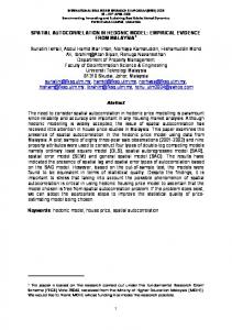
Fig. 1. An example of the effect of the spatial autocorrelation on US presidential votes cast in 1980. Red (blue) denotes high positive (negative) spatial autocorrelation of the votes. The figure shows that voting is indeed driven by some spatial processes.

total number of votes cast per county (target attribute), the population above 18 years of age in each county, the number of owner-occupied housing units, the aggregate income and the coordinates of the county. A description of the datasets is provided in Table 1 where we also report the spatial autocorrelation computed by means of the Global Moran I using different bandwidth values. The level of the spatial autocorrelation very much depends on the dataset and on the bandwidth. The spatial autocorrelation of the GASD dataset is shown in Figure 1. When the autocorrelation is (relatively) high only for the small values of the bandwidth, it is limited to a small neighborhood. This is the case for the NWE and GASD datasets. In contrast, when it is (relatively) high for higher values of the bandwidth, autocorrelation affects larger neighborhoods, as for the other datasets (MS, MF and FOIXA). 4.2

Experimental Setup

The performance of each algorithm on each of the 5 datasets is estimated by means of 10-fold cross validation and evaluated according to the Relative Root Mean Squared Error (RRMSE). RRMSE is defined by formula (7) as the RMSE of the prediction normalized with the RMSE of the default model, i.e., the model that always predicts (for regression) the average value of the target:

318

D. Stojanova et al.

RRM SE =

  j=1,...,N

(f (xj ) − yj )2

 

(y − yj )2

(7)

j=1,...,N

where N is the number of testing examples, yj are the observed target values, f (xj ) the predicted ones and y is the average of the real target variable on the test set. The normalization removes the influence of the range of the target. The predictive performance of the proposed system SCLUS is compared with that of the CLUS algorithm, as well as to a modification of CLUS that considers the coordinates as target variables, along with the actual response variables, for the computation of the evaluation measure (henceforth CLUS*). The latter introduces the spatial dimension into CLUS without modifying the algorithm itself. In this way, the predictive models do not loose their generality and can be applicable for different spatial context in the same domain. Moreover, if there is a strong autocorrelation then it makes sense to try to make splits that yield subsets that are also coherent geographically, since this makes it more likely that the target values will indeed be more similar. Obviously, we do not use coordinates in the evaluation. In addition, SCLUS is compared to other competitive regression algorithms M5’ Regression Trees (RT), M5’ Rules (both implemented in the WEKA framework) and Geographically Weighted Regression (GWR). Only GWR, SCLUS and CLUS* consider the autocorrelation. 4.3

Results and Discussion

Table 2 shows the effect of the weighting function and its contribution within the splitting criterion. The best results in terms of RRMSE for each bandwidth value are given in bold. The analysis of the results reveals that the best results are obtained by combining the Euclidean weighting function with the Moran statistic and the Gaussian weighting function with the Geary statistic. Note that for this comparison we set α = 0, i.e., the algorithm considers only the spatial autocorrelation and ignores the variance reduction. Comparing the results obtained at different bandwidths, we can see that the manual selection of the bandwidth does not lead to a general conclusion for all datasets. The weighting function that is most sensitive to the bandwidth value is the Euclidean distance. In Table 3, we report the RRMSE results for SCLUS using the automatically estimated bandwidth. In most cases, the automatic estimation improves the predictive power of the models obtained with a manual selection of the bandwidth. The selection of the user-defined parameter α is a very important step, influencing the learning process. The simplest solution is to set this parameter to 0 (consider only the spatial statistics) or 1 (consider only the variance reduction for regression, as in the original CLUS algorithm). Any other solution will combine the effects, allowing both criteria to influence the split selection. Table 3 also presents the RRMSE of the proposed algorithm, obtained by varying the parameter α in {0, 0.5, 1}. From the results we can see that the use of α = 0.5 is beneficial in most of the cases which confirms the assumption made in Section 1, especially for datasets (MS, MF and FOIXA) where the effect of the autocorrelation is not limited to small neighborhoods.

Global and Local Spatial Autocorrelation in Predictive Clustering Trees

319

Table 2. Average RRMSE of the SCLUS models learned with different weighting functions, evaluation measures, bandwidth values and α=0.0. The best results for each bandwidth value are given in bold. Dataset NWE Moran MS MF FOIXA GASD NWE Geary MS MF FOIXA GASD

Mod. 0.983 0.753 0.762 0.889 0.877 0.987 0.743 0.665 0.878 0.915

1% Gauss. 0.986 0.753 0.759 0.893 0.881 0.987 0.743 0.665 0.882 0.919

Euc. 0.983 0.753 0.759 0.889 0.872 0.991 0.743 0.665 0.877 0.920

Mod. 0.984 0.695 0.759 0.893 0.875 0.987 0.697 0.777 0.889 0.889

5% Gauss. 0.985 0.761 0.699 0.893 0.875 0.986 0.733 0.703 0.889 0.916

Euc. 0.981 0.699 0.769 0.893 0.877 0.988 0.809 0.759 0.894 0.889

Mod. 0.982 0.791 0.726 0.897 0.868 0.986 0.771 0.766 0.886 0.857

10% Gauss. 0.982 0.707 0.760 0.903 0.866 0.986 0.771 0.766 0.886 0.855

Euc. 0.979 0.765 0.801 0.903 0.882 0.986 0.771 0.766 0.884 0.894

Mod. 0.982 0.747 0.756 0.903 0.875 0.987 0.788 0.766 0.893 0.789

20% Gauss. 0.979 0.765 0.801 0.903 0.880 0.988 0.766 0.766 0.886 0.845

Euc. 0.982 0.774 0.750 0.902 0.875 0.986 0.771 0.766 0.887 0.840

Table 3. Average RRMSE of the SCLUS models learned by using an automatically estimated b, compared to other methods. The best results are given in bold. Dataset

b (%)

NWE MS MF FOIXA GASD Dataset

7.67 4.8 9.14 64.62 2.5 b (%)

NWE 7.67 MS 4.8 MF 9.14 FOIXA 64.62 GASD 2.5

SCLUS (Moran) α=0 α=0.5 Mod. Gauss. Euc. Mod. Gauss. 0.981 0.981 0.994 0.999 0.999 0.845 0.821 0.621 0.849 0.821 0.833 0.833 0.649 0.833 0.833 0.342 0.436 0.545 0.342 0.334 0.880 0.875 0.878 0.851 0.869 SCLUS (Geary) α=0 α=0.5 Mod. Gauss. Euc. Mod. Gauss. 1.000 1.002 1.002 0.999 0.999 0.668 0.883 0.749 0.849 0.821 0.802 0.838 0.833 0.833 0.833 0.671 0.308 0.496 0.342 0.334 0.851 0.858 0.904 0.851 0.869

Euc. 1.023 0.603 0.567 0.242 0.856

Euc. 1.015 0.535 0.638 0.359 0.866

CLUS CLUS* M5’ (α = 1) RT

M5’ GWR Rules

0.988 0.690 0.729 0.892 0.804 CLUS (α = 1)

0.999 0.743 0.761 0.974 0.800 M5’ RT

1.001 0.969 0.700 2.0581 0.665 6.544 0.997 1.051 0.812 1.867 M5’ GWR Rules

0.993 0.999 0.781 0.743 0.787 0.761 0.871 0.974 0.803 0.800

1.001 0.969 0.700 2.0581 0.665 6.544 0.997 1.051 0.812 1.867

0.988 0.690 0.729 0.892 0.804

0.993 0.781 0.787 0.871 0.803 CLUS*

Table 4. Global Moran I of the errors of the obtained models. Best results are in bold. Dataset NWE MS MF FOIXA GASD

SCLUS-Geary α=0 Mod. Gauss. Euc. 0.07 0.00 0.06 0.26 0.29 0.24 0.18 0.21 0.20 0.01 0.01 0.01 0.16 0.14 0.17

SCLUS-Geary α=0.5 Mod. Gauss. Euc. 0.07 0.00 0.07 0.31 0.23 0.26 0.23 0.02 0.17 0.01 0.01 0.01 0.16 0.13 0.17

CLUS CLUS* M5’ (α = 1) RT 0.00 0.00 0.00 0.48 0.32 0.34 0.26 0.13 0.19 0.01 0.00 0.00 0.13 0.37 0.37

M5’ GWR Rules 0.00 0.00 0.26 0.38 0.14 0.19 0.00 0.01 0.37 0.39

In Table 3, we can also compare SCLUS with other competitive methods (CLUS, CLUS*, Regression Trees and Rules, and GWR). The results show that SCLUS outperforms by a great margin GWR, CLUS and CLUS*, when the effect of the autocorrelation is not limited to small neighborhoods (MS, MF and FOIXA). For the NWE dataset, the results appear to be very similar to those obtained with the original CLUS and CLUS*. In Table 4, we report the level of spatial autocorrelation of the errors of the obtained models. From these results, we can conclude that SCLUS is able to catch the effect of the autocorrelation

320

D. Stojanova et al.

and remove it from the errors generally better than other methods. For example, although M5’ Regression Tree gives best error results for the GASD dataset, the Moran I of the error of the model obtained with M5’ (and GWR) is the highest.

5

Conclusions

In this paper, we propose an approach that builds Predictive Clustering Trees (PCTs) and explicitly considers spatial autocorrelation. The resulting models adapt to local properties of the data, providing, at the same time, spatially smoothed predictions. The novelty of our approach is that, due to the generality of PCTs, it works for different predictive modeling tasks, including regression and multi-objective regression, as well as some clustering tasks. We use well known measures of spatial autocorrelation, such as Moran’s I and Geary’s C. In contrast, spatial autocorrelation has so far only been considered for classification in the decision tree context, using special purpose measures of spatial autocorrelation, such as spatial entropy. The heuristic we use in the construction of PCTs is a weighted combination of variance reduction (related to predictive performance) and spatial autocorrelation of the response variable(s). It can also consider different sizes of neighborhoods (bandwidth) and different weighting schemes (degrees of smoothing) when calculating the spatial autocorrelation. We identify suitable combinations of autocorrelation metrics and weighting schemes and automatically determine the appropriate bandwidth. We evaluate our approach on five sets of geographical data. It clearly performs better than both PCTs that capture local regularities but do not take into account autocorrelation and geographically weighted regression that takes into account autocorrelation, but can only capture global (and not local) regularities. Spatial PCTs only work better than regular PCTs when the neighborhoods taken into account by autocorrelation statistics are not (relatively) too small. Future work will study different evaluation measures for the multi-objective problems, explicitly taking into account the autocorrelation on the combination of the target variables. We would also like to select appropriate bandwidths automatically for this case. Finally, we intend to embed an algorithm for the automatic determination of the relative weight given to variance reduction. Acknowledgment. This work is in partial fulfillment of the research objectives of the project ATENEO-2010:“Modelli e Metodi Computazionali per la Scoperta di Conoscenza in Dati Spazio-Temporali”. Dˇzeroski is supported by the Slovenian Research Agency (grants P2-0103, J2-0734, and J2-2285), the European Commission (grant HEALTH-F4-2008-223451), the Centre of Excellence for Integrated Approaches in Chemistry and Biology of Proteins (operation no. OP13.1.1.2.02.0005) and the Joˇzef Stefan International Postgraduate School. Stojanova is supported by the Joˇzef Stefan Institute and the grant J2-2285.

Global and Local Spatial Autocorrelation in Predictive Clustering Trees

321

References 1. Bel, D., Allard, L., Laurent, J., Cheddadi, R., Bar-Hen, A.: Cart algorithm for spatial data: application to environmental and ecological data. Computational Statistics and Data Analysis 53, 3082–3093 (2009) 2. Blockeel, H., De Raedt, L., Ramon, J.: Top-down induction of clustering trees. In: Proc. 15th Intl. Conf. on Machine Learning, pp. 55–63 (1998) 3. Breiman, L., Friedman, J., Olshen, R., Stone, J.: Classification and Regression trees. Wadsworth & Brooks, Belmont (1984) 4. Brent, R.: Algorithms for Minimization without Derivatives. Prentice-Hall, Englewood Cliffs (1973) 5. Ceci, M., Appice, A.: Spatial associative classification: propositional vs structural approach. Journal of Intelligent Information Systems 27(3), 191–213 (2006) 6. Demˇsar, D., Debeljak, M., Lavigne, C., Dˇzeroski, S.: Modelling pollen dispersal of genetically modified oilseed rape within the field. In: Abstracts of the 90th ESA Annual Meeting, p. 152. The Ecological Society of America (2005) 7. Dˇzeroski, S., Gjorgjioski, V., Slavkov, I., Struyf, J.: Analysis of time series data with predictive clustering trees. In: Dˇzeroski, S., Struyf, J. (eds.) KDID 2006. LNCS, vol. 4747, pp. 63–80. Springer, Heidelberg (2007) 8. Ester, M., Kriegel, H., Sander, J.: Spatial data mining: A database approach. In: Proc. 5th Intl. Symp. on Spatial Databases, pp. 47–66 (1997) 9. Fotheringham, A.S., Brunsdon, C., Charlton, M.: Geographically Weighted Regression: The Analysis of Spatially Varying Relationships. Wiley, Chichester (2002) 10. Gora, G., Wojna, A.: RIONA: A classifier combining rule induction and k-NN method with automated selection of optimal neighbourhood. In: Proc. 13th European Conf. on Machine Learning, pp. 111–123 (2002) 11. Huang, Y., Shekhar, S., Xiong, H.: Discovering colocation patterns from spatial data sets: A general approach. IEEE Trans. Knowl. Data Eng. 16(12), 1472–1485 (2004) 12. Jensen, D., Neville, J.: Linkage and autocorrelation cause feature selection bias in relational learning. In: Proc. 9th Intl. Conf. on Machine Learning, pp. 259–266 (2002) 13. K¨ uhn, I.: Incorporating spatial autocorrelation invert observed patterns. Diversity and Distributions 13(1), 66–69 (2007) 14. Legendre, P.: Spatial autocorrelation: Trouble or new paradigm? Ecology 74(6), 1659–1673 (1993) 15. LeSage, J.H., Pace, K.: Spatial dependence in data mining. In: Data Mining for Scientific and Engineering Applications, pp. 439–460. Kluwer Academic, Dordrecht (2001) 16. Li, X., Claramunt, C.: A spatial entropy-based decision tree for classification of geographical information. Transactions in GIS 10, 451–467 (2006) 17. Malerba, D., Appice, A., Varlaro, A., Lanza, A.: Spatial clustering of structured objects. In: Kramer, S., Pfahringer, B. (eds.) ILP 2005. LNCS (LNAI), vol. 3625, pp. 227–245. Springer, Heidelberg (2005) 18. Malerba, D., Ceci, M., Appice, A.: Mining model trees from spatial data. In: Proc. 9th European Conf. on Principles of Knowledge Discovery and Databases, pp. 169–180 (2005) 19. Mehta, M., Agrawal, R., Rissanen, J.: Sliq: A fast scalable classifier for data mining. In: Apers, P.M.G., Bouzeghoub, M., Gardarin, G. (eds.) EDBT 1996. LNCS, vol. 1057, pp. 18–32. Springer, Heidelberg (1996)

322

D. Stojanova et al.

20. Michalski, R.S., Stepp, R.E.: Machine Learning: An Artificial Intelligence Approach. In: Learning From Observation: Conceptual Clustering, pp. 331–363 (2003) 21. Pace, P., Barry, R.: Quick computation of regression with a spatially autoregressive dependent variable. Geographical Analysis 29(3), 232–247 (1997) 22. Robinson, W.S.: Ecological correlations and the behavior of individuals. American Sociological Review 15, 351–357 (1950) 23. Scrucca, L.: Clustering multivariate spatial data based on local measures of spatial autocorrelation. Universit` a di Puglia 20/2005 (2005) 24. Tobler, W.: A computer movie simulating urban growth in the Detroit region. Economic Geography 46(2), 234–240 (1970) 25. Zhang, P., Huang, Y., Shekhar, S., Kumar, V.: Exploiting spatial autocorrelation to efficiently process correlation-based similarity queries. In: Hadzilacos, T., Manolopoulos, Y., Roddick, J., Theodoridis, Y. (eds.) SSTD 2003. LNCS, vol. 2750, pp. 449–468. Springer, Heidelberg (2003)