monly used pyramid based B-spline registration scheme [1]. An 11 Ã 11 knot B-spline warp was applied to the T2 image, the T1 image was left undistorted.
GRADIENT BASED IMAGE REGISTRATION USING IMPORTANCE SAMPLING Roshni Bhagalia∗ , Jeffrey A. Fessler∗ and Boklye Kim† ∗
†
EECS Department, University of Michigan, Ann Arbor, MI, USA Radiology Department, University of Michigan, Ann Arbor, MI, USA ABSTRACT
technique, with the following updates: θn+1 = θn + an gˆ(θn ),
Analytical gradient based non-rigid image registration methods, using intensity based similarity measures (e.g. mutual information), have proven to be capable of accurately handling many types of deformations. While their versatility is largely in part to their high degrees of freedom, the computation of the gradient of the similarity measure with respect to the many warp parameters becomes very time consuming. Recently, a simple stochastic approximation method using a small random subset of image pixels to approximate this gradient has been shown to be effective. We propose to use importance sampling to improve the accuracy and reduce the variance of this approximation by preferentially selecting pixels near image edges. Initial empirical results show that a combination of stochastic approximation methods and importance sampling greatly improves the rate of convergence of the registration process while preserving accuracy.
where θn is the warp parameter estimate at the nth iteration, gˆ(θn ) is the gradient approximation at θn and an is the step-size. SA has been successfully applied to numerous applications in the fields of statistical modelling and controls. This work focuses on techniques to improve the convergence and accuracy of these SA methods applied to image registration. The efficiency of SA methods depends on how well the gradient can be approximated and its variance reduced. To improve the quality of the gradient approximation, we use Importance Sampling (IS), choosing a larger fraction of the samples from image regions that heavily influence the gradient. Results show a substantial increase in the convergence rate of IS based optimization techniques over competing SA techiques that use a uniform sampling distribution and deterministic gradient descent methods, while preserving accuracy.
1. INTRODUCTION
2. THEORY
The aim of non-rigid registration algorithms is to find a transformation (warp) that appropriately maps one image onto the other. To constrain this ill-posed problem, the warp is usually parameterized. Mathematically, image registration is an optimization problem:
2.1. Optimization Procedures We briefly describe the imaging model and methods used to register a pair of images. The reference and homologous images are treated as a set of samples drawn from continuous space intensity functions ‘u’ and ‘v’ on an equally spaced grid, respectively: u ˜j = u(�xj ), j ∈ [1 . . . N ] and v˜k = v(�yk ) + nk , k ∈ [1 . . . M ]. Here �xj and �yk are the coordinates at which the continuous functions are sampled. The basic assumption in image registration is that, these coordinates are related by a transformation; �y = Tθ (�x). For our nonrigid registration, this transformation field is approximated by a B-spline warp, θ being the vector of warp parameters to be estimated. Mutual Information (MI) between the pair of images is used as the similarity measure. In a typical registration algorithm, at each iteration the current estimate of the warp is applied to the homologous image. The homologous image {˜ vk } is interpolated to obtain intensity values at the transformed coordinates of the image {ˆ vjθ }, as follows
θˆ = arg maxθ Ψ(θ) where Ψ is the similarity metric and θˆ is the estimate of the p dimensional warp parameters. We focus on methods that use differentiable intensity based similarity metrics and gradient optimization techniques. It is possible in such cases to derive an analytical expression for the gradient of the similarity metric with respect to the warp parameters [1]. However, the large number of warp parameters in most non-rigid registration techniques makes the gradient calculation time consuming. A simple strategy to reduce this computation time is to use a small random subset of image pixels to approximate the gradient [2]. In this random sampling framework the optimization procedure becomes a stochastic approximation (SA)
vˆjθ =
This work has been partially funded by NIH8RO1EB003O9 and 1PO1CA87634
0-7803-9577-8/06/$20.00 ©2006 IEEE
M �
� � bk C Tθ (�xj ) − �yk ) ,
j = 1...N
(1)
k=1
446
ISBI 2006
where C is the differentiable cubic spline interpolation kernel and {bk } are cubic spline coefficients obtained by prefiltering the original image {˜ vk } appropriately. Marginal and joint probability distributions (pdfs) are estimated using kernel density estimation techniques with a differentiable kernel, so that the gradient of MI can be evaluated analytically.
∇θ Pˆθ (vi ) = −
N 1 � ˙ B(vi − vˆjθ )∇θ vˆjθ N j=1
(3)
where B˙ is the derivative of the B-spline kernel. Substituting eq. (1) for vˆjθ in the RHS of eq. (3) gives,
2.2. Importance Sampling IS is a variance reduction technique that incorporates knowledge of the quantity being approximated into the sampling process. It assumes that certain types of random samples affect the approximation more than others. IS is the method of generating a sampling distribution that emphasizes these important samples. By weighting the samples appropriately, estimator bias introduced by using such a biased sampling distribution can be preempted. To exploit this approach, it is crucial to design a meaningful distribution that requires minimum computational effort. Given two random variables, MI is a measure of the amount of information one random variable gives about the other. In the field of statistical image processing, the intensities of the images to be registered are treated as discrete random samples of an underlying continuous function. MI is approximated as a function of the estimated pdfs that characterise the distribution of these pseudo random samples. In this scenario, IS requires determining and emphasizing image regions that have a greater effect on the gradient of MI and consequently on the pdfs and their gradients. 2.3. Choosing a Sampling Distribution To reduce computation time a very small random subset of image pixels is used to estimate MI and its gradient [2]. Retaining as much information as possible about the continuous functions u and v will yield better estimates of MI. Intuitively, from a sampling perspective, more random samples should be drawn from image regions that correspond to large variations in image intensities, i.e., near image edges. The following analysis considers how IS may be applied to the MI gradient calculation. Only the homologous image need be interpolated repeatedly, the reference image remains unchanged. Thus only quantities involving homologous image intensities will have non-zero gradients with respect to the warp parameters, viz. the marginal pdf of the homologous image Pv and the joint pdf of the two images Puv . Pv is estimated only at a pre-determined set of intensity levels {vi }Ii=1 . Its estimate at intensity value vi is given by: N 1 � Pˆθ (vi ) = B(vi − vˆjθ ) N j=1
The gradient of Pˆθ (vi ) with respect to the warp parameters is given by:
(2)
where, given the current warp parameters θn = θ, vˆjθ is given by eq. 1. B is the differentiable cubic B-spline density kernel.
� N � M 1 � � ˙ ˙ i − vˆjθ )∇θ Tθ (�xj ) − bk C(Tθ (�xj ) − �yk ) B(v N j=1 k=1
The term in the parenthesis is the edge map of the homologous image. Let w be the width of the B-spline density kernel B. At a fixed intensity level vi , only pixels that lie on an edge in the homologous image and whose intensity is within the neighbourhood Ni � [vi −w/2, vi +w/2] of vi will contribute to ∇θ Pˆθ (vi ). Because the intensity levels {vi } are chosen to span the dynamic intensity range of the homologous image, every pixel in the edge map of this image will belong to the neighbourhood of at least one intensity level. This implies that the entire edge map influences the gradient calculation. Similar considerations, not included due to space constraints, apply to Puv , indicating that edges in the reference image are also important for the gradient approximations. Hence, at the nth iteration with current parameter guess θn = θ, we base the design of our θ-dependent sampling pmf Psθ on the gradients of the intensities of these two images. We define Psθ as the sum of the magnitude of edge maps of the two images, normalized to be a valid pmf. The probability Psθ (j) that a pixel at index j is selected is: R˙ j + H˙ jθ + k , G
G=
N �
(R˙ j + H˙ jθ + k) (4)
j=1
{R˙ j }N j=1 = blurred ref. image edge magnitude map θ N ˙ {H } = blurred hom. image edge magnitude map j
j=1
k = max(α, median{R˙ j + H˙ jθ }),
j = [1 . . . N ],
where α is some infinitesimal positive constant. The offset k in eq. (4) ensures that every pixel has a non-zero probability of being chosen. In the event that both images have no strong edges, the sampling distribution becomes uniform with each pixel having a 1/N chance of being selected. 2.4. SA Stategy and Parameters Two common SA approaches are the Robbins-Monro like stepsize controlled SA (Step-SA) [3] and sampling controlled SA (Samp-SA) [4]. Step-SA requires that the number of image pixels used to approximate the gradient (i.e. the sample size) remain fixed over iterations. The step-size is a� non-increasing, ∞ non-zero sequence {an }, n ∈ I, such that n=1 an = ∞
447
�∞ and n=1 an 2 < ∞. A major drawback of this technique is its sensitivity to the empirically determined step-size. As the ‘optimal’ step-size for each component of the vector of warp parameters is widely varying, we adopt an adaptive step-size estimation technique [5]. Let θn be the vector guess at iteration n, whose components {θni }, i = 1 . . . p are independent. This procedure assumes that for a stationary point θ∗ , rapid i i −θ∗i ) = θni −θn−1 inchanges in the sign of (θni −θ∗i )−(θn−1 dicate that θni is closer to its optima, while fewer sign changes are indicative of a greater distance from θ∗i . The adaptive i technique tracks the number of sign changes of θni − θn−1 for each component i of the warp parameter vector and reduces the corresponding step-size proportionally. Our implementation estimates the step-size for the ith component θni as follows: ain = a0 /(Ai + Qin ), where Qin is the number of i i − θm−1 ), m = 2 . . . n and Qi1 = 0. sign changes in (θm i A = A, ∀i and a0 are positive non-zero constants. Samp-SA maintains a fixed step-size over the iterations while allowing a gradual increase in the sample size. The slowest sample size growth rate that ensures convergence, is proportional to ln(n) where n is the iteration number [4]. Using as slow a growth rate as possible will reduce computation time. We use K0 ln(n + (e − 1)), n = 1, 2, . . . as our growth rate, where K0 is the initial sample size. Both techniques effectively average out the approximation error as the iterations progress, yielding convergence. Empirical registration results (not included here) indicated that under identical conditions Samp-SA results in faster initial convergence than Step-SA, while Step-SA has better stability properties for later iterations. To combine the advantages of both SA methods, we implemented an ‘Hybrid-SA’ approach that starts with Samp-SA for a fixed number of iterations and switches to Step-SA for later iterations. The SampSA iterations also track the number of sign changes, which are used to initialise step-sizes for Step-SA.
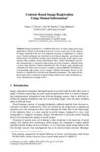
Comparison of SA techniques: We applied a known B-spline based deformation, using 5 × 5 equally spaced knots to the T2 image. Estimates of the B-Spline warp that maps the undeformed T1 image onto the deformed T2 image, were obtained using (a) Step-SA with a0 = 1500, Ai = 15 ∀i, sample-size = 5% of the total number of pixels and (b) Hybrid-SA using Samp-SA with (K0 = 2%) and step-size = 75 for the first 159 (of 2000) iterations. Step-SA was used for the later iterations with the sample size set to the average sample size of the first 159 iterations. To change the step-size smoothly, we used a0 = 75 × mini Qi159 and Ai = 1 ∀i. The two SA methods were tested using both a uniform sampling distribution and importance sampling (IS), using the sampling distribution designed in eq. (4). Thirty realisations of each of the SA methods with and without IS were obtained. Fig. 1 shows the mean performance of these SA techniques. In this and subsequent figs. error bars have been omitted to improve clarity. All +/- one standard deviation error bars were within 0.25 pixels of the mean behavior plots. Hybrid-SA with IS reduces RMS error faster than other SA configurations.
Comparison of the different SA techniques with and without IS
R.M.S. Error (pixels)
2.5
2
Hybrid−SA with IS
Hybrid−SA with a Uniform sampling distribution
Step−SA with a Uniform sampling distribution
1.5
Step−SA with IS
1
0
0.5
1
CPU Time (secs)
1.5
2 x 10
4
3. RESULTS Registration experiments used 2D 256 × 256 T1 and T2 MRI brain images obtained from the International Consortium of Brain Mapping , with pixel sizes ≈ 1mm×1mm. This pair of images was initially registered. Known deformations (ground truth) resulting in pixel coordinates given by ν(�xj ), j = 1 . . . N , were applied to the T2 image. This image was treated as the reference image, the undeformed T1 image was the homologous image. Two types of known deformation models were used: (i) a B-spline based deformation, representing zero model mismatch and (ii) a deformation generated by randomly placed gaussian blobs, not based on B-splines. The RMS error between the estimated warp given by {Tθˆ(�xj )}N j=1 and the ground truth was given by: � � N �1 � 2 RMS error = �ν(�xj ) − Tθˆ(�xj )� N j=1
448
Fig. 1. Improvement of SA techniques due to Importance Sampling Improvement due to Importance Sampling: To compare the benefits in speed afforded by IS with Hybrid-SA over commonly used deterministic gradient descent methods, we applied a known deformation made up of randomly placed gaussian blobs to the T2 image, as mentioned in (ii) above. This deformation has an inherent mismatch associated with the B-spline deformation model used to register the two images. For simplicity, registration was performed at a single resolution, using 64 intensity levels to evaluate the pdfs. The Hybrid-SA method tested both with and without IS, used Samp-SA with K0 = .5% for the first 159 of 2000 iterations. The remaining iterations used Step-SA with a0 = 20 × mini Qi159 and Ai = 1 ∀i. Deterministic gradient descent was found to perform best by using an adaptive stepsize sequence, like that of Step-SA described earlier, with
a0 = 1500 and Ai = 15 ∀i. Thirty realisations were obtained for each of the three optimization methods, with each realisation of the deterministic method intialized at a random seed point or warp guess. Fig.2 shows how the mean behaviors of the different methods compare. The Hybrid-SA method with IS shows a sharp improvement in the convergence rate.
methods, with the deterministic optimization re-initialized by a random seed point for each realisation. Hybrid-SA with IS performed well in the pyramid optimization scheme giving a large speed up in the rate of convergence.
Comparision of Hybrid−SA with deterministic gradient descent using a pyramid optimization strategy
2.6 3
2.4
Comparison of Hybrid−SA with IS and deterministic gradient descent
R.M.S. Error (pixels)
2.2
R.M.S. Error (pixels)
2.5
Hybrid−SA with a Uniform sampling distribution
Hybrid −SA with a Uniform sampling distribution Hybrid−SA with IS
1.8
2
1.6
Deterministric gradient descent with an adaptive step−size sequence
1.5
2
Deterministic gradient descent with an adaptive step−size sequence
1.4
Hybrid−SA with IS
1.2 1
1
0
500
1000
1500
2000
2500
3000
CPU time (secs) 0.5
0
500
1000
1500
2000
2500
Fig. 3. Faster convergence of a pyramid optimization scheme, using
CPU time (secs)
Hybrid-SA with IS
Fig. 2. Improvement in the speed of convergence using HybridSA with IS over deterministic gradient descent, with B-splines. The true (applied) deformation was based on randomly placed gaussian blobs.
We also incorporated the above procedures in the commonly used pyramid based B-spline registration scheme [1]. An 11 × 11 knot B-spline warp was applied to the T2 image, the T1 image was left undistorted. Our SA experiment used a 3 level pyramid: the first level used 5 × 5 knots to model the deformation, 32 intensity levels at which to approximate the pdfs and both images were downsampled by a factor of 4. Level 2 had 7 × 7 knots, 58 intensity levels and a downsampling factor of 2. The last level used 9 × 9 knots, 64 intensity levels and no downsampling. Levels 1 and 2 operated at 144 and 128 iterations of Samp-SA each. The initial sample size K0 was 1% of the total number of pixels at both levels and the step-sizes were fixed at 1 and 5 respectively. The last level used 256 iterations of Step-SA with a0 = 150, A = 1 and sample size = 5% of the total number of pixels at this level. The final warp estimate at a lower level was upsampled and used to initialise the next level. As the highest level uses only 9 × 9 knots to estimate the B-spline warp and the true (applied) warp is generated using 11 × 11 B-spline knots, there is an inherent mismatch in the registration process. The SA methods were implemented both with and without IS. The same Pyramid structure and number of iterations were used for deterministic gradient descent, which gave the best results by using an adaptive gain sequence with a0 = 10 at level 1 and a0 = 100 at levels 2 and 3. A was 1 at all levels of the pyramid. Thirty realisations were obtained for all three
449
4. CONCLUSION In these initial comparisons, the speed of convergence of SA techniques for image registration was increased by the use of importance sampling. A further improvement in the convergence rate was obtained by implementing Hybrid-SA, which is a combination of Step-SA and Samp-SA. In both the single resolution and the pyramid optimization schemes, we consistently found that Hybrid-SA with IS, accelerates convergence significantly for non-rigid image registration. The next step will be to extend this evaluation of the performance of Hybrid-SA with IS, using 3D multi-modal data sets. 5. REFERENCES [1] P. Thevenaz and M. Unser, “Optimization of mutual information for multiresolution image registration,” IEEE Trans. Image Processing, vol. 9, no. 12, pp. 2083–2099, Dec. 2000. [2] S.Klein, M.Staring, and J. Pluim, “Comparison of gradient approximation techniques for optimisation of mutual information in nonrigid registration,” Proceedings of SPIE, vol. 5747, pp. 192–203, Apr. 2005. [3] H. Robbins and S. Monro, “A stochastic approximation method,” The Annals of Mathematical Statistics, vol. 22, no. 3, pp. 41–59, Sept. 1951. [4] P. Dupis and R. Simha, “On sampling controlled stochastic approximation,” IEEE Trans. Automat. Contr., vol. 36, no. 8, pp. 915–924, Aug. 1991. [5] H. Kesten, “Accelerated stochastic approximation,” The Annals of Mathematical Statistics, vol. 29, no. 1, pp. 41–59, Mar. 1958.