Sep 20, 2007 - based value mapping (GBVM) is a technique for colorizing pixels based on value (e.g., ... dients in the image while maintaining ordinal relationships of values. GBVM is especially ..... mgg/topo/globe.html. 8. E. B. Ledford, Jr.
Journal of Electronic Imaging 16(3), 033004 (Jul–Sep 2007)
Gradient-based value mapping for pseudocolor images Arvind Visvanathan Stephen E. Reichenbach University of Nebraska–Lincoln Computer Science and Engineering Department Lincoln, Nebraska 68588-0115 Qingping Tao GC Image LLC Lincoln, Nebraska 68505-7403
Abstract. We develop a method for automatic colorization of images (or two-dimensional fields) in order to visualize pixel values and their local differences. In many applications, local differences in pixel values are as important as their values. For example, in topography, both elevation and slope often must be considered. Gradientbased value mapping (GBVM) is a technique for colorizing pixels based on value (e.g., intensity or elevation) and gradient (e.g., local differences or slope). The method maps pixel values to a color scale (either gray-scale or pseudocolor) in a manner that emphasizes gradients in the image while maintaining ordinal relationships of values. GBVM is especially useful for high-precision data, in which the number of possible values is large. Colorization with GBVM is demonstrated with data from comprehensive two-dimensional gas chromatography (GCxGC), using both gray-scale and pseudocolor to visualize both small and large peaks, and with data from the Global Land One-Kilometer Base Elevation (GLOBE) Project, using grayscale to visualize features that are not visible in images produced with popular value-mapping algorithms. © 2007 SPIE and IS&T. 关DOI: 10.1117/1.2778426兴
1 Introduction This paper develops a method for automatic colorization of images 共or two-dimensional fields presented as images兲, in order to visualize pixel values and their local differences. In many applications, such as topography, local differences in values are as important as their values. In such applications, it may be important to visually differentiate regions on the basis of both aspects—for example, in topography, to locate steep slopes in low-lying areas. Colorization commonly is used to visualize values of two-dimensional fields, but popular value-mapping methods for colorization 共such as linear mapping, surveyed in Ref. 1兲 and histogram equalization2 do not account for local differences and therefore may not effectively visualize those differences. This paper develops gradient-based value mapping 共GBVM兲 for colorization based on both pixel values and local differences for improved visualization. Two-dimensional arrays of scalar values 共such as intensity or elevation兲 commonly are displayed as images using Paper 06193R received Nov. 7, 2006; revised manuscript received Feb. 8, 2007; accepted for publication Mar. 8, 2007; published online Sep. 20, 2007. This paper is a revision of a paper presented at the SPIE Conference on Visual Information Processing XV, May 2006, Orlando, Florida. The paper presented there appears 共unrefereed兲 in SPIE Proceedings Vol. 6246. 1017-9909/2007/16共3兲/033004/8/$25.00 © 2007 SPIE and IS&T.
Journal of Electronic Imaging
a gray-scale or pseudocolor scale. Colorization maps each value of the two-dimensional array to a color specified by red, green, and blue 共RGB兲 components or, alternatively, hue, saturation, and brightness 共HSB兲 components. Let the value of the two-dimensional array p at row m, 0 ⱕ m ⬍ M, and column n, 0 ⱕ n ⬍ N, be denoted by p关m , n兴 and let the color mapping function c for the value be defined as c共p关m,n兴兲 ⬅ 共r共p关m,n兴兲,g共p关m,n兴兲,b共p关m,n兴兲兲,
共1兲
where r, g, and b are the RGB color components, each in the range 关0 , 1兴, and M ⫻ N is the image size. For a gray-scale, the RGB color components are equal for any value l: cg共l兲 ⬅ 共g共l兲,g共l兲,g共l兲兲.
共2兲
To maintain an ordinal scale, the gray-scale color components are monotonically increasing with value: if li ⬍ l j, then g共li兲 ⬍ g共l j兲.
共3兲
A discrete gray-scale may be monotonically nondecreasing 共rather than strictly increasing兲. A gray-scale image presents the smallest values as black pixels, the largest values as white pixels, and intermediate values in shades of gray with brightness increasing with value. So-called black-andwhite photography, television, and motion pictures 共which have grays as well as black and white兲 are familiar examples of gray-scale images. A gray-scale color-bar and example gray-scale image are shown on the top half of Fig. 1. A gray-scale provides a straightforward ordering of values from small to large. Unfortunately, humans may be able to distinguish fewer than 100 distinct gradations on a grayscale, so gray-scale images cannot communicate many differences among values. Pseudocolor scales can be used to visualize many more differences among values because the human visual system can discriminate more than one million colors. A pseudocolor scale allows independent functions for the three color components and the functions for color components need not be monotonically nondecreasing with value. With pseudocolor, the ordinal scale is not as straightforward as with gray-scale, but a good pseudocolor scale can commu-
033004-1
Jul–Sep 2007/Vol. 16(3)
Visvanathan, Reichenbach, and Tao: Gradient-based value mapping for pseudocolor images
mapping function兲 can result in all values mapping to a small range of colors or even to a single color. The second consideration is the allocation of the range of the color mapping function. Without prior knowledge of the distribution of values within the domain, the color mapping design may allocate discernible gradations 共i.e., the range of the mapping function兲 uniformly across the mapping domain. For example, a linear gray-scale uniformly allocates the range across the domain:
g共l兲 =
Fig. 1 A gray-scale color-bar and gray-scale image of GCxGC data 共top兲 and a cold-to-hot pseudocolor color bar and pseudocolor image of GCxGC data 共bottom兲 共color online only兲. 共To enhance visualization, the data were preprocessed for display with the nonlinear gradient-based value mapping described in this paper.兲
nicate a clear ordering of values. For example, topographic maps commonly use pseudocolor for elevation with a scale from small to large that progresses through dark blue, light blue, green, yellow, and red, with intermediate colors. This familiar pseudocolor scale, sometimes called “cold-to-hot,” also commonly is used for displaying geographic temperatures. A cold-to-hot color bar and example pseudocolor image are shown on the bottom half of Fig. 1. Pseudocolor images can present many distinguishable colors, but there is a tradeoff between having a pseudocolor scale with an ordinal progression that is simple to understand and the number of gradations that can be discerned: an easily understood scale visually differentiates a smaller number of gradations and a scale that visually differentiates a larger number of gradations makes the value ordering more difficult to understand. The design of the color mapping functions involves both its domain and range. First, because a digital display has a finite range of colors, the color mapping function must be restricted to a finite domain of values, lmin ⱕ l ⱕ lmax. Then, values outside the domain are mapped to extrema colors. For example, a gray-scale maps values less than lmin to black 共zero兲 and values greater than lmax to white 共one兲: g共l兲 =
再
0,
if l ⱕ lmin ,
1,
if l ⱖ lmax .
共4兲
If the domain of values is known in advance 共as may be the case for elevations in a particular region兲 or the values are spread across the full domain of the data type in which they are stored 共as is the case for many images stored in 8-bit unsigned integers兲, then lmin and lmax can be set to the smallest and largest expected values 共e.g., 0 and 255, respectively, for 8-bit unsigned integers兲. However, if the domain of values is not known and the domain of the data type is large 共e.g., double-precision floating point numbers兲, then an inappropriate color mapping domain 共i.e., a mismatch between the values and the domain of the color Journal of Electronic Imaging
l − lmin , lmax − lmin
if lmin ⱕ l ⱕ lmax .
共5兲
A linear mapping maintains interval scales and, if lmin = 0, also maintains ratio scales. For pseudocolor, such “uniform” allocation of gradations in a way that communicates interval and ratio relationships is less straightforward. Most familiar examples of colorized two-dimensional fields, such as elevation and temperature, are based on value only. In such images, regions of rapid local change 共e.g., a steep slope for elevation or a cold or warm front for temperature兲 should be shown with clear color transition共s兲. However, this is true only if the color mapping domain includes the data values and the color mapping range adequately distinguishes local differences in values. Ideally, a color mapping function should 共1兲 show the full domain of values and 共2兲 use its range to effectively distinguish differences between values in the domain. However, compromises are required to effectively display data with a large domain 共i.e., high-precision data兲 within the limited range of human discernment. Such compromises can be implemented in value mapping functions that are applied before colorization: c共f共p关m,n兴兲兲,
0 ⱕ f共l兲 ⬍ 1.
共6兲
Value mapping separates compromises related to the data values from the design of the color mapping function. Two approaches are popular: 共1兲 linear value mapping over a subdomain, referred to as a linear contrast stretch,1 and 共2兲 nonlinear value mapping. Histogram equalization is a wellknown nonlinear mapping that allocates the color range across the full value domain according to the probability distribution function of the values.2 Nonlinear mappings do not maintain interval and ratio scales, but can “can result in a remarkable increase in visual clarity.”3 Value mapping for colorization should take into account aspects of the data that are important for visualization; accounting only for the distribution of values may not be sufficient if local differences are also important for visualization. GBVM is motivated by the importance to many applications of visualizing local differences in images, even for high-precision data with a large domain.4 The method achieves two design goals for colorization:
033004-2
• the value mapping domain is the full domain of data values and • the value mapping function is monotonically nondecreasing 共to preserve ordinal scale兲 with the color range allocation based on local differences between Jul–Sep 2007/Vol. 16(3)
Visvanathan, Reichenbach, and Tao: Gradient-based value mapping for pseudocolor images
data values. Section 2 details computation of the GBVM function for a given image or ensemble. Section 3 demonstrates the method with data from comprehensive two-dimensional gas chromatography 共GCxGC兲. GCxGC is a powerful new technology for chemical separations that provides an order-of-magnitude increase in separation capacity over traditional gas chromatography and is capable of resolving thousands of chemical compounds.5 GCxGC data can be displayed as an image,6 as in Fig. 1, which pictures a GCxGC analysis of diesel fuel using gray-scale 共top兲 and pseudocolor 共bottom兲. 共Only a region of the data is shown.兲 Each resolved chemical substance in a GCxGC analysis produces a small blob or cluster of pixels, with values that are larger than the background values, which appear as spots. The dynamic range of GCxGC data is very large, with values of large peaks thousands of times larger than values of small peaks. Depending on the application, both small and large peaks may be important, so colorization should visualize differences 共i.e., peaks兲 across the domain of data values. Colorization can be set interactively, but the quantity and variability of GCxGC data motivate methods for automated colorization. Although GBVM was developed for visualizing GCxGC data, it also can be used for other applications, including topography, meteorology, and medical imaging. Section 3 also shows images of data from the Global Land OneKilometer Base Elevation 共GLOBE兲 Project,7 for which GBVM reveals topographic features not visible in images produced with popular value-mapping algorithms.
Fig. 2 Gradient magnitude at each pixel of the image in Fig. 1, ordered by pixel index.
ⵜ s = 冑d2x + d2y .
共9兲
For discrete data p关m , n兴, the directional derivatives are replaced by the discrete differences along columns and rows, e.g., dx ⬅ 共p关m + 1,n兴 − p关m − 1,n兴兲/2, dy ⬅ 共p关m,n + 1兴 − p关m,n − 1兴兲/2,
2
Method
This section describes how GBVM is formulated, based on pixel values and gradients. The gradient at a point in a two-dimensional field is a vector that indicates the direction of the greatest rate of change and the magnitude of the rate of change in that direction. The gradient field provides both the direction and magnitude of the steepest slope at each point. At points from which there are large local differences in data values 共i.e., steep slope兲, the gradient magnitude is large. At points from which the local differences in data values are small 共i.e., relatively flat兲, the gradient magnitude is small. In image processing, the gradient magnitude is the basis for some edge detection methods because local differences in data values indicate edges. The gradient of a continuous two-dimensional field s共x , y兲 is defined as the vector of the directional rates of change parallel to the axes: ⵜs ⬅ 关dx,dy兴,
共7兲
where dx ⬅ s / x and dy ⬅ s / y. The rate of change in any direction can be computed as the linear combination of the directional rates of change. The gradient angle ⵜ s = tan−1共dy/dx兲
共8兲
is the direction of the largest-magnitude rate of change: Journal of Electronic Imaging
共10兲
in computing the discrete gradient ⵜ. The GBVM function is computed in four steps: Step 1. The first step in computing the GBVM function is to compute the discrete gradient magnitude at each pixel of the image. Figure 2 shows the gradient magnitude at each pixel of the GCxGC image in Fig. 1, with pixels ordered sequentially by image position 共i.e., mN + n兲. For the image in Fig. 1, M = 400 and N = 3,000, for a total of 1,200,000 pixels. Step 2. The second step is to sort the pixels by their data values: 0 ⱕ orderp关m,n兴 ⬍ MN,
共11兲
such that the pixels are uniquely and correctly ordered: ∀关m,n兴 ⫽ 关m⬘,n⬘兴, ∀p关m,n兴 ⬍ p关m⬘,n⬘兴,
orderp关m,n兴 ⫽ orderp关m⬘,n⬘兴 orderp关m,n兴 ⬍ orderp关m⬘,n⬘兴,
and the data value and associated gradient of each pixel can be retrieved from the sorted array: valuep关orderp关m,n兴兴 ⬅ p关m,n兴
共12兲
gradientp关orderp关m,n兴兴 ⬅ ⵜp关m,n兴.
共13兲
This is the most computationally intensive step, but even for images as large as this example, with 1,200,000 pixels, a desktop PC 共e.g., with AMD Athlon® 64兲 can sort the
033004-3
Jul–Sep 2007/Vol. 16(3)
Visvanathan, Reichenbach, and Tao: Gradient-based value mapping for pseudocolor images
Fig. 3 Gradient magnitude at each pixel of the image in Fig. 1, ordered by pixel value.
data values in about one second. Figure 3 shows the gradient magnitude at each pixel of the GCxGC image in Fig. 1, with pixels ordered by value from smallest to largest. As would be expected for this image, pixels with larger pixel values, which form peaks, tend to have larger gradient magnitudes. Step 3. The third step is to progressively compute the cumulative gradient magnitudes 共cgm兲 for the array of pixels sorted by data value: i
cgmp关i兴 ⬅ 兺 兩gradientp关j兴兩,
0 ⱕ i ⬍ MN,
共14兲
j=0
and then scale by the reciprocal of the total gradient magnitude to compute the relative cumulative gradient magnitude 共rcgm兲: rcgmp关i兴 ⬅ cgmp关i兴/cgmp关MN − 1兴,
0 ⱕ i ⬍ MN.
共15兲
Figure 4 shows the relative cumulative gradient magnitude for sorted pixels from the image in Fig. 1. The cumulative gradient magnitude function captures how much slope is present in the data, ordered by pixel values. Indexing into the relative cumulative gradient magnitude function of the sorted array provides the fraction of the total gradient magnitude that is present at pixels having values less than or equal to the value of the indexed pixel. So, using the relative cumulative gradient magnitude function, it is possible to allocate a corresponding fraction of the color scale for all pixels with values less than or equal to the pixel indicated by the specified fraction of the total gradient magnitude. For example, in Fig. 3, the relative cumulative gradient magnitude function is 0.5 at pixel i = 1,185,573 共of 1,200,000 pixels兲 in the array of pixels sorted by value. That pixel has the value 17.10, i.e., valuep关1185573兴 = 17.10. Therefore, half of the total gradient magnitude in the image of Fig. 1 is at pixels that have a value less than or equal to 17.10. So, using half of the color scale for pixels with values less than 17.10 establishes a relationship between the cumulative gradient magnitude and the color Journal of Electronic Imaging
Fig. 4 Relative cumulative gradient magnitude at each pixel of the image in Fig. 1, ordered by pixel value.
scale while maintaining ordinal value relationships on the color scale. Step 4. The fourth and final step in computing the GBVM function is to compute the relationship between pixel value and the relative cumulative gradient magnitude. This is done by inverting the value-from-order relationship, defined in Eq. 共12兲, at control-point intervals 共to yield an order-from-value relationship兲 and then fitting the GBVM function to the relative cumulative gradient magnitude at those control points 共e.g., by linear interpolation兲. Then the input for the value mapping function is the pixel value and the output for the value mapping function is the relative cumulative gradient magnitude corresponding to that pixel value. For the example image in Fig. 1, Table 1 illustrates the relationship between the relative cumulative gradient magnitude and pixel values at intervals of one-tenth of the relative cumulative gradient magnitude and then the inverse mapping from the GBVM input 关pixel value regularized relative to the minimum and maximum data values in the image, min共p兲 and max共p兲兴: inputp共l兲 ⬅ 共l − min共p兲兲/共max共p兲 − min共p兲兲,
共16兲
to the GBVM output 共the relative cumulative gradient magnitude of the inverse of the value-from-order relationship兲: outputp共l兲 ⬅ rcgmp关value−1 p 共l兲兴.
共17兲
Figure 5 shows the GBVM function for the GCxGC image in Fig. 1 linearly interpolated between 40 control points. As seen in Fig. 1, 70% of the color scale is allocated to the smallest 5% of the pixel values because, as shown in Table 1, pixels with those values account for 70% of the total gradient magnitudes in the image. Images produced with GBVM colorization are presented in Section 3. As described here, GBVM allocates the color map at whichever values the gradient magnitudes occur and in proportion to the total gradient magnitudes at those values, so it is robust with respect to the size of the data domain and is effective for high-precision data. This is especially im-
033004-4
Jul–Sep 2007/Vol. 16(3)
Visvanathan, Reichenbach, and Tao: Gradient-based value mapping for pseudocolor images Table 1 The relationship between relative cumulative gradient magnitude and pixel value for the image in Fig. 1 is inverted at knot intervals to determine the mapping output 共relative cumulative gradient兲 as a function of the mapping input 共regularized pixel value兲. Sorted Index
Pixel Value
GBVM Input
GBVM Output
0.0
0
−0.71
0.000
0.0
0.1
999735
0.75
0.001
0.1
0.2
1115950
2.78
0.004
0.2
0.3
1156059
5.84
0.008
0.3
0.4
1174393
10.69
0.013
0.4
0.5
1185573
17.10
0.021
0.5
0.6
1193229
26.48
0.032
0.6
0.7
1197366
42.84
0.051
0.7
0.8
1199227
89.93
0.107
0.8
0.9
1199751
229.98
0.272
0.9
1.0
1200000
846.33
1.000
1.0
RCGM
portant for applications in which the data domain is large and the subdomain of the data for each image may be timevarying or unknown. 3 Results GCxGC separates chemical species with two capillary columns interfaced by two-stage thermal desorption.8 Chemicals in a sample are separated in time in each of the two columns. Then the detector 关a flame-ionization detector 共FID兲 in the example of Fig. 1兴 samples the output, producing scalar values proportional to the amounts of the constituent chemicals that are eluted at the sample time.
Fig. 5 Gradient-based value-mapping function for the GCxGC image in Fig. 1. Journal of Electronic Imaging
Fig. 6 Images with gray-scale 共left兲 and pseudocolor 共right兲 for various value-mapping functions 共color online only兲. From top to bottom: 共a兲 linear over all values; 共b兲 linear with cutoff of 0.1% tails; 共c兲 linear with cutoff of 1.0% tails; 共d兲 histogram equalization; 共e兲 gradient-based.
GCxGC data can be displayed as a digital image, with pixels arranged so that the abscissa 共x-axis, left to right兲 is the elapsed time for the first-column separation and the ordinate 共y-axis, bottom to top兲 is the elapsed time for the second-column separation. In the data of Fig. 1, each modulation for the secondcolumn separation is performed in two seconds and the data is sampled at 200 Hz for a y-axis dimension of 400 pixels. The chromatographic run time 共i.e., the time required to acquire the data with the chromatograph兲 is 100 min, with 30 modulations per minute, for an x-axis dimension of 3000 pixels, of which a little less than 30 min is shown in Fig. 1. The data values 共after baseline correction9兲 are floating-point numbers ranging from −0.71 to 846.33. Figure 1 is shown with gray-scale and “cold-to-hot” pseudocolor with the smaller values of the background colorized dark blue and the larger values of the blob peaks colorized with light blue, green, yellow, and red, indicating increasing values. As described in Section 1, a fundamental issue for colorization is the mapping domain. The domain can be defined simply by the minimum and maximum values in the data, lmin = min共p兲 and lmax = max共p兲, −0.71 and 846.33, respectively, for the example data. However, as shown in the top row of Fig. 6, simple linear value mapping over this domain shows only a few of the largest peaks clearly, shows faint spots for medium-sized peaks, and does not show small peaks at all.
033004-5
Jul–Sep 2007/Vol. 16(3)
Visvanathan, Reichenbach, and Tao: Gradient-based value mapping for pseudocolor images
Fig. 7 The histogram of the GCxGC image in Fig. 1 with log-scale x-axis.
This problem can be understood by examining the distribution of data values—the histogram, as it is called in digital image processing. Figure 7 shows the histogram of the GCxGC data shown in Fig. 1. The x-axis shows the regularized pixel values on a log scale. On a linear scale, the histogram would show only a large peak near 0, because almost 97% of the pixels have a value in the smallest 1% of the domain. So, using linear value mapping for colorization of this example utilizes only 1% of the color scale for 97% of the pixels. One approach for dealing with long-tailed distributions, such as in Fig. 7, is to reduce the domain. For example, cutting off 0.1% tails at each end of the value distribution reduces the domain to 关−0.11, 65.50兴, nearly 13-fold smaller; cutting off 0.5% tails reduces the domain to 关−0.08, 28.12兴, more than 30-fold smaller; and cutting off 1.0% tails reduces the domain to 关−0.07, 19.27兴, about 44fold smaller. Of course, one problem with this approach is how to select the size of the cutoff, but the method does yield better results. The second row of Fig. 6 shows results for 0.1% cutoff and the third row shows results for 1.0% cutoff. At 0.1% cutoff, some of the smaller peaks are visible, but many are not. At 1.0% cutoff, most of the smaller peaks are visible, but too many peaks are shown at the extreme color, causing the large and medium-sized peaks arrayed horizontally along the bottom of the image to blend together. The cutoffs at the high and low ends could be set independently, but setting the cutoffs is difficult to automate. Even if the color range is set to appropriately exclude the tails of the distributions, this approach does not account for local differences in value in the middle of the distribution, so local variations still may not be visible. Histogram equalization is an automated nonlinear valuemapping method designed to use the color scale uniformly with respect to the distribution of pixels values, i.e., each fraction of the color scale is used for a corresponding fraction of the pixels. The value mapping function is the cumulative distribution function, e.g., as shown in Fig. 7. The fourth row of Fig. 6 共the next to the last row兲 shows the images with histogram equalization. The smallest peaks at Journal of Electronic Imaging
Fig. 8 Images of elevation data from Australia for various valuemapping functions. The box in 共a兲 outlines the region displayed in 共b兲–共f兲.
the top of the image are shown clearly, much more clearly even than for linear mapping with 1.0% cutoff of the tails, and these images make visible some structure in the background 共regions without peaks兲. However, larger and medium-sized peaks along the bottom and even in the middle of the image run together and cannot be distinguished. This is because much of the color scale is used for the many pixels in the background 共even though there are insignificant differences among these pixels兲, leaving less of the color scale for pixels in peaks. Histogram equalization does not account for local differences in value and so wastes color resolution in the background where little color resolution is warranted. Colorization methods based strictly on the value distribution do not account for local differences when allocating the color range and so such differences may not be visible. Colorization with GBVM is demonstrated in the bottom row of Fig. 6. The smallest peaks near the upper right corner are more visible than in the images for linear mapping and nearly as visible as in the images for histogram equalization. The largest peaks, along the bottom of the image, are differentiated better than for linear mapping and histogram equalization. In particular, the prominent peaks for the five normal alkanes, C12 to C16, can be identified more easily. GBVM is able to show both small peaks and large peaks across the large, dynamic domain of the data because
033004-6
Jul–Sep 2007/Vol. 16(3)
Visvanathan, Reichenbach, and Tao: Gradient-based value mapping for pseudocolor images
Fig. 9 Three-dimensional perspective view of a GCxGC image colorized by gradient-based value mapping 共color online only兲.
the color range is allocated according to the cumulative gradient magnitude. So, the color mapping shows both the few large peaks with large gradients and the many small peaks with smaller gradients. GBVM was developed for GCxGC data, but can be used for other data and is especially useful for high-precision data. Figure 8 shows images with data from the GLOBE Project for Australia.7 The image is 4033⫻ 4888, two-byte signed integers, ranging from −500 共outside the mask兲 to 2431. Figure 8共a兲 shows an image with a linear gray-scale color map over the full domain of the data. A box in Fig. 8共a兲 highlights a region in South Australia north of the Spencer Gulf, which is shown in more detail in the other images. Figure 8共b兲 shows the region with full-domain linear gray-scale mapping. Figures 8共c兲–8共f兲 show, respectively, images with linear value mapping with tail cutoffs at 0.1%, linear value mapping with tail cutoffs at 1.0%, histogram equalization, and GBVM. The image produced with GBVM shows several features not visible in the images produced by the other methods, including Lake Frome in the upper right of the image and coastal flats along Spencer Gulf in the lower left of the image. 4 Conclusion Gradient-based value mapping 共GBVM兲 for colorization accounts for local value differences in allocating the color scale. The results presented here show images of diesel fuel analyzed by GCxGC-FID and elevation data for Australia. For both types of data, GBVM reveals features that are not visible in images produced by popular value-mapping algorithms. GBVM also works well for other types of data in which local differences across the range of values should be visualized and is especially useful for high-precision data. For some applications, it is important to note that any nonlinear value-mapping algorithm, such as GBVM, may not preserve interval and ratio relationships in the color scale. GBVM does maintain ordinal relationships, but intervals and ratios in the colorized images are determined by the gradient magnitudes. Nonlinear mapping functions can be combined. For example, if more emphasis of smaller peaks is desired, the data can be preprocessed with a nonlinear logarithmic value mapping prior to GBVM. Preprocessing with logarithmic mapping would reduce the relative scale of large peaks to small peaks. For applications that require comparisons between images, it is important to note that GBVM is an adaptive method that is based on an analysis of the data. If colorization should be standardized across a set of images, then Journal of Electronic Imaging
GBVM should be based on a relative cumulative gradient magnitude function computed from a representative set of images from the ensemble. Then, the same value-mapping function should be used for all images compared. GBVM also can be used to colorize three-dimensional perspective views of two-dimensional fields. Figure 9 presents a perspective view of the example GCxGC between C13 and C16. The elevation of the surface, relative to the base plane, is determined by the data value. This view clearly illustrates the large scale of GCxGC data and the effectiveness of gradient-based value mapping for visualizing large, medium-sized, and small peaks.
Acknowledgments This research was supported by the NIH National Center for Research Resources 共RR020256-01兲 and the NSF Science and Engineering Information Integration and Informatics Program 共IIS-0431119兲.
References 1. A. C. Bovik, “Basic gray-level image processing,” in Handbook of Image and Video Process, edited by A. Bovik, Academic Press, San Diego, CA, pp. 21–38 共2005兲. 2. R. A. Hummel, “Histogram modification techniques,” Comput. Graph. Image Process. 4, 209–224 共1975兲. 3. R. Hummel, “Image enhancement by histogram modification,” Comput. Graph. Image Process. 6, 184–195 共1977兲. 4. A. Visvanathan, S. E. Reichenbach, and Q. Tao, “Gradient-based value mapping for colorization of two-dimensional fields,” in Visual Information Processing, Proc. SPIE 6246, 62460I 共2006兲. 5. W. Bertsch, “Two-dimensional gas chromatography. Concepts, instrumentation, and applications—Part 2: Comprehensive twodimensional gas chromatography,” J. High Resolut. Chromatogr. 23共3兲, 167–181 共2000兲. 6. S. E. Reichenbach, M. Ni, V. Kottapalli, and A. Visvanathan, “Information technologies for comprehensive two-dimensional gas chromatography,” Chemom. Intell. Lab. Syst. 71共2兲, 107–120 共2004兲. 7. Australian Surveying and Land Information Group 共AISLIG兲 and the U. S. National Geophysical Data Center 共NGDC兲, “30 arc-second digital elevation model for Australia,” in The Global Land OneKilometer Base Elevation (GLOBE) Digital Elevation Model, edited by D. A. Hastings et al., NGDC 共1999兲. http://www.ngdc.noaa.gov/ mgg/topo/globe.html. 8. E. B. Ledford, Jr. and C. A. Billesbach, “Jet-cooled thermal modulator for comprehensive multidimensional gas chromatography,” J. High Resolut. Chromatogr. 23共3兲, 202–204 共2000兲. 9. S. E. Reichenbach, M. Ni, D. Zhang, and E. B. Ledford, Jr., “Image background removal in comprehensive two-dimensional gas chromatography,” J. Chromatogr. A 985共1兲, 47–56 共2003兲. Arvind Visvanathan is a PhD candidate in computer science at the University of Nebraska–Lincoln. He earned his BS degree in computer engineering from the University of Poona, India, in 2001, and his MS degree in computer science at the University of Nebraska–Lincoln in 2003. The topic of his master’s thesis was archiving and reporting formats for comprehensive two-dimensional gas chromatography. His current area of research is an informational theoretical approach for compound identification in comprehensive two-dimensional gas chromatography and mass spectrometry.
033004-7
Jul–Sep 2007/Vol. 16(3)
Visvanathan, Reichenbach, and Tao: Gradient-based value mapping for pseudocolor images Stephen E. Reichenbach is a professor at the Computer Science and Engineering 共CSE兲 Department of the University of Nebraska–Lincoln 共UNL兲. He earned his PhD degree in computer science from the College of William and Mary, his MS degree in computer science from Washington University in St. Louis, and his BA degree in English from the University of Nebraska. His postdoctoral positions include a National Research Council research associateship at the Visual Information Processing Laboratory, NASA Langley Research Center, and an ASEE research fellowship at the Landsat 7 Project Science Office, NASA Goddard Space Flight Center. From 1996 to 2000, he served as UNL CSE Department chair.
Journal of Electronic Imaging
He has published more than 100 journal and conference papers on digital imaging.
033004-8
Qingping Tao earned his BE degree in computer applications from Hefei University of Technology 共1997兲, his ME degree in computer software from the University of Science & Technology of China 共2000兲, and his PhD degree in computer science from the University of Nebraska–Lincoln 共2005兲. Currently, he is vice-president for research and development at GC Image, LCC.
Jul–Sep 2007/Vol. 16(3)