in a space-based application using large baffles. A small ..... with the WASSS sensor. The initial WASSS development occurred through the AF SBIR program,.
Ground testing of prototype hardware and processing algorithms for a Wide Area Space Surveillance System (WASSS) Neil Goldstein, Rainer A. Dressler, Robert Shroll, Steven C. Richtsmeier, and James McLean Spectral Sciences, Inc., Burlington, MA Phan D. Dao, Jeremy J. Murray-Krezan, and Daniel O. Fulcoly Air Force Research Laboratory, Space Vehicles Directorate, Kirtland AFB, NM ABSTRACT We report the results of observations made at Magdalena Ridge Observatory using the prototype Wide Area Space Surveillance System (WASSS) camera, which has a 4 x 60 field-of-view , < 0.05 resolution, a 2.8 cm2 aperture, and the ability to view within 4o of the sun. A single camera pointed at the GEO belt provided a continuous nightlong record of the intensity and location of more than 50 GEO objects detected within the camera’s 60 field-ofview, with a detection sensitivity similar to the camera’s shot noise limit of m v=13.7. Performance is anticipated to scale with aperture area, allowing the detection of dimmer objects with larger-aperture cameras. The sensitivity of the system depends on multi-frame averaging and a Principal Component Analysis based image processing algorithm that filters out space objects based on their different angular velocities from those of celestial objects. Results are presented for a full night of viewing on October 16, 2012. Close to 100 space objects were detected, of which ~85 were identified. 1.
INTRODUCTION
We report ground testing of a wide area camera system and automated star removal algorithms that demonstrate the potential to detect, quantify, and track deep space objects using small aperture cameras and on-board processors. The camera system, which was originally developed for a space-based Wide Area Space Surveillance System (WASSS), operates in a fixed-stare mode, continuously monitoring a wide swath of space and differentiating celestial objects from satellites based on differential motion across the field-of-view. The system would have greatest utility in a LEO orbit where it can provide automated and continuous monitoring of GEO and the GEO transfer space with high refresh rates. The ability to continuously monitor deep space enables new concepts for change detection and custody maintenance. The demonstrated detection approach is equally applicable to Earth-based sensor systems. A distributed system of such sensors, either Earth-based, or space-based, could provide automated, persistent night-time monitoring of all of deep space. The continuous monitoring provides a daily record of the light curves of all GEO objects above a certain brightness within the field-of-view. The daily updates of satellite light curves offers a means to identify specific satellites, to note changes in orientation and operational mode, and to queue other SSA assets for higher resolution queries. The data processing approach may also be applied to larger-aperture, higher resolution camera systems to extend the sensitivity toward dimmer objects. We report here the results of observations made at Magdalena Ridge Observatory (MRO) using the prototype WASSS camera, which has a 4×60 field-of-view , < 0.05 resolution, a 2.8 cm2 aperture, and the ability to view within 4o of the Sun. A single camera pointed at the GEO belt provided a continuous night-long record of the intensity and location of more than 80 GEO objects detected within the camera’s 60-degree field-of-view. The detection sensitivity of the camera was similar to the camera’s shot noise limit of mv=13.7. The performance is anticipated to scale with aperture area, allowing the detection of dimmer objects with larger-aperture cameras. The sensitivity of the system depends on multi-frame averaging and an image processing algorithm that exploits the different angular velocities of celestial objects and space objects (SO). Principal Components Analysis (PCA) is used to filter out all objects moving with the velocity of the celestial frame of reference. The resulting filtered images are projected back into an Earth-centered frame of reference, or into any other relevant frame of reference, and co-added to form a series of images of the GEO objects as a function of time. The PCA approach not only
Form Approved OMB No. 0704-0188
Report Documentation Page
Public reporting burden for the collection of information is estimated to average 1 hour per response, including the time for reviewing instructions, searching existing data sources, gathering and maintaining the data needed, and completing and reviewing the collection of information. Send comments regarding this burden estimate or any other aspect of this collection of information, including suggestions for reducing this burden, to Washington Headquarters Services, Directorate for Information Operations and Reports, 1215 Jefferson Davis Highway, Suite 1204, Arlington VA 22202-4302. Respondents should be aware that notwithstanding any other provision of law, no person shall be subject to a penalty for failing to comply with a collection of information if it does not display a currently valid OMB control number.
1. REPORT DATE
3. DATES COVERED 2. REPORT TYPE
SEP 2013
00-00-2013 to 00-00-2013
4. TITLE AND SUBTITLE
5a. CONTRACT NUMBER
Ground testing of prototype hardware and processing algorithms for a Wide Area Space Surveillance System (WASSS)
5b. GRANT NUMBER 5c. PROGRAM ELEMENT NUMBER
6. AUTHOR(S)
5d. PROJECT NUMBER 5e. TASK NUMBER 5f. WORK UNIT NUMBER
7. PERFORMING ORGANIZATION NAME(S) AND ADDRESS(ES)
8. PERFORMING ORGANIZATION REPORT NUMBER
Air Force Research Laboratory (AFRL),Space Vehicles Directorate,Kirtland AFB,NM,87117 9. SPONSORING/MONITORING AGENCY NAME(S) AND ADDRESS(ES)
10. SPONSOR/MONITOR’S ACRONYM(S) 11. SPONSOR/MONITOR’S REPORT NUMBER(S)
12. DISTRIBUTION/AVAILABILITY STATEMENT
Approved for public release; distribution unlimited 13. SUPPLEMENTARY NOTES
2013 AMOS (Advanced Maui Optical and Space Surveillance) Technical Conference, 10-13 Sep, Maui, HI. 14. ABSTRACT
We report the results of observations made at Magdalena Ridge Observatory using the prototype Wide Area Space Surveillance System (WASSS) camera, which has a 4 x 60 field-of-view , < 0.05 resolution, a 2.8 cm2 aperture, and the ability to view within 4o of the sun. A single camera pointed at the GEO belt provided a continuous night-long record of the intensity and location of more than 50 GEO objects detected within the camera?s 60 field-of-view, with a detection sensitivity similar to the camera?s shot noise limit of mv=13.7. Performance is anticipated to scale with aperture area, allowing the detection of dimmer objects with larger-aperture cameras. The sensitivity of the system depends on multi-frame averaging and a Principal Component Analysis based image processing algorithm that filters out space objects based on their different angular velocities from those of celestial objects. Results are presented for a full night of viewing on October 16, 2012. Close to 100 space objects were detected, of which ~85 were identified. 15. SUBJECT TERMS 16. SECURITY CLASSIFICATION OF: a. REPORT
b. ABSTRACT
c. THIS PAGE
unclassified
unclassified
unclassified
17. LIMITATION OF ABSTRACT
18. NUMBER OF PAGES
Same as Report (SAR)
10
19a. NAME OF RESPONSIBLE PERSON
Standard Form 298 (Rev. 8-98) Prescribed by ANSI Std Z39-18
removes the celestial background, but it also removes systematic variations in system calibration, sensor pointing, and atmospheric conditions. The resulting images are shot-noise limited, and can be exploited to automatically identify deep space objects, produce approximate state vectors, and track their locations and intensities as a function of time. The Wide Area Space Surveillance System (WASSS) was designed to meet the challenge of continuous monitoring of deep space, concentrating on rare event detection, such as GEO-insertion events, and gaining custody of objects in GEO-transfer orbits. It would also provide routine monitoring of SO, which can be used for anomaly detection and to characterize SO light curves. We have previously proposed1 a system of Low-Earth Orbit (LEO) satellites, each equipped with a number of wide area cameras that sweep out the GEO belt, providing views of deep space with refresh rates of the order of 12-24 minutes. Figure 1 shows an outline of the concept. The left side shows a system of two satellites, each with four cameras in a vertical orientation. The cameras have a 4x60 degree field-of-view, and are designed to view close enough to the sun, so that an object in GEO is always visible from one side of the earth. The right hand side shows a proposed demonstration satellite configuration with two vertical cameras and one horizontal camera. The horizontal camera would provide long term views of SO for characterization of their light curves.
Sensor FOV
Fig. 1. WASSS concept for continuous monitoring of deep space. At left, a multi-satellite system for continuous coverage using the vertical orientation. At right, a demonstration satellite with both horizontal and vertical wide area coverage. 2.
PROTOTYPE CAMERA
The WASSS prototype camera, shown in Figure 2 was designed specifically to allow viewing within 4 of the Sun in a space-based application using large baffles. A small, near-rectangular aperture of 12 x 24 mm is required to keep the baffles short to an overall length of 700 mm. The powered optics and focal plane array are enclosed in two separate chambers to further reduce scattering on the image plane. The optical design is a refinement of that used in the Solar Mass Ejection Imager (SMEI) on the Coriolis satellite2. Both systems are based on an uncorrected Schmidt camera, using a large primary mirror, M1, to project an image of a wide FOV onto a spherical field, and a secondary conical mirror, M2, to project a strip of the image into a flat image plane below M2.
Fig. 2. WASSS prototype camera system. At left, a cutaway view of solid model. At right, ray trace.
WASSS uses a second set of curved mirrors, M3 and M4, to correct image aberrations, producing a critically sampled image on the focal plane. The system is radially symmetric about the input aperture, and produces an annular image on the focal plane, as shown in Figure 3. The annular image is mapped into object field angular coordinates. The resolution is 0.028o/pixel.in the narrow field-of-view dimension (radial image field) and 0.044o in the wide field-of-view dimension (tangential image field). When properly, focused, a point source is imaged with a FWHM=1 pixel. Unfortunately, the system was not focused during the field tests, resulting in a blurred image with a range of FWHM of 2-5 pixels, depending on the location within the field-of-view. Figure 4 compares the resolution during a night sky measurement at MRO with one conducted earlier in the year at Spectral Sciences. a) Images of Point Sources
b) Transformation from Image field to Object Field
Fig. 3. Image field on DMD. a) Image of an array of point objects. b) Transformation from image to object field angular coordinates.
Fig. 4. Degradation of resolution of star imagery for the MRO field test (right) compared to imagery from October 2012 (left). 3.
MRO FIELD TEST
A series of measurements were conducted by SSI and AFRL staff at the Magdalena Ridge Observatory, MRO, during October of 2012. As shown in Figure 5, the WASSS prototype camera and electronics were placed in an aluminum box and connected to the internet for remote operation. Data were taken in two orientations, the vertical orientation with the wide field-of-view aligned along a North/South axis, and a horizontal orientation, with the wide field-of-view aligned along the GEO belt. In both orientations, the sensor was pointed at an azimuth of ~180 and a declination of ~-5.9 in order to center the field-of-view on the GEO belt.
Figure 6 shows typical image data obtained in the horizontal orientation on the night of October 14. Data were taken at a data rate of 7.5 seconds/frame, and an exposure time of four seconds. Data are reported in counts, with one count=4 photoelectrons. The raw image data is projected into the Earth centered inertial coordinate system and expressed in terms of relative RA and Dec compared to the bore sight of the sensor. The precise sensor bore sight was determined by minimizing the positional error between the known and observed locations of the stars. The residual position errors were dec=0.01o and RA=0.03o.
Fig. 5. Pictures from. the MRO Field test. Top, sensor system in the field. Middle, close-up views of the equipment box. Bottom, views of the sensor in the horizontal orientation (left) and vertical orientation (right).
Fig. 6. Raw mage data form 10:31:21 PM, October 14.
The star catalog was also used for an approximate photometric calibration, which was compared to the known camera sensitivity and optical throughput of the instrument. The integrated signal observed for the stars varied over the course of the night due to variations in cloud cover and atmospheric path. The collected photoelectron flux at the detector ranged from 25- 40% of the photon flux at the top of the atmosphere. The latter number is consistent with the estimated detector quantum efficiency, camera transmission, and atmospheric transmission. Figure 7 shows a raw data image projected into the celestial RA and Dec frame of reference.
Fig. 7. Single image from 10:31:21 registered onto a relative RA/Dec grid (intensity 1/60th of full scale)
4.
IMAGE PROCESSING
The WASSS system includes an automated data processing system that produces filtered images of deep space objects in real time. The system has the following steps: 1) 2) 3) 4) 5) 6) 7) 8) 9)
FPA image retrieval Dark background correction Projection to the RA/Dec grid Spatial smoothing Create a time series in the star frame of reference Principal component filtering to remove star background Projection to the SO frame of reference Frame averaging Generation of light curves
The basic idea, shown in Figure 8, is to create a stack of images register the images into the star field frame of reference, filter out the star background, and then re-register the images in the frame of reference of the space objects. The individual image frames (Figure 6) are first morphed into a local grid of relative RA and Dec with respect to the bore sight of the camera. The frames are stacked along the time axis to form a hypercube and then rotated about the relative declination axis to make image slices of constant RA, as shown in Figure 8. The resulting image slice depicts the transit of a star across the camera field-of-view as a function of time. Stars, which have constant RA, appear as streaks and non-celestial objects, such as SOs, appear as isolated objects. The star frame objects can be automatically subtracted using principal component analysis (PCA) filtering.
Fig. 8. Rotation of hypercube to create constant RA Frames. Image slices with constant RA are treated like vectors with multiple time components. Vectors are highly correlated between values of RA (i.e., two streaks across the image visually look similar). PCA removes these correlations and generates a set of orthogonal image projections by diagonalizing the covariance matrix generated for all of the vectors. Celestial objects are present over many vector components (long streak) and are represented by projections with high RA-variance. They are a dominant feature of the scene. Non-celestial objects do not contribute to high covariance between vectors (spot or short streak) and will be represented by projections with low RA-variance. PCA subspace projection methods were employed to isolate scene features. Subspace projections may be made based on variance discrimination (i.e. low or high RA-variance). Higher order statistics (higher moments) may also be employed to refine the separation. Here we introduce the L Factor, which is based on the fourth moment and describes the shape of the projection distributions, to further discriminate between celestial and non-celestial objects. PCA subspace projections are used to filter out regions of unwanted RA-variance. Each constant RA image slice is subject to PCA filtering to remove the correlated celestial objects, from the isolated non-celestial objects. The residual is then transformed back to the GEO frame of reference, or any other frame of reference containing a space object, as shown in Figure 9.
Fig. 9. Processing of the constant RA image slices. Clockwise from top left, constant RA image slice, principal component eigenvalues, principal component L factor, and residual image slice. The principal component number shows the maximum scene rank (124), which is the number of time elements minus one (vectors were mean subtracted).
This process is illustrated in Figures 7- 11 using the data from Figure 6. Figure 7 shows the result of the first four image processing steps. The data is background subtracted, projected onto a grid of constant RA and Dec, and spatially smoothed. The RA/Dec grid is set up so that celestial objects travel exactly one grid point between frames. The images are rotated as shown in Figure 8 and are stored in a circular buffer, on a first in first out basis. In order to minimize data latency, the image is analyzed as a set of eight, 4 x 4o sub-images, with the stars crossing each sub image from left to right in 16 minutes. The constant RA image slice shown in Figure 9 is a stack of 8 vectors, each corresponding to the RA at the right hand edge of the most recent subimage. As each image slice is completed, it is subject to principal component filtering as shown in Figure 9 and described below.
Each vector is an image slice composed of a time series of intensity values for constant RA. Data are arranged into a matrix X, which is an N pixel × M time representation. Xij is a single value for time i and pixel j. The mean for each image j is thus,
the mean subtracted data set is given by,
and the covariance matrix is defined by,
The eigenvectors of the covariance matrix, A, diagonalize the matrix and provide a set of orthogonal image slices (linear combinations of the original image slices),
with a diagonal covariance matrix, which are the matrix eigenvalues or equivalently variances over the orthogonal vectors,
Two metrics are used to assign the principal components to either star components or to residual components. The first is the variance (eigenvalue). As mentioned previously, celestial objects have higher variance than non-celestial object, sensor pattern noise, and white noise. A second, optional metric is a temporal localization factor, Lj, computed from the sum of the fourth power of the eigenvectors,
where a is a column of A. The eigenvectors a have zero mean and unit variance. They follow the temporal character of image elements (objects, sensor noise, etc.). For non-celestial objects, a few temporally isolated values cause a similar response in the eigenvector, which will preferentially weight the image slices representing the object. The sum of eigenvector elements taken to the fourth power will be significantly increased compared to a Gaussian distribution. For celestial objects, the distribution of values is more closely Gaussian. Thus, Lj is highest for objects that are highly temporally localized. The additional metric may be used to discriminate between celestial and noncelestial object with similar RA-variance. The algorithm is applied as a clutter rejection filter. For instance, the Yj highest value variance may be used to project out a new image representing the celestial objects.
In general, a may have any subset of the columns of A (e.g. all columns associated with a variance cutoff). If all columns are included then AAT = 1, and the projection leaves the image unchanged. This is a specific example of a simple and robust re-ordering algorithm and it is a straight forward process to introduce others. A threshold may be set for the variance values and/or Lj values to determine the subset of Yj images that should be used for detection providing an ordered list of Yj images with Lj values and/or variance above those representing white noise. This factor Li, which is also plotted in Figure 9, has a value of 1 for a temporally isolated event. For a random temporal distribution, it reaches a limit of sqrt(2/N), where N is the number of principal components. This function behaves in a similar way to the negentropy function for the power projected image3, but requires much less computation, and thus is more suitable for the real-time filtering system. Figures 9- 11 show typical results using just a variance filter set with a threshold of 20 times the median variance ro filter out celestial objects. The median variance is typically equal to or slightly larger than the random noise in the input data; in this case the random noise is given by the shot noise on the sky background. The components associated with the star streaks typically have much higher variance due to the larger intensity of the stars. There are typically 10 or so principal components with variance above the threshold, and these contain most of the intensity of the stars, and little of no intensity from weak SOs. The filtered residual, shown in Figure 9 contains most of the SOs which appear as short streaks, along with some time varying signal from the bright stars that alternates in sign. When transformed back into the SO frame of reference, we see a small residual in the individual frame image shown in Figure 10. When averaged together over a three minute interval (24 frames), as shown in Figure 11, the time varying signal averages out, leaving an image that is very near to the shot noise limit.
Fig. 10. Residual image from 10:31:21 (intensity 1/6000th of full scale).
Fig. 11. Three-minute average of residual image 10:28:21- 10:31:21 (intensity 1/12000th of full scale). The variance filter alone is sufficient for separating weak SOs from the star background. However, if we want to measure the intensity of moderate to strong SOs, it helps to include the second factor, Li, to avoid assigning the signal from bright SOs to the star field. In cases where the glint from the SO approaches the intensity of the stars, the first few principal components often contain most, if not all of the SO intensity. In that case, we used the Li factor to identify the temporally isolated SOs. Typically, we set a threshold of Li < 0.175, to distinguish the SOs. All vectors with an Li value higher than the threshold are assigned to the residual. This results in a somewhat higher star background, but allows us to capture the light curves of SO objects even when they are the brightest object in the scene. 5.
LIGHT CURVES OF GEO OBJECTS
Some 100 objects are readily observable in the residual images. To date we have identified about 85 objects based on their published element sets. The objects can be classified into four categories: 1) geostationary satellites, 2) higher inclination GEO active and inactive satellites, 3) objects with high longitudinal drift rates, mostly rocket bodies, and 4) terminator pass LEO objects. Figure 12 is an 8-hour average image where the brightest objects are actively controlled GEO-stationary objects along the GEO belt (category 1). In addition we see a significant number of higher-inclination GEO objects that pass through the field-of-view over a period of hours. The significant number of inactive satellites can be attributed to the 105 W geopotential well near the center of the field-of-view. Figure 13 shows a set of images, each collected with 3 minute averages, showing a number of moving objects that pass through the field-of-view. Of the four highlighted moving objects, two have not been identified and are possibly objects for which element sets are not available in the public NORAD catalog. . (from left to right) XM-3 AMC-16 XM-5 NIMIQ 4 BRASILSAT B4
AMC-9
SES-2
SPACEWAY 3 G-3C
G-17 NIMIQ 2 NIMIQ 6
G-28
G-16 DIRECTV 11 SPACEWAY 2
DIRECTV 8 SES-1 DIRECTV 9S DIRECTV 4S
ECHOSTAR 17 ANIK F1R ANIK F1
G-23 ECHOSTAR 9
VIASAT-1 BLUES XM-1
SATMEX-6 SIRIUS FM-5
ECHOSTAR 7 ECHOSTAR 14 DIRECTV 7S
WILDBLUE-1 ANIK F2
AMC-18 AMC-15
G-19
G-25
ECHOSTAR 11 DIRECTV 5 ECHOSTAR 10
G-18
G-13
G-14 AMC-21
AMC-11
CIEL-2 G-12
SATMEX-5
DIRECTV 12 DIRECTV 10 SPACEWAY 1 AMC-1 SES-3
Fig. 12. 8-hour average of residual showing the location of GEO objects
Fig. 13. 3-minute average images showing the motion of three SOs through the field-of-view. SOs are marked with a yellow circle and, the first two from left to right, have been identified as Thuraya 1 (inactive) and Inmarsat 4F3 (active). The other two have not been identified with objects listed in the public catalog. We have made preliminary measurements of the intensity evolution of the identified objects, using the published ephemeris data to track the objects through the field-of-view. Figures 14 and 15 show typical results for a bright controlled object at low inclination, AMC 9, and for an uncontrolled, inactive object, Solidaridad 2, drifting through the field-of-view. The algorithm tracks the integrated intensity in the area around the predicted trajectory of the object and averages the data over 1 minute with a sliding smooth. Figure 14 shows the data in integrated counts as a function of time of day. Figure 15 presents the same data as light curves on a visual magnitude versus solar phase angle scale. The active AMC-9 satellite clearly exhibits a strong glint at a phase angle of 6. The inactive satellite enters the field-of-view at a phase angle of ~12, and has highly variable intensity that diminishes with increasing phase angle.
Fig. 14. Time histories for AMC 9 (active GEO) and Solidaridad 2 (inactive, high inclination GEO).
Fig. 15. Light curves extracted for AMC 9 (active GEO) and Solidaridad 2 (inactive, high inclination GEO).
6.
SIGNAL TO NOISE CONSIDERATIONS
The residual imagery data and light curves show large areas with random noise equivalent to the shot noise of the sensor, with occasional spikes due to star residuals. The random noise is dominated by the sky background, which has a typical magnitude of 1800 e-/pixel (or 450 counts/pixel) in a raw image obtained with a 4 second exposure. After spatial smoothing and time averaging, the shot noise limit for a 3 minute average image (24 frames), such as Figures 11 and 13, is about N= 1 counts, which is equal to the observed random noise in the imagery data. Based on the star-based radiometric calibration this corresponds to a visual magnitude of mv =13.7. For the one-minute averaged light curves, which are summed over 9 grid points, the shot-noise level should be about N= 6 counts. Based on the star-based radiometric calibration this would correspond to a visual magnitude of mv =14.3. The observed standard deviation of the light curves of weak SOs ranges from =8 counts (mv=14.6) to =16 counts (mv =13.8), which suggests some residual non-random noise component introduced by the processing. The larger values typically arise from bright stars passing through the field-of-view. Star residuals are typically about 0.2% of the total star signal. Thus, stars with intensities higher than mv=7 leave a noticeable residual. Such star interference events, however, are relatively rare, and can readily be identified. 7.
CONCLUSIONS
We have demonstrated a small aperture, wide field-of-view deep space staring sensor that simultaneously observes a large number of space objects in deep space. The automated processing of imagery results in near-shot noiselimited removal of the star background. The residual noise level is equivalent to about mv=14 for averaging times of the order of 1 minute. The WASSS system sensitivity is limited by the small aperture area of A=2.5 cm2. The presented processing techniques should also be applicable to data collected with larger aperture optical systems resulting in lower limits of detection. ACKNOWLEDGMENTS The authors are grateful to Eileen Ryan, Bob Ryan, and the MRO staff for their support of the WASSS field experiments. The authors would also like to thank Andrew Buffington, and Bernard Jackson for helpful discussions associated with the WASSS sensor. The initial WASSS development occurred through the AF SBIR program, contract FA9453-10-C-0062. REFERENCES 1. N. Goldstein, R. A. Dressler, E. Perillo and R. S. Taylor, Report No. AFRL-RV-PS-TR-2012-0015, (2012). 2. C. J. Eyles, G. M. Simnett, M. P. Cooke, B. V. Jackson, A. Buffington, P. P. Hick, N. R. Waltham, J. M. King, P. A. Anderson and P. E. Holladay, "The Solar Mass Ejection Imager (SMEI)," Solar Physics 217 (2), 219-347 (2003). 3. A. Hyvarinen, "Fast and Robust Fixed-Point Algorithms for Independent Component Analysis," IEEE Trans. on Neural Networks, 10(3), (1999).