Growing multiplex networks

Growing multiplex networks V. Nicosia,1 G. Bianconi,1 V. Latora,1, 2 and M. Barthelemy3

arXiv:1302.7126v3 [physics.soc-ph] 31 Jul 2013

1

School of Mathematical Sciences, Queen Mary University of London, Mile End Road, E1 4NS, London (UK) 2 Dipartimento di Fisica e Astronomia, Universit` a di Catania and INFN, 95123 Catania, Italy 3 Institut de Physique Th´eorique, CEA, CNRS-URA 2306, F-91191, Gif-sur-Yvette, France We propose a modelling framework for growing multiplexes where a node can belong to different networks. We define new measures for multiplexes and we identify a number of relevant ingredients for modeling their evolution such as the coupling between the different layers and the distribution of node arrival times. The topology of the multiplex changes significantly in the different cases under consideration, with effects of the arrival time of nodes on the degree distribution, average shortest path length and interdependence. PACS numbers: 89.75.Fb, 89.75.Hc and 89.75,-k

Many different physical, biological and social systems are structured as networks, and their properties are now, after a decade of efforts, well understood [1–4]. However, a complex network is rarely isolated, and some of its nodes could be part of many graphs, at the same time. Examples include multimodal transportation networks [5, 6], climatic systems [7], economic markets [8], energy-supply networks [9] and the human brain [10]. In these cases, each network is part of a larger system in which a set of interdependent networks with different structure and function coexist, interact and coevolve. So far network scientists have investigated these systems by looking at one type of relationship at a time, e.g., by analyzing collaboration networks and email communications as separate graphs. However, the structural properties of each of these networks and their evolution can depend in a non-trivial way on that of other graphs to which they are interconnected. Consequently, these systems are better represented as multiplexes, i.e. graphs composed by M different layers in which the same set of N nodes can be connected to each other by means of links belonging to M different classes or types. Despite some early attempts in the field social network analysis [11], the characterization of multiplexes is still in its infancy, mainly due to the lack of multiplex data. However, some recent works have already proposed suitable extensions to multi-layer graphs of classic network metrics and models [12–14]. Preliminary results show that multiplexicity has important consequences for the dynamics of processes occurring in real systems, including routing [12, 15], diffusion [16], cooperation [17], election models [18], and epidemic spreading [19]. Nowadays, an increasing number of new data sets of multiplex systems, e.g. coming from large online social networks [20, 21], trading networks [22] and human neuroimaging techniques [23], are rapidly becoming available and demand for adequate models to understand their structure and evolution. In this Letter we propose and study a generic model of multiplex growth, inspired by classical models based on preferential attachment, in which the probability for a newly arrived node to establish connections to existing

nodes in each of the layers of a multiplex is a function of the degree of other nodes at all layers. We define two new metrics to characterize the structure of multiplexes and we study the effect of different attachment rules and the impact of delays in the arrival of nodes at different layers on the structure of the resulting network. We provide closed forms for both the degree distributions at each layer and the inter-layer degree-degree correlations, and we show how different attachment kernels can change the distributions of distances and interdependence. More precisely, a multiplex is a set of N nodes which are connected to each other by means of edges belonging to M different classes or types. We represent each class of edges as a separate layer, and we assume that a node i of the multiplex consists of M replicas, one for each layer. We denote by V [α] the set of nodes in layer α and by E [α] the set of all the edges of a given type α. An M -layer multiplex is therefore fully specified by the vector A = [A[1] , A[2] , . . . , A[M] ], whose elements are the [α] [α] adjacency matrices A[α] = {aij }, where aij = 1 if node i and node j are connected by an edge of type α, whereas P [α] [α] [α] aij = 0 otherwise. We denote by ki = j aij the degree of node i at layer α, i.e. the number of edges of type α of which i is an endpoint, and by ki the M -dimensional vector of the degrees of the replicas of i. In general, the degrees of the replicas of i are distinct, and some replicas [α] can also be isolated (i.e. ki = 0 for some value of α). In the following we consider all the edges at all layers to be undirected and unweighted. As in the case of classical ‘singlex’ graphs, we can characterize each layer α of a multiplex by studying the degree distribution P (k [α] ), [α] and the joint-degree distribution P (k [α] , k ′ ). However, we are interested here in the structural properties of the multiplex as a whole, so we propose to quantify the correlations between the degrees of replicas of the same node at two different layers α and α′ , by constructing the inter′ layer joint-degree distributions P (k [α] , k [α ] ), or the con′ ditional degree distributions P (k [α ] |k [α] ). In particular, we can look at the projection of the conditional distribu′ tion obtained by considering the average degree k¯[α ] at

2 layer α′ of nodes having degree k [α] at layer α: X ′ ′ ′ k¯[α ] (k [α] ) = k [α ] P (k [α ] |k [α] )

(1)

k[α′ ]

By plotting this quantity as a function of k [α] we can detect the presence and the sign of degree correlations between the two layers. For a multiplex with no correlations ′ ′ between layers α and α′ we expect k¯[α ] (k [α] ) = hk [α ] i ′ ′ and k¯[α] (k [α ] ) = hk [α] i. If k¯[α ] (k [α] ) increases with k [α] we say that the degrees of the two layers have positive ′ (assortative) correlations, while if k¯[α ] (k [α] ) is a decreasing function of k [α] we say that the degrees on layer α and α′ are anticorrelated (or disassortatively correlated). We notice that a similar concept of inter-network assortativity was already defined in Ref. [24] for the case of interdependent graphs, while the authors of Ref. [13] proposed to measure inter-layer assortativity by means of the Pearson’s linear correlation coefficient of degrees [25]. 300

0

10

b)

a) -3.0

~k

-2

10

k ~ m(k+2)/(m+1)

200

-4

10

100

-6

k(k)

10

0 300

P(k)100 -2

-3.0

10

200

k~k

~k

-4

10

100

-6

10

10

k 100

1000 0

100

k

200

0 300

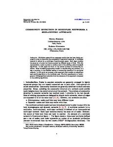
FIG. 1. (color online) Synchronous linear attachment. Panel a-b: the degree distribution P (k) (left) and the projec¯ tion k(k) of the inter-layer degree correlations (right) closely follow the theoretical curves (solid black lines) and are relatively insensitive to the coupling matrix.

In addition to the assortativity, we can also characterize the ‘multiplex reachability’ of a node i, e.g., by computing the average distance Li from i to any other node of the multiplex, and comparing this average distance with that measured on each layer separately. The presence of more than one layer in a multiplex produces an increase in the number of available paths, so that the distance between two nodes of a multiplex will be, in general, smaller than or at most equal to that measured on each layer separately. A better measure to quantify the value added by the multiplexicity to the reachability of nodes is the interdependence [12] which for a node i is defined by λi =

X ψij j∈N

j6=i

σij

(2)

where ψij is the number of shortest paths between node i and node j which use edges lying on more than one layer, while σij is the total number of shortest paths between i and j in the multiplex. The interdependence of a multiplex is computed as the average node interdependence P λ = 1/N i λi with λ ∈ [0, 1]. If λ is close to zero, then most of the shortest paths among nodes lie on just one layer, while if λ is close to 1 the majority of the shortest paths exploit more than one layer. The few models of multiplexes proposed so far are based on the juxtaposition of random graphs [13]. However, networks usually result from a growing process consisting in the addition of nodes and edges over time. For this reason, we introduce here a model of growing multiplex networks. Most of the classical growing models for single-layer networks start from an initial connected graph with m0 nodes and assume that new nodes arrive in the graph one by one, carrying m edge stubs, and connect with other existing nodes according to a prescribed attachment rule. In that case, each node i has a unique arrival time ti , but in multiplexes, instead, each layer can exhibit a different edge-formation dynamics, and in general the edges of the M replicas of a new node are not created at the same time. For instance, a face-toface interaction relationship is usually established before two individuals become friend, while two locations are usually connected by a road before a direct railway line between them is constructed. Consequently, we assume that a newly arrived node has exactly m stubs on each layer of the multiplex (in Appendix we briefly discuss the case where m is a random variable), but the replica of a node i on layer α can connect its m stubs at a different [α] time ti . We denote by ti the vector of arrival times of the replicas of node i. In order to make the model analytically tractable, we make two simplifying assumptions. The first is that there exists a layer α ¯ so that [α] [α] ¯ ¯ This is equivalent to saying that ti ≤ ti ∀i, ∀α 6= α. a newly arrived node must first create its connections on layer α ¯ before any of its replicas can create connections on any other layer α 6= α ¯ . We call α ¯ the master layer (in Appendix we briefly discuss the case in which this assumption does not hold, and each node can arrive first on any of the M layers of the multiplex). The second assumption is that nodes arrive one by one on the master layer, at equal discrete time intervals t = {1, 2, . . . , }. We label the nodes of a growing multiplex according to the ordering induced by their arrival on the master layer. Without loss of generality, in the following we assume that the the master layer is the first one, i.e. α ¯ = 1, and that the arrival times of the replicas of node i have the form [α]

ti

[1]

= T (ti , ξ [α] (τ )) [1]

(3)

where T is a certain function of ti and of the random variable ξ [α] (τ ). By appropriately choosing T and ξ [α] (τ )

3 0

10

a)

-3

c)

10

d)

0.1

0.1

P(k) -6

10 0 10

P(Li) ~k

-3

10

P(λi)

0.05

-3

0.05

-6

10

1 1000

100

k(t)

10

100

1000

2

3

Li 4

5

0.6

λ0.8 i

b) 1

1.5

e)

β=1.1 β=1.5 β=2.0 β=2.5

δ 0.55 0.5 2

1000

100

0

1.5

2

40%

45%

0

0.2

P(Hi) 0.1

δ 0.55 0.5 1

1

50%

55%

0 60%

Hi

t

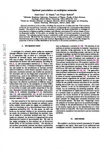
FIG. 2. (color online) Delayed linear attachment. (a) Degree distribution on the first layer. When β is close to 1, super-hubs appear. (b) The degree k(t) of the largest hub of the first layer as a function of time scales as (t/t0 )δ , where δ approaches 0.5 when β increases (insets). The value of β tunes the shape of the distribution of average shortest path lengths (c) and node interdependence (d). (e) The percentage of times Hi that the maximal-degree node in a shortest path from node i belongs to the first layer. When β is small, superhubs in the first layer are more abundant in the shortest paths.

we can model different arrival behaviors, including a) si[1] multaneous arrival (T = ti ); b) power-law delayed ar[1] rival (T = ti + ξ(τ ) and P (ξ = τ ) = (β − 1)τ −β for τ ≥ 1 and β > 1). Upon arrival, the newborn node i connects to m existing nodes in the master layer, according to a certain attachment rule. As in the preferential attachment models [27], we assume that the attachment probability depends on the degree of a node. However, in a multiplex the probability for node i to connect to [α] node j on each layer α can depend not only on kj but also on the degrees of j’s replicas on the other layers [α]

Fj (kj ) [α] Πi→j = P [α] l Fl (kl )

(4)

For the sake of clarity and without loss of generality, we focus in the following on 2-layer multiplexes with α = 1, 2. We begin with the simplest case of linear attachment which is the natural extension of the Barab´ asiAlbert model [27]. In this case, we consider that the probability for a newborn node i to connect to an existing node j on layer α is proportional to a linear combination of the degrees of j at all layers. The attachment kernels can then be expressed as  [1]     [1,1] [1,2]  F [k, q] k c c k = C = [2,1] [2,2] (5) q q F [2] [k, q] c c where we use here and in the following the notations k [1] = k and k [2] = q [28]. The coefficients c[r,s] tune the dependence of the attachment probability at layer r on the degrees of nodes at layer s. In the

case of 2-layer multiplexes we can represent the set of coefficients C = {c[r,s] } using the compact notation {c[1,1] , c[1,2] , c[2,1] , c[2,2] }. The dynamics can be easily solved in mean-field (see Appendix for details) and in some specific cases we can fully characterize the degree correlations within the two different layers by analytically solving the master-equation. If we denote by Nk,q (t) the number of nodes having, at time t, degree k on the first [α] layer and degree q on the second layer, and by Πk,q the probability that one of these Nk,q (t) nodes acquires one of the m new links on layer α at time t + 1, the master equation can be written as [29] Nk,q (t + 1) = Nk,q (t) + G − L

(6)

where h i [1] [2] G = m Πk−1,q Nk−1,q (t) + Πk,q−1 Nk,q−1 (t) + δk,m δq,m i h [1] [2] L = m Πk,q + Πk,q Nk,q (t)

represent, respectively, the expected increase (G) and the expected decrease (L) of Nk,q at time (t + 1). Assuming that Nk,q = tP (k, q) for large t, the solution of Eq. (6) is obtained by solving the corresponding recursive expression (see Appendix for details). In the following we summarize the master-equation solution in some particularly interesting cases. First of all let us consider simultaneous arrival of the nodes in the two layers. If we set C = {1, 0, 0, 1} then the attachment probability at each layer will depend only on the degree of the nodes in the same layer. In this case the degree distribution in the first layer reads [30, 31] P (k) =

2m(m + 1) , k(k + 1)(k + 2)

k>m

(7)

and the degree distribution in the second layer is identically equal. This distribution goes as P (k) ∼ k −γ with γ = 3. If we solve the master-equation for the multiplex evolution we obtain the analytical expression for the inter-layer joint degree probability P (k, q) 2Γ(2 + 2m)Γ(k)Γ(q)Γ(k + q − 2m + 1) Γ(m)Γ(m)Γ(k + q + 3)Γ(k − m + 1)Γ(q − m + 1) (8) ¯ The average degree k(q) at layer 1 of nodes having degree q at layer 2 reads:

P (k, q) =

m(q + 2) ¯ k(q) = 1+m

(9)

Notice that even if the two layers grow independently, the simultaneous arrival introduces non-trivial inter-layer degree correlations. In fact, in the mean-field approach, the degree of a node on each layer increases over time 1/2  [α] [α] (see Appendix for details), so as ki (t) = m t/ti

4 0

10

a)

-2

10

P(k) -4

10

b) k(k)

2

10

1

10

10

0.1

k

c)

100

10 0.9

100

10

P(λi) 0.1

0.05 0.7 3

4

Li

0

5000

t

10000

0 0.6

k

e)

0.2

λ(t)

P(Li)

k

d)

0.8

λi

100

{0,1,0,1} {0,1,1,0} {0,1,1,1} {1,0,0,1} {1,0,1,0} {1,0,1,1} {1,1,0,1} {1,1,1,0} {1,1,1,1}

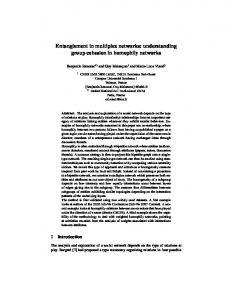
FIG. 3. (color online) Semi-linear attachment. Degree distributions (a) and inter-layer degree correlations (b) for semi-linear attachment. (c) The distribution of the average shortest path length from one node to all the other nodes heavily depends on the coupling pattern. Similarly, the interdependence of a node λ(t) is always a sublinear function of the arrival time t but its shape depends on the coupling pattern at work (d). In general, older nodes have smaller interdependence. (e) The coupling pattern also affects the distribution of node interdependence. The smallest average interdependence is observed when the two layers are independent (yellow curve).

nel which allows to grow multiplexes in which the two layers have different topological structures. The model is defined as follows  [1]    F [k, q] k = C (10) 1 F [2] [k, q] where C is still a 2 × 2 matrix of coefficients, as in the linear model. In this case, the degree of a node on any of the two layers could depend only on its degree on layer 1 and does not ever depend on its degree on layer 2. If we set C = {1, 0, 0, 1} we can analytically solve the master equation and the degree distributions of the two layers read: P [1] (k) ∼ k −3 ,

(11)

while the inter-layer joint degree distribution is equal to P (k, q) = a(k)

k−m X  n=0

where a(k) = given by

 q−m+1 2m k − m (−1)k−m+n n 2 + 2m + k − n (12)

Γ(k) Γ(m+1)Γ(k−m+1) .

¯ k(q) =m that the degrees of the two replicas of a node i depend, for large t, only on their arrival time. If both replicas have [2] [1] the same arrival time, i.e. ti = ti then the degree of the two replicas will be positively correlated. In Fig. 1 we ¯ report the degree distribution and the values of k(q) for two coupling patterns, which are in good agreement with the theoretical curves [32]. It is clear from the figure that in the synchronous arrival case the shape of the coupling matrix is actually not very relevant and that the value of the degree distribution exponent and strong assortativity are robust features of these multiplexes. If we consider a power-law delayed arrival time on the second layer, the results are significantly different. In Fig. 2 we illustrate how the exponent of the delay distribution β affects the structure of the obtained multiplex. The bulk of the degree distributions are still power laws P (k) ∼ k −γ with γ = 3, but the shape of the far tail depends now on β: for small β, a few nodes are predominant and become super-hubs (as also shown in Fig. S-1 in Appendix). The average shortest path and the interdependence are also significantly affected, as shown in Fig. 2c-d. In particular, when β is closer to one the presence of more predominant ‘old’ hubs lowers the average shortest path and the inter-layer assortativity. Moreover, broader delays cause a lower participation of hubs of the second layer in shortest paths, as shown in Fig. 2e. So far we have considered the case of two scale-free growing networks, but it would be interesting to construct multiplexes in which a scale-free network is coupled to a network with a peaked degree distribution. In this respect, we introduce a semi-linear attachment ker-

P [2] (q) ∼ e−q



2(m + 1) 1 + 2m

¯ The function k(q) is q−m+1

(13)

Similar relations can be derived for the other coupling patterns. In Panel a) and b) of Fig. 3 we report the ¯ degree distribution and the value of k(q) for three different coupling patterns, which are in good agreement with the theoretical curves. In the semi-linear model the coupling pattern has a dramatic impact on other structural properties of the multiplex such as the distribution of the average shortest path length from each node and the distribution of node interdependence. In particular, the interdependence is smaller for older nodes, and grows sublinearly with time. This implies that navigation for old nodes is easier within a single layer while younger nodes will have to resort to the different layers to reach a target. In addition, a sublinear growth implies that the system performance increases very slowly. V.N. and V.L. acknowledge support from the Project LASAGNE, Contract No.318132 (STREP), funded by the European Commission. M.B. thanks Queen Mary University of London for its warm welcome at the start of this project, and is supported by the FET-Proactive project PLEXMATH (FP7-ICT-2011-8; grant number 317614) funded by the European Commission.

[1] R. Albert and A.-L. Barabasi, Rev. Mod. Phys. 74, 47 (2002). [2] M. E. J. Newman, SIAM Review 45, 167–256 (2003). [3] S. Boccaletti, V. Latora, Y. Moreno, M. Chavez and D.U. Hwang, Phys. Rep. 424, 175–308 (2006).

5 [4] A. Barrat, M. Barthelemy and A. Vespignani, Dynamical Processes on Complex Networks (Cambridge University Press, Cambridge, England, 2008). [5] M. Kurant and P. Thiran, Phys. Rev. Lett. 96, 138701 (2006). [6] S.-R. Zou, T. Zhou, A.-F. Liu, X.-L. Xu and D.-R. He, Phys. Lett. A 374, 4406–4410 (2010). [7] J. Donges, H. Schultz, N. Marwan, Y. Zou and J. Kurths, Eur. Phys. J. B 84, 635–651 (2011). [8] J. Yang, W. Wang and G. Chen, Physica 388A, 2435– 2449 (2009). [9] S. V. Buldyrev, R. Parshani, G. Paul, H. E. Stanley and S. Havlin, Nature (London) 464, 1025–1028 (2010). [10] E. Bullmore and O. Sporns, Nat. Rev. Neurosci. 10, 186– 198 (2009). [11] S. Wasserman and K. Faust Social Network Analysis (Cambridge University Press, Cambridge, 1994) [12] R. G. Morris and M. Barthelemy, Phys. Rev. Lett. 109, 128703 (2012). [13] K.-M. Lee, J. Y. Kim, W. kuk Cho, K.-I. Goh and I.-M. Kim, New J. Phys. 14, 033027 (2012). [14] G. Bianconi, Phys. Rev. E 87, 062806 (2013). [15] Y. Zhuo, Y. Peng, C. Liu, Y. Liu and K. Long, Physica A 390, 2401–2407 (2011). [16] S. G´ omez, A. D´ıaz-Guilera, J. G´ omez-Garde˜ nes, C. J. P´erez-Vicente, Y. Moreno and A. Arenas, Phys. Rev. Lett. 110, 028701 (2013). [17] J. G´ omez-Garde˜ nes, I. Reinares, A. Arenas and L. M. Flor´ıa, Sci. Rep. 2, 620 (2012). [18] A. Halu, K. Zhao, A. Baronchelli and G. Bianconi, EPL– Europhys. Lett. 102, 16002 (2013). ´ Serrano and M. Bogu˜ [19] A. Saumell-Mendiola, M. A. n´ a, Phys. Rev. E 86, 026106 (2012). [20] M. Szell, R. Lambiotte and S. Thurner, Proc. Natl. Acad. Sci. USA 107, 13636 (2010). [21] M. Magnani, B. Micenkova and L. Rossi, preprint, arXiv:1303.4986 (2013). [22] M. Barigozzi, G. Fagiolo and D. Garlaschelli, Phys. Rev. E 81, 046104 (2010). [23] V. Nicosia, M. Valencia, M. Chavez, A. D´ıaz-Guilera, V. Latora, Phys. Rev. Lett. 110, 174102 (2013). [24] R. Parshani, C. Rozenblat, D. Ietri, C. Ducruet and S. Havlin, EPL–Europhys. Lett. 92, 68002 (2010). [25] Notice that, as shown in [26], the Pearson’s coefficient becomes infinitesimal in N when degree fluctuations are unbounded (e.g., in the case of power-law distributions P (k) ∼ k−γ with γ < 3), so that it should not be employed to accurately quantify degree correlations in a generic scale–free network. [26] N. Litvak and R. van der Hofstad, Phys. Rev. E 87, 022801 (2013). [27] R. Albert, H. Jeong and A.-L. Barabasi, Nature 401, 130–131 (1999). [28] It is easy to show that the time required to simulate the growth of a multiplex with N nodes and M layers increases as O(N 2 M ). See Appendix for additional details [α] [29] Notice that for t ≫ 1 we have Πk,q ≪ 1 ∀k, q; consequently, aymptotically in time we can neglect the probability that the same node acquires, at time t, a link in layer 1 and in layer 2. [30] S. N. Dorogovtsev, J. F. F. Mendes and A. N. Samukhin, Phys. Rev. Lett. 85, 4633 (2000). [31] P. L. Krapivsky and S. Redner, Phys. Rev. E 63, 066123

(2001). [32] All the results shown in the figures correspond to 2-layer multiplexes with N = 10000 nodes, m = 3, m0 = 3, and are averaged over 50 realizations.

6 Mean-field theory

In this section, using a mean-field approach, we discuss the time evolution of the degree of the nodes of a multiplex in the different layers and we derive long-time expressions for the degree distribution at each layer and for the interlayer degree-degree correlations. We first consider the linear attachment case (A) and then proceed to the semi-linear case (B). We also provide a concise discussion of the case in which new nodes bring a random number of new edges (C). Linear attachment kernel on both layers

According to the growth model discussed in the main text, the probability that a newly arrived node i in the multiplex creates a link to node j on layer α can be written as [α]

Fj (kj ) [α] Πi→j = P [α] l Fl (kl )

[α]

(S-1) [α]

where Fj (kj ) is a certain function of the degrees of the replicas of node j. If Fj (kj ) is a linear function of kj ∀α, and all the replicas of the new node arrive at the same time, the temporal evolution of the degree of a node on each layer is governed by the equations " [1] #     [1] dk 1 c[1,1] c[1,2] k [1] 1 k dt (S-2) = C [2] = dk[2] k 2t 2t c[2,1] c[2,2] k [2] dt with the constraints c[1,1] + c[1,2] = 1 and c[2,1] + c[2,2] = 1. Since the matrix elements are real and non-zeros, the maximal eigenvalue is real. Moreover since we have just two layers then both eigenvalues λ1 and λ2 are real. We notice that if we impose that each row of matrix C must sum to 1, and that the coefficients c[r,s] are non-negative (to [α] ensure that Πi→j is a probability distribution ∀α), then we can write C=



 a 1−a , b 1−b

0 ≤ a ≤ 1, 0 ≤ b ≤ 1

It is easy to verify that if b − a + 1 6= 0 the matrix C has eigenvalues λ1 = 1 and λ2 = (a − b) 6= 1, with eigenvectors u1 = [1, 1] and u2 = [1, −b/(1 − a)] (the degenerate case b − a + 1 = 0 is considered below). Since the eigenvalues are distinct, then C is diagonalizable, i.e. it is similar to the diagonal matrix   1 0 Λ= , 0 ≤ a ≤ 1, 0 ≤ b ≤ 1 0 a−b whose non-zero elements are the eigenvalues of C. The system in Eq. (S-2) can be also written in the form ˙ k(t) = A(t)k(t) = α(t)Ck(t)

(S-3)

1 is a scalar function, and C is a constant matrix. This is a homogeneous time-varying linear dynamical where α(t) = 2t system, whose temporal evolution is fully determined by the initial state ks = mu1 and by the state transition matrix Φ(t, s), where s is the time at which a node is added to the graph

k(t) = Φ(t, s)ks = mΦ(t, s)u1 .

(S-4)

Since C is diagonalizable, then the transition matrix can be written as Φ(t, s) = e

Rt s

A(τ ) dτ

= eC

Rt

dτ s 2τ

= eCσ .

(S-5)

To compute the transition matrix Φ(t, s) we first compute the exponential matrix eCσ and then we substitute σ with R t dτ 2 s 2τ . Since the eigenvalues of C are distinct, the corresponding eigenvectors form a base of R , so we have eCσ = V eΛ V −1

(S-6)

7 where V is the matrix whose columns are the eigenvectors of C and Λ is the diagonal matrix of the eigenvalues of C. After some simple algebra we obtain # " beσ + (1 − a)e(a−b)σ (1 − a)eσ − (1 − a)e(a−b)σ 1 Cσ (S-7) e = b(1−a) (a−b)σ . (1 − a)eσ − b(1−a) 1 − (a − b) beσ + a−b e(a−b)σ (a−b) e Rt

dτ s 2τ

= 21 (log t − log s), we get: " a−b 1 1 b( st ) 2 + (1 − a)( st ) 2 Φ(t, s) = a−b 1 t 2 1 − (a − b) b( st ) 2 + b(1−a) a−b ( s )

By substituting σ with

a−b

1

(1 − a)( st ) 2 − (1 − a)( st ) 2 1 t a−b 2 (1 − a)( st ) 2 − b(1−a) a−b ( s )

#

(S-8)

and the solution of the system reads   12 t ks (t) = mΦ(t, s)u = m u1 . s

(S-9)

hk [1] |k [2] i ∝ k [2] ,

(S-10)

1

In this case we have

hk [2] |k [1] i ∝ k [1] .

(S-11)

Let us now consider the degenerate case b − a + 1 = 0. Since we imposed that each row of the matrix C has to sum to 1, then b − a + 1 = 0 only if a = 1 and b = 0. In this case the two layers evolve independently, the matrix C is diagonal and the time evolution of the degree on each layer reads ks[α] (t) = m

  12 t , s

(S-12)

with α = 1, 2. This means that in the case of linear attachment kernel on both layers without delay the degree distribution of each layer is a power-law P (k) ∼ k −γ with exponent γ = 3 and we have hk [1] |k [2] i ∝ k [2] , [2]

[1]

(S-13)

[1]

hk |k i ∝ k .

(S-14)

Semi-linear attachment kernel

For the semi-linear attachment kernel we have " " [1] #  am   [1] m(1−a) dk 0 1 1 k 2am+1−a 2am+1−a dt + [2] = bm [2] dk t 2bm+1−b 0 k t 0 dt

0 m(1−b) 2bm+1−b

#  1 1

(S-15)

which is in the form ˙ k(t) = A(t)k(t) + B(t)w(t)

(S-16)

where A(t) =

"

am t(2am+1−a) bm t(2am+1−a)

# 0 , 0

B(t) =

"

m(1−a) t(2am+1−a)

0

0 m(1−b) t(2bm+1−b)

#

,

w(t) =

  1 . 1

The system in Eq. (S-16) is a non-homogeneous time-varying linear dynamical system where w(t) represents an external forcing function. If we call Φ(t, s) the state transition matrix of the corresponding homogeneous system ˙ k(t) = A(t)k(t), it is possible to show that the unique solution of Eq. (S-16) is given by Z t ks (t) = Φ(t, s)ks + dσ Φ(t, σ)B(σ)w(σ). (S-17) s

8 The form of the transition matrix Φ(t, s) associated to the homogeneous system depends on the value of a. When a 6= 0 then Φ(t, s) reads " #
t β 0 am Φ(t, s) = (2abm+(1−a)b) t
s β ((a−1)b−2abm) , where β = . (S-18) 2am −a+1 1 + (2abm−ab+a) s (2abm−ab+a) [1]

[2]

By plugging Eq. (S-18) into Eq. (S-17) one obtains the mean-field temporal evolution of ks and ks :  β a−1 am − a + 1 t + , a s a  β t [2] + η (log(t) − log(s)) + ǫ, ks (t) = δ s

ks[1] (t) =

(S-19)

where 2a2 bm2 + (3a − 3a2 )bm + (a + 1)2 b , 2a2 bm − a2 b + a2 (a2 − ab)m η= 2 , 2a bm − a2 b + a2 ((2a2 − 3a)b + a2 )m − (a − 1)2 b ǫ= . 2a2 bm − a2 b + a2
β In general, if b 6= 0 then for t → ∞ we have st ≫ (log(t) − log(s)). Consequently, Eqs. (S-19) can be written as δ=

  β  t 1−a , ≃ m+ a s  β t ks[2] (t) ≃ δ s ks[1] (t)

(S-20) (S-21)

so that the degree distribution on both layers reads 1−a

1

P (k [ℓ] ) ∼ k −( β +1) = k −(3+ am )

(S-22)

and we have hk [1] |k [2] i ∝ k [2] ,

hk [2] |k [1] i ∝ k [1] .

(S-23)

Instead, if b = 0 the solution for the degree of nodes on the second layer reads ks[2] (t) = η(log(t) − log(s)) + ǫ,

(S-24)

[1]

while ks (t) is expressed by Eq. (S-20). In this case, the degree distribution on the first layer is the same as in Eq. (S-22), while for the second layer we have k

P (k [2] ) ∼ e− η

(S-25)

and in the limit of large k [1] (t), k [2] (t) we obtain hk [1] |k [2] i ∝ e [2]

[1]

βk[2] η

, [1]

hk |k i ∝ log(k ).

Eqs. (S-18—S-24) are valid when a 6= 0. When a = 0 the state transition matrix reads   1 0 Φ(t, s) = bm(log t−log s) 1 2bm−b+1

(S-26)

(S-27)

9 [1]

[2]

and the generic solutions for ks (t) and ks (t) are ks[1] (t) = m (log(t) − log(s)) + m, ks[2] (t)


2 bm2 (log(t) − log(s)) + (2 − 2b)m + 2bm2 (log(t) − log(s)) + 4bm2 + (2 − 2b)m . = 4bm − 2b + 2

(S-28)

k

In this case, the degree distribution on the first layer is exponential P (k [1] ) ∼ e− m . On the second layer, the functional k form of the degree distribution depends on the value of b. It is easy to verify that when b = 0 then P (k [2] ) ∼ e− m , and we have in the limit of large k [1] (t), k [2] (t) hk [1] |k [2] i ∝ k [2] ,

hk [2] |k [1] i ∝ k [1] .

(S-29)

Conversely, when b > 0 the degree distribution on the second layer is √

e− µk+ν P (k ) ∼ √ µk + ν [2]

(S-30)

where
  µ = m 4b2 m + 2b − 2b2 , 
 ν = m2 b2 m2 + 2b − 6b2 m + (3b2 − 4b + 1) .

In this case, in the limit of large k [1] (t), k [2] (t), we have

p k [2] ,  2 hk [2] |k [1] i ∝ k [1] .

hk [1] |k [2] i ∝

(S-31)

Fluctuations in the number of edges

In principle, the mean-field approach could be also applied to the case in which the number of edges brought on layer α by each new-born node is not fixed but is a random variable ξ [α] drawn from a given distribution P (ξ [α] ). In this case we should solve the system of stochastic differential equations: " [1] #  [1]    dk 1 ξ (t) 0 a 1 − a k [1] dt
= (S-32) dk[2] 0 ξ [2] (t) b 1 − b k [2] 2 κ[1] (t) + κ[2] (t) dt

where:

κ[α] (t) = The random variable ξ given by

[α]

Z

t

dτ ξ [α] (τ )

1

is a positive integer with average hξ [α] i and the dominant term at large times of κ[α] is then κ[α] (t) ≃ thξ [α] i + o(t)

This implies in particular that at large times, the effect of randomness in the number of edges is negligible, and the behavior of the system is governed by the average number of edges hξ [α] i added in each layer. Master Equation approach for the model without delay

We provide here the derivation of exact expressions of P (k) and P (k, q) starting from the master equation of the system. We denote by Nk,q (t) the average number of nodes that at time t have degree k in layer 1 and degree q in

10 layer 2. We start from a small connected network and at each time we add a node which brings, at same time, m new edges in layer 1 and m new edges in layer 2. We assume that, when we add the new node i to the network, the expected number of new links in layer 1 attached to a node j of degree k in layer 1 and degree q in layer 2 is given [1] A by mΠi→j = k,q t . Similarly, the expected number of new links in layer 2 attached to a node j of degree k in layer 1 [2]

B

. In addition to that, we work in the hypothesis that in the large t and degree q in layer 2 is given by mΠi→j = k,q t limit, t ≫ 1, we have Ak,q /t ≪ 1 and Bk,q /t ≪ 1 so that we can neglect the probability that a node acquires at the same time a link in both layers. In this hypothesis the master equation for evolving multiplex network is given by   Bk,q−1 Bk,q Ak,q Ak−1,q Nk,q (t) + δk,m δq,m (S-33) Nk−1,q (t) + Nk,q−1 (t) − + Nk,q (t + 1) = Nk,q (t) + t t t t for k ≥ m and q ≥ m, as long as Nm−1,q (t) = Nk,m−1 (t) = 0. Assuming that Nk,q = tP (k, q) is valid in the large time limit t ≫ 1, we can solve for the combined degree distribution P (k, q) indicating the probability that a node has at the same time degree k in layer 1 and degree q in layer 2. We get the master equations   q Y Bm,j−1  P (m, m), P (m, q) =  1 + A m,j + Bm,j j=m+1   q q Y X Ak−1,r Bk,j−1   P (k − 1, r) (S-34) P (k, q) = 1 + A + B 1 + A k,j k,j k,r + Bk,r r=m j=r+1 Solution of the master equation in three simple cases

(i) Linear attachment kernel – Let us first consider a linear preferential attachment kernel, in which c[1,1] = c[2,2] = 1 and c[1,2] = c[2,1] = 0. In this case we have k , 2 q = . 2

Ak,q = Bk,q

(S-35)

The recursive Eqs. (S-34) read P (m, q) = P (k, q) =

Γ(q)Γ(3 + 2m) P (m, m), Γ(m)Γ(3 + q + m)  q  X Γ(q)Γ(3 + r + k) k−1

P (k − 1, r) 2+k+q P P∞ where P (m, m) is fixed by the normalization condition ∞ k=m q=m P (k, q) = 1. Using the relation r=m

(S-36)

Γ(r)Γ(3 + q + k)

q X

Γ(k + q − 2m + 1) Γ(k + r − 2m) = Γ(r − m + 1)Γ(k − m) Γ(k − m + 1)Γ(q − m + 1) r=m

(S-37)

it can be proved recursively that P (k, q) takes the following expression P (k, q) =

2Γ(2 + 2m) Γ(k + q − 2m + 1) Γ(q) Γ(k) Γ(m)Γ(m) Γ(k + q + 3) Γ(q − m + 1) Γ(k − m + 1)

Summing over the degree in layer 2 we can find the degree distribution P (k) in layer 1, i.e. P (k) = obtaining the known result for a single layer, P (k) = The function hk(q)i is given by

2m(1 + m) k(k + 1)(k + 2)

P∞ kP (k, q) m hk(q)i = Pk=m (q + 2) = ∞ 1 + m P (k, q) k=m

(S-38) P∞

q=m

P (k, q)

(S-39)

(S-40)

11 Similar expressions are obtained for P (q) and hq(k)i, by summing Eq. (S-38) over k. (ii) Uniform attachment kernel – Let us now consider a uniform attachment kernel, in which every target node j is [1] [2] chosen with probability Πi→j = 1t in layer 1 and with probability Πi→j = 1t in layer 2, so that Ak,q = m Bk,q = m.

(S-41)

In this case the recursive Eqs. (S-34) read q−m  m P (m, m), P (m, q) = 1 + 2m q−r q  X m m P (k, q) = P (k − 1, r) (S-42) 1 + 2m 1 + 2m r=m P P∞ where P (m, m) is again fixed by the normalization condition ∞ k=m q=m P (k, q) = 1. Using again the relation provided in Eq. (S-37) it is easy to prove recursively that P (k, q) is given in this case by  k+q−2m+1 m Γ(k + q − 2m + 1) 1 (S-43) P (k, q) = m 1 + 2m Γ(k − m + 1)Γ(q − m + 1) P∞ P∞ Moreover the degree distribution P (k) = q=m P (k, q) and P (q) = k=m P (k, q) of a single network are given by  k−m  q−m 1 m 1 m P (k) = and P (q) = 1+m 1+m 1+m 1+m P∞ while the function hk(q)i = k=m kP (k, q)/P (q) is given by hk(q)i =

(q + 2)m 1+m

(S-44)

(S-45)

(iii) Semi-linear attachment kernel – Finally we analyze the case of semi-linear attachment with c[1,1] = c[2,2] = 1 and c[1,2] = c[2,1] = 0. We have: k 2 = m.

Ak,q = Bk,q

(S-46)

In this case the Eqs. (S-34) read as q−m  2m P (m, m), P (m, q) = 2 + 3m q−r q  X 2m k−1 P (k, q) = P (k − 1, r) (S-47) 2 + k + 2m 2 + k + 2m r=m P∞ P∞ where P (m, m) is fixed by the normalization condition q=m k=m P (k, q) = 1. It can be shown recursively that these equations have the following solution, q−m+1 k−m X  k − m  Γ(k) 2m 1 (−1)k−m−n , P (k, q) = n Γ(m + 1) Γ(k − m + 1) n=0 2 + 2m + k − n with the associated degree distributions P (k) = P (k) =

2m(1 + m) , k(k + 1)(k + 2)

P∞

q=m

P (k, q) and P (q) =

P∞

k=m

P (k, q) given by

q−m+1 q−m  ∞ k−m X X  k − m  1 2m m 1 k−m+n (−1) = P (q) = n Γ(1 + m) 2 + 2m + k − n 1 + m 1 + m n=0 k=m

12 Finally the function hk(q)i =

P∞

k=m

kP (k, q)/P (q) is given by hk(q)i =



2(m + 1) 1 + 2m

q−m+1

m (S-48)

Role of β in the delayed arrival

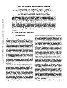
In Fig. S-1 we show the time evolution of the maximum degree kM (t) on the first layer, for different values of β. Notice that kM (t) ∼ (t/s)δ . The effect of the exponent β tuning the width of the delay distribution is evident: the larger the value of β, the closer δ is to 0.5, the value observed in the case of synchronous arrival. Consequently, the rightmost part of the degree distribution is broader when β is close to 1 and becomes more similar to P (k) ∼ k −3 when β increases. Finite size effects

It is interesting to investigate how the properties of the multiplexes generated using the model we propose depend on the number of nodes N . For instance, most of the mean-field predictions for the degree distributions and inter-layer degree correlations are valid in the limit of large N . However, as shown in Fig. S-2 and in Fig. S-3, the properties of the degree distributions and of inter-layer degree-degree correlations are similar to those predicted for large N even for relatively small multiplexes, e.g. with N = 1000. Time complexity

The most efficient algorithm for the construction of a simplex networks based on preferential attachment takes advantage of random sampling with rejection and runs in O(N m2 ). However, in the case of a multiplex the procedure to sample a candidate neighbour j of a newly-arrived node i is a bit more complicated. Let us first consider a two-layer multiplex described by Eq. (S-2). When we sample the candidate neighbours of node i at layer 1 at time t, each node [2] [1] j should be sampled with a probability proportional to akj + (1 − a)kj . The simplest way to implement such P [2] [1] sampling is to construct a vector S whose n-th entry is equal to nj=1 akj + (1 − a)kj (the first element S[0] of the array is set equal to zero); then we sample a real number ζ in the interval (0, S[t]] and we choose the node j such that ζ ≤ S[j] and ζ > S[j − 1]. The construction of the vector S at each time t requires O(t) operations while the sampling of a single node j can be efficiently implemented by binary search, requiring at most O(log(t)) operations per edge, so that the sampling of m edges requires at most O(m log(t)) steps. Thus, the total number of operations needed to sample a layer of a multiplex is: N X

j=m0 +1

O(t) + O(m log(t)) = O(N 2 ) + O(mN log(N )) = O(N 2 + mN log(N ))

(S-49)

It is easy to verify that the construction of a M -layer multiplex requires a number of steps O(M (N 2 + mN log(N ))

(S-50)

which, for m fixed, is dominated by O(M N 2 ). Therefore, the time complexity of this algorithm is linear in the number of layers and quadratic in the number of nodes. We notice that in principle it is possible to construct better algorithms to sample growing multiplexes by implementing a smart policy to update the array S. Randomly-chosen master layer

In the main text we made the simplifying assumption that each node arrives first on the master layer and then on the other layers, after a certain delay. We call this assumption “Equal master layer” (EML). In this Section we briefly comment on the case in which this assumption does not hold, i.e. when a node first arrives either on the first

13

β=1.1 - δ=0.56 β=1.5 - δ=0.53 β=2.0 - δ=0.51 β=2.5 - δ=0.50

1000

kM(t)

100 10000

1e+05

t

FIG. S-1. Effect of β on the maximum degree of a layer. When the exponent β of the delay distribution is close to 1, the maximum degree of a layer scales as (t/s)δ , with δ > 1/2. Consequently, the rightmost side of the degree distribution is broader when β is close to 1 and converges to P (k) ∼ k−3 as β increases.

10

N=1000 N=5000 N=10000 N=50000 N=100000

4

-3

10

~k

0

N(k) 10

-4

0

10

10

1

2

10

3

10

4

10

k FIG. S-2. Degree distribution on the first layer for different values of N . Even for relatively small multiplexes, i.e. N = 1000, the exponent of the degree distribution is almost equal to γ = 3.

or on the second layer, and then arrives on the other layer after a power-law distributed delay. We call this case “Randomly-chosen master layer” (RML), to stress the fact that the master layer of each node is chosen at random among the M layers of the multiplex. In particular, we are interested in the case in which a newly arrived node

14

10000

k(k) N=1000 N=5000 N=10000 N=50000 N=100000 k(k) ~ k

100

1 1

100

10000

k FIG. S-3. Inter-layer degree correlation as a function of N . The shape of the inter-layer degree-degree correlations is already evident even for small values of N . The curves have been vertically displaced to facilitate visual comparison.

selects one of the M layers of the multiples as its master layer with uniform probability p = 1/M . In Fig. S-4, S-5 and S-6 we report, respectively, the degree distributions, the temporal scaling of the degree of the largest hub and the distribution of shortest path lengths and node interdependence for RML with M = 2. The plots suggest that the random choice of the master layer produces a more balanced distribution of super hubs between the two layers, which has a relevant impact on the distribution of shortest path lengths and node interdependence (Fig. S-6). Conversely, the degree distributions and the temporal scaling of the degree of the largest hub are practically indistinguishable from those observed in EML (Fig. S-4 and S-5).

15

10 10

0

a)

-3

P(k) -6

10 0 10 -3

10 10

~k

-3

-6

10 10

0

1

10

100

1000

10

100

1000

b)

-3

P(k) -6

10 0 10 10 10

-3

-6

1

k FIG. S-4. Degree distribution of mixing master layers. The degree distribution of the first layer for the EML (panel a) and the RML (panel b) for β = 1.1 (blue circles) and β = 2.0 (red squares). The random choice of the master layer for each node does not sensibly change the shape of the degree distribution.

16

1000 β=1.1 − δ=0.57 β=1.5 − δ=0.53 β=2.0 − δ=0.52 β=2.5 − δ=0.50 100

kM(t)

10 100

1000

t

10000

FIG. S-5. Temporal scaling of degree for RML. The degree kM of the largest hub in the first layer scales as (t/s)δ , where δ depends on the exponent β of the delay distribution and approaches 0.5 as β increases. Notice that the values of δ are pretty similar to those observed in the case of EML, reportes in Fig. S-1.

17

a) 0.1

P(Li)

P(λi)

0.05

0

2

3

Li

4

5

0.6

λi 0.8

1

b)

0.1

P(Li)

P(λi)

0.05

0

2

3

Li

4

5

0.6

λi 0.8

1

FIG. S-6. Distribution of shortest path lengths and node interdependence for RML. When the master layer of each node is chosen at random, the distribution of shortest path lengths (panel b, left) is more similar to that obtained for synchronous arrival (shaded curve) than that obtained in EML (panel a, left). Conversely, the distribution of node interdependence for RML (panel b, right) sensibly deviates from that obtained for synchronous arrival (shaded curve) and differs from that observed in EML (panel a, right). These results can be explained by a more balanced distribution of super-hubs among the two layers of the multiplex.