Nov 9, 2009 - tributed and multicore masters are contained in a single executable and invoked in the same way. Both All-Pairs and Wavefront are invoked by ...
Journal of Cluster Computing manuscript No. (will be inserted by the editor)
Harnessing Parallelism in Multicore Clusters with the All-Pairs, Wavefront, and Makeflow Abstractions Li Yu · Christopher Moretti · Andrew Thrasher · Scott Emrich · Kenneth Judd · Douglas Thain
November 9, 2009
Abstract Both distributed systems and multicore systems are difficult programming environments. Although the expert programmer may be able to carefully tune these systems to achieve high performance, the nonexpert may struggle. We argue that high level abstractions are an effective way of making parallel computing accessible to the non-expert. An abstraction is a regularly structured framework into which a user may plug in simple sequential programs to create very large parallel programs. By virtue of a regular structure and declarative specification, abstractions may be materialized on distributed, multicore, and distributed multicore systems with robust performance across a wide range of problem sizes. In previous work, we presented the All-Pairs abstraction for computing on distributed systems of single CPUs. In this paper, we extend AllPairs to multicore systems, and introduce the Wavefront and Makeflow abstractions, which represent a number of problems in economics and bioinformatics. We demonstrate good scaling of both abstractions up to 32 cores on one machine and hundreds of cores in a distributed system.
1 Introduction Distributed systems such as clusters, clouds, and grids are very challenging programming environments. (Hereafter, we refer to all of these systems as clusters.) A user that wishes to execute a large workload with some inLi Yu · Christopher Moretti · Andrew Thrasher · Scott Emrich · Douglas Thain Department of Computer Science and Engineering, University of Notre Dame Kenneth Judd Hoover Institution at Stanford University
herent parallelism is confronted with a dizzying array of choices. How should the workload be broken up into jobs? How should the data be distributed to each node? How many nodes should be used? Will the network be a bottleneck? Often, the answers to these questions depend heavily on the properties of the system and workload in use. Changing one parameter, such as the size of a file or the runtime of a job, may require a completely different strategy. Multicore systems present many of the same challenges. The orders of magnitude change, but the questions are similar. How should work be divided among threads? Should we use message passing or shared memory? How many CPUs should be used? Will memory access present a bottleneck? When we consider clusters of multicore computers, then the problems become more complex. We argue that abstractions are an effective way of enabling non-expert users to harness clusters, multicore computers, and clusters of multicore computers. An abstraction is a declarative structure that joins simple data structures and small sequential programs into parallel graphs that can be scaled to very large sizes. Because an abstraction is specialized to a restricted class of workloads, it is possible to create an efficient, robust, scalable, and fault tolerant implementation. In previous work, we introduced the All-Pairs [12] and Classify [13] abstractions, and described how they can be used to solve data intensive problems in the fields of biometrics, bioinformatics, and data mining. Our implementations allow non-experts to harness hundreds of processors on problems that run for hours or days using the Condor [27] distributed batch system. In this paper, we extend the concept of abstractions to multicore computers and clusters of multicore computers. In Section 2, we present the concept of ab-
2
A0
A1
A2
A3
0,4
F
2,4
3,4
Fx
4,4 F1
B0
F
0.5
0.7
0.1
0,3
F
F
3,3
4,3
B1
0.1
1.0
0.3
0.7
0,2
F
F
F
4,2
B2
0.2
0.5
1.0
0.8
0,1
F
F
F
F
D1 Fy Dn
Fj Dm
B3
0.1
0.8
F
1.0
AllPairs( A[i], B[j], F(a,b) )
0,0
1,0
2,0
3,0
4,0
Wavefront( R[x,y], F(x,y,d) )
Ft
Fn
Fk
Makeflow( D[n] )
Fig. 1 Three Examples of Abstractions All-Pairs, Wavefront and Makeflow are examples of abstractions. All-Pairs computes the Cartesian product of two sets A and B using a custom function F. Wavefront computes a two-dimensional recurrence relation using boundary conditions and a custom function F as an input. Makeflow takes an array of dependencies, which could be visualized as a directed acyclic graph structured workload, computes according to the workflow and produces a target file. Using different techniques, each can be executed efficiently on multicore clusters.
stractions, and formally describe All-Pairs, Wavefront and Makeflow. In Section 3, we describe a general architecture for implementing abstractions on multicore clusters. In Section 4, we describe the technical challenges particular to All-Pairs, Wavefront, and Makeflow. In Section 5, we demonstrate weak scaling of each abstractions to large numbers of cores and nodes under controlled conditions. In Section 6, we discuss the advantages of a suite of specific abstractions. In Section 7, we demonstrate applications in bioinformatics and economics robustly running on hundreds of cores in an unreliable distributed system. We conclude with a review of related work and open avenues for research.
2 Abstractions An abstraction is a declarative framework that joins together sequential processes and data structures into a regularly structured parallel graph. An abstraction engine is a particular implementation that materializes that abstraction on a system, whether it be a sequential computer, a multicore computer, or a distributed system. Figure 1 shows three examples of abstractions: All-Pairs, Wavefront and Makeflow. All-Pairs( A[i], B[j], F(x,y) ) returns matrix M where M[i,j] = F(A[i],B[j]) The All-Pairs abstraction computes the Cartesian product of two sets, generating a matrix where each cell M[i,j] contains the output of the function F on objects A[i] and B[j]. This sort of problem is found in many different fields. In bioinformatics, one might compute All-Pairs on a set of gene sequences as the first step of building a phylogenetic tree. In biometrics, one
might compute All-Pairs to determine the accuracy of a matching algorithm on a collection of faces. In data mining applications, one might compute All-Pairs on a set of documents to generate a graph of relationships. Wavefront( R[i,j], F(x,y,d) ) returns matrix R where R[i,j] = F( R[i-1,j], R[i,j-1], R[i-1,j-1] ) The Wavefront abstraction computes a recurrence relationship in two dimensions. Each cell in the output matrix is generated by a function F where the arguments are the values in the cells immediately to the left, below, and diagonally left and below. Once a value has been computed at position (1,1), then values at positions (2,1) and (1,2) may be computed, and so forth, until the entire matrix is complete. The problem can be generalized to an arbitrary number of dimensions. Wavefront represents a number of simulation problems in economics and game theory, where the initial states represent ending states of a game, and the recurrence is used to work backwards in order to discover the effect of decisions at each state. Wavefront also represents the problem of sequence alignment via dynamic programming in genomics. Makeflow( R[n] ) where each rule R[i] is: input files : output files : command returns output files from all R[i] The Makeflow abstraction expresses any arbitrary directed acyclic graph (DAG). Whereas All-Pairs and Wavefront are problems that can be decomposed into thousands or millions of instances of the same function to be run with near-identical requirements, a DAG workload may be structurally heterogeneous and con-
3
sist of programs and files of highly variable runtime and size. Many such problems are found in bioinformatics, where users chain together multiple independent tools to solve a larger problem. Below, we will show Makeflow applied to a genomics problem. On very small problems, these abstractions are easy to implement. For example, a small All-Pairs can be achieved by just iterating over the output matrix. However, many users have very large examples of these problems, which are not easy to implement. For example, a common All-Pairs problem in biometrics compares 4000 images of 1MB to each other using a function that runs for one second, requiring 185 CPU-days of sequential computation. A sample Wavefront problem in economics requires evaluating a 500 by 500 matrix, where each function requires 7 seconds of computation, requiring 22 CPU-days of sequential computation. To solve these problems in reasonable time, we must harness hundreds of CPUs. However, scaling up to hundreds of CPUs forces us to confront these challenges: – Data Bottlenecks. Often, I/O patterns that can be overlooked on one processor may be disastrous in a scalable system. One process loading one gigabyte from a local disk will be measured in seconds. But, hundreds of processes loading a gigabyte from a single disk over a shared network will encounter several different kinds of contention that do not scale linearly. An abstraction must take appropriate steps to carefully manage data transfer within the workload. – Latency vs Concurrency. Dispatching sub-problems to a remote CPU can have a significant cost in a large distributed system. To overcome this cost, the system may increase the granularity of the sub-problems, but this decreases the available concurrency. To tune the system appropriately, the implementation must acquire knowledge of all the relevant factors. – Fault Tolerance. The larger a system becomes, the higher the probability the user will encounter hardware failures, network partitions, adverse policy decisions, or unexpected slowdowns. To run robustly on hundreds of CPUs, our model must accept failures as a normal operating condition. – Ease of Use. Most importantly, each of these problems must be addressed without placing additional burden on the end user. The system must operate robustly on problems ranging across several orders of magnitude by exploring, measuring, and adapting without assistance from the end user. Examples of abstractions beyond the three mentioned above include Bag-of-Tasks [2,24], Bulk Synchronous Parallel [3], and Map-Reduce [4]. None of these models is a universal programming language, but each
is capable of representing a certain class of computations very efficiently. In that sense, programming abstractions are similar to the idea of systolic arrays [11], which are machines specialized for very specific, highly parallel tasks. Abstractions like All-Pairs and Wavefront are obviously than general purpose workflow languages such as DAGMan [27], Pegasus [5], Swift [30], and Dryad [10]. But, precisely because abstractions are regularly structured and less expressive, it is more tractable to provide robust and predictable implementations of large workloads. Once experience has been gained with specific abstractions, future work may evaluate whether more general languages can apply the same techniques.
3 Architecture Figure 2 shows a general strategy for implementing abstractions on distributed multicore systems. The user invokes the abstraction by passing the input data and function to a distributed master. This process examines the size of the input data, the runtime of the function, consults a resource catalog to determine the available machines, and models the expected runtime of the workload in various configurations. After choosing a parallelization strategy, the distributed master submits sub-problems to the local batch system, which dispatches them to available CPUs. Each job consists of a multicore master which examines the executing machine, chooses a parallelization strategy, executes the sub-problem, and returns a partial result to the distributed master. As results are returned, the distributed master may dispatch more jobs and assembles the output into a compact final form. For ease of use and implementation, both the distributed and multicore masters are contained in a single executable and invoked in the same way. Both All-Pairs and Wavefront are invoked by stating directories containing the input data and the name of the executable that implements the function: allpairs function.exe Adir Bdir wavefront function.exe Rdir Without arguments, the distributed master will automatically choose how to partition the problem. When dispatching a sub-problem to a CPU, the distributed master simply invokes the same executable with options to select multicore mode on a given sub-problem, for example: wavefront -M -X 15 -Y 20 -W 5 -H 5 function.exe Rdir
4
4 Evaluate Machine
1. Invoke Abstraction F
Partial Input
3. Dispatch Sub−Problems
Complete Input
Distributed Master
Complete Output 6. Assemble Output
Resource Catalog
Partial Output
Batch System
Multicore Master
Partial Input F
Partial Output
Multicore Master
F 5. Execute Sub−Problems
Multicore Master
F
F
F
F
2. Query and Model System Fig. 2 Distributed Multicore Implementation All-Pairs, Wavefront, and other abstractions can be executed on multicore clusters with a hierarchical technique. The user first invokes the abstraction, stating the input data sets and the desired function. The distributed master process measures the inputs, models the system, and submits sub-jobs to the distributed system. Each sub-job is executed by a multicore master, which dispatches functions, and returns results to the distributed master, which collects them in final form for the user.
Of course, this assumes that the necessary files are available on the executing machine. The distributed master is responsible for setting this up via direct file transfer, or specification through the batch system. Note that this architecture allows for more than two levels of hierarchy – a global master could invoke distributed masters on multiple clusters – but we have not explored this idea yet. The user may specify the function in several different ways. The function is usually a single executable program, in which case the input data is passed through files named on the command line, and the output is written to the standard output. This allows the end user to choose whatever programming language and environment they are most comfortable with, or even use an existing commercial binary. For example, the All-Pairs and Wavefront functions are invoked like this: allpairs_func.exe Aitem Bitem > Output wavefront_func.exe Xitem Yitem Ditem > Output Invoking an external program might have unacceptable overhead if the execution time is relatively short. To overcome this, the user may also compile the function into a threaded shared library with interfaces like this: void * allpairs_function( const void *a, int alength, const void *b, int blength ); void * wavefront_function( const void *x, int xlength, const void *y, int ylength, const void *d, int dlength ); Regardless of how the code is provided, we use the term function in the logical sense: a discrete, self-con-
tained piece of code with no side effects. This property is critical to achieving a robust, usable system. The distributed master relies on its knowledge of the function inputs to provide the necessary data to each node. If the function were to read or write unexpected data, the system would not function. As the results are returned from each multicore master, the distributed master assembles them into a suitable external form. In the case of Wavefront, it is not realistic to leave each output in a separate file (although the batch system may deposit them that way), because the result would be millions of small files. Instead, the distributed master stores the results in an external sparse matrix. This provides efficient storage as well as checkpointing: after a crash, the master reads the matrix and continues where it left off. The distributed master does not depend on the features of any particular batch system, apart from the ability to submit, track, and remove jobs. Our current implementation interfaces with both Condor [27] and Sun Grid Engine (SGE) [8], and expanding to other systems is straightforward. The distributed master also interfaces with a custom distributed system called Work Queue, which we will motivate and describe later. To use Makeflow, a user needs to create a Makeflow script that describes the workflow of his workload. This language is very similar to traditional Make [31]: each rule states a program to run, along with the input files needed and the output files produced. Here is a very simple example: part1 part2: input.data split.py ./split.py input.data out1: part1 mysim.exe ./mysim.exe part1 >out1
5 Table 1 Time to Dispatch a Task
out2: part2 mysim.exe ./mysim.exe part2 >out2 Like All-Pairs and Wavefront, Makeflow can run an entire workload on a local multicore machine, or submit jobs to Condor, SGE, or Work Queue. However, it does not have a hierarchical implementation: only single jobs are dispatched to remote machines. This is because graph partitioning is algorithmically complex, and impractical for heterogeneous workloads where runtime prediction is unreliable. Put simply, Makeflow has greater generality, but this comes at the cost of implementation efficiency, as we will emphasize below.
4 Building Blocks Our overall argument is that highly restricted abstractions are an effective way of constructing very large problems that are easily composed, robustly executed, and highly scalable. To evaluate this argument, we will begin by examining several questions about each abstraction at the level of microbenchmarks, then evaluate the system has a whole.
4.1 Threads and Processes It is often assumed that multicore machines should be programmed via multithreaded libraries or compilers. Our technique instead employs processes, because they are more easily adapted to distributed systems. How does this decision affect performance at the level of a single machine? As a starting point, we constructed simple benchmarks to measure the time to dispatch a null task using various techniques. Each measurement is repeated one thousand times, and the average is shown. (Unless otherwise noted, the benchmark machine is a 1GHz dual core AMD Opteron model 1210 with 2GB RAM running Linux 2.6.9.) Table 1 shows the results. pthread creates and joins a standard POSIX thread on an empty function, fork creates and works for a process which simply calls exit, exec forks and executes an external program, and popen and system create new subprocesses invoked through the shell. It is no surprise that creating a thread is several orders of magnitude faster than creating a process. However, it is not so obvious that popen and system are considerably more expensive than exec, and often vary in cost from user to user. This is because these methods invoke the user’s shell along with their complex startup scripts, which can have unbounded execution time and
Method pthread fork exec popen system
Time 6.3 253 830 2500+ 2500+
µs µs µs µs µs
create troubleshooting problems. If we are careful to avoid these methods, then executing an external program can be made reasonably fast. Moreover, it is only necessary for the execution time to dominate the invocation time: a task in an abstraction running for a second or more is sufficient.
4.2 Concurrency and Data in All-Pairs Of course, within a real program, we must weigh invocation time against more complex issues such as synchronization, caching, and access to data. To explore the boundaries of these issues, we studied the All-Pairs multicore master running in sequential mode on a single machine, comparing 1MB randomly generated files. A simple comparison function counts the number of bytes different in each object. From a systems perspective, this is similar to a biometrics problem, and provides a high ratio of data to computation. Any realistic comparison function would be more CPU intensive, so these tests explore the worst case. In this scenario, we vary several factors. First, we vary the invocation method of the function: create a thread to run an internal function (thread ) or create a process to execute an external program (process). The author of a function is free to choose their own I/O technique, so we also compare buffered I/O byteby-byte (fgetc), block-by-block (fread ), and memorymapped I/O (mmap). A naive implementation would simply iterate over the output matrix in order, causing cache misses at all levels on every access. A more effective method shown in Figure 3 is to choose a smaller block of cells and iterate over those completely before proceeding to the next block. The width of the block is called the block size. (This technique is sufficient for our purposes, but see Frigo et al [7] for more clever methods.) Figure 4 shows the relative weight of all these issues. Each curve shows the runtime of a 1000×10 comparison over various block sizes. The two slowest curves are thread and process, both using fgetc. The two middle curves are process using fread and mmap, and the fastest is thread with mmap. All curves show significant slowdown when the block size exceeds physical memory.
6
...
Linear Method
Turnaround Time (s)
100000
...
m
... ... ... ... ... ... ...
n
... ... ...
... ... ...
... Blocked Method ... ... ... ...
... ... ...
10000 Dispatch Latency 30s 10s 1s 0s
1000 1
Fig. 3 Linear Method vs Blocked Method. The linear method evaluates cells in the matrix line by line. The blocked method evaluates cells block by block with a width chosen to fit in the file system buffer cache.
Elapsed Time (seconds)
1800
4
8
16
32
Block Size
Fig. 6 The Effect of Latency on Wavefront The modeled runtime of a 1000×1000 Wavefront where each function takes one second to complete, with varying block size and dispatch latency. As dispatch time increases, the system must increase block size to overcome the idle time.
1600 1400 1200 1000 800 600
process - fgetc thread - fgetc process - fread process - mmap thread - mmap
400 200 0 0
1
2
Block Width (Multiple of RAM)
Fig. 4 Threads, Processes, and I/O Techniques. The performance of a data intensive 1000×10 All-Pairs in sequential mode using threads and processes with various I/O techniques. While threads provide the best performance, processes are a reasonable method even on this worst case. 100000 Elapsed Time (seconds)
2
Two Sub Problems Single Core Dual Core
10000
1000 0
1
2
Block Width (Multiple of RAM)
Fig. 5 Multicore vs Sub-Problems. The performance of an 1000×10 All-Pairs in sequential mode, in dual-core mode, and as two independent sequential sub-problems, using various block sizes. This demonstrates the importance of an explicit multicore strategy.
Clearly, threads with mmap execute twice as fast as the next best configuration. If the user is willing to write a thread-safe function for use with the abstraction, they should do so. However, the use of processes is only twice as slow in this artificial worst case and will not fare as poorly with a more CPU-intensive function. Moreover, the appropriate use of virtual memory by the abstraction and the I/O technique chosen by the function are much more significant factors than the difference between threads and processes. We conclude that using processes to exploit parallelism is a reasonable tradeoff if it improves the usability of the system. (We re-emphasize that each abstraction can accept either an external program or a threaded internal function. So far, none of our users has chosen to use threads.) Next we consider how to carry out All-Pairs on a multicore machine. Although there are many possible ways, we may consider two basic strategies. One is to generate N contiguous sub-problems, and allow each core to run independently. The other is to write an explicit multicore master that proceeds through the entire problem coherently, dispatching individual functions to each core. Figure 5 compares both of these against a simple sequential approach. As can be seen, the subproblem approach performs far worse, because it does not coordinate access to data, and caches at all levels are quickly overwhelmed. Thus, we have shown it is necessary to have a deliberate multicore implementation, rather than treating each core as a separate node.
4.3 Control Flow in Wavefront As we have shown, the primary problem in efficient AllPairs is managing data access. However, in Wavefront the problem is almost entirely control flow. The first task of the problem is sequential. Once completed, two
7 120 Tasks Running
100
With Fast Abort
80 60 40
Without Fast Abort
20 0 100 200 300 400 500 600 700 800 900 1000 Elapsed Time (seconds)
Fig. 7 The Effect of Fast Abort on Wavefront The startup behavior of a 500×500 Wavefront with and without Fast Abort. Without Fast Abort, every delayed result impedes the increase in parallelism, which stabilizes around 20. With Fast Abort, delays are avoided and parallelism increases steadily.
tasks may run in parallel, then three, and so forth. If there is any delay in dispatching or completing a task, this will have a cascading effect on dependent adjacent tasks. We will consider two control flow problems: dispatch latency and run-time variance. Figure 6 models the effect of latency on a Wavefront problem. This simple model assumes a 1000×1000 problem where each task takes one second to complete. On the X axis, block size indicates the size of sub problem dispatched to a processor. Each curve shows the runtime achieved for a system with dispatch latency ranging from zero (e.g. a multicore machine) to 30 seconds (e.g. a wide area computing grid). As block size increases, the sub-problem runtime increases relative to the dispatch latency, but less parallelism is available because the distributed master must wait for an entire sub-problem to complete before dispatching its neighbors. The result is that for very high dispatch times, a modest block size improves performance, but cannot compete with a system that has lower dispatch latency. So, the key to the problem is to minimize dispatch latency. Although Wavefront can submit jobs to Condor and SGE batch systems directly, the dispatch latency of these systems when idle is anywhere from ten to sixty seconds, depending on the local configuration. For shortrunning functions, this will not result in acceptable performance, even if we choose a large block size. (This is not an implementation error in either system, rather it is a natural result of the need to service many different users within complex policy constraints.) To address this, we borrowed the idea of a fast dispatch execution system as in Falkon [17]. We built a simple system called Work Queue that uses lightweight worker processes that can be submitted to a batch system. Each contacts the distributed master, and provides
Fig. 8 Asynchronous Progress in Wavefront A progress display from a Wavefront problem. Each cell shows the current state of a portion of the computation: the darkest gray in the lower left corner indicates incomplete, the lighter gray in the upper right indicates complete, and the light cells in between are currently running. The irregular progress is due to heterogeneity and asynchrony in the system.
the ability to upload and execute files. This allows for task dispatch times measured in milliseconds instead of seconds. Workers may be added or removed from the system at any time, and the master will compensate by assigning new tasks, or reassigning failed tasks. However, even if we solve the problem of fixed dispatch latency, we must still deal with the unexpected delays that occur in distributed systems. When Work Queue runs on a Condor pool, a running task may still be arbitrarily delayed in execution. It may be evicted by system policy, stalled due to competition for local resources, or simply caught on a very slow machine. To address these problems, the Work Queue scheduler keeps statistics on the average execution time of successful jobs and the success rate of individual workers. It makes assignments preferentially to machines with the fastest history, and proactively aborts and re-assigns tasks that have run longer than three standard deviations past the average. These techniques are collectively called Fast Abort. Figure 7 shows the impact of Fast Abort on starting up a 1000×1000 Wavefront on 180 CPUs. Without Fast Abort, stuck jobs cause the workload to however around twenty tasks running at once. With Fast Abort, the stragglers are systematically resolved and the concurrency increases linearly until all CPUs are in use. Figure 8 shows this behavior from another perspective. The distributed master periodically produces a bitmap showing the progress of the run. Colors indicate the state of each cell: red is incomplete, green is running, and blue is complete. Due to the heterogeneity of the underlying machines, the wave proceeds irregularly. Although an N×N problem should use N CPUs at maximum, this perfect diagonal is rarely seen.
8
5 Putting it All Together
4500 4000
Time (second)
3500 3000 2500 2000 1500
cluster multicore
1000 500 0 0
5
10
15
20
25
Number of Cores
Fig. 9 Makeflow on Multicore and Cluster The performance of a genomics application run through Makeflow, using 1-24 cores on both a multicore machine and a cluster using Work Queue.
4.4 Greater Generality with Makeflow Makeflow provides a different type of building block for large multicore workflows with abstractions. Makeflow combines many functions together (instead of many instances of the same function) to express more complex series of operations. Makeflow uses a syntax very similar to traditional Make, but it differs in one critical way: each rule of a Makeflow must exactly state all of the files consumed or created by the rule. (In traditional Make, one can often omit files, or add dummy rules as needed to affect the control flow.) Makeflow is more strict, but this allows it to accurately generate batch jobs, exploit common patterns of work, and schedule jobs to where their data is located. This allows Makeflow to run correctly on both local multicore machines as well as a distributed system. The Makeflow abstraction can be configured to use different numbers of cores. Figure 9 shows the turnaround times varying the number of cores used with two different options for executing a genomics workload on 1-24 cores. The top curve (“cluster”) presents Makeflow using Work Queue, with workers submitted to remote machines as Condor jobs. The bottom curve (“multicore”) executes all work as Makeflow-controlled local processes, in which Makeflow automatically takes advantage of multiple cores on the submitting machine. Makeflow jobs running locally outperform jobs tasked to remote workers and scale well up to the number of available cores.
In a well-defined dedicated environment in which the distributed master knows exactly which resources will be used, a model can partition work to the resources in such a way as to optimize the workload [28]. This applies to multicore environments as well – the distributed master could build multicore assumptions into the model to optimize a workload. However, this finelytuned partitioning does not adapt well to heterogeneous environments or resource unavailability. Previous work derived a more realistic solution for modeling the turnaround time of an All-Pairs workload in a cluster [12]. Is it possible to use the multicore version of the All-Pairs abstraction transparently beneath the cluster abstraction? If the abstraction is to use the multicore master transparently, then it must continue to exclude considerations of the number of cores per node from the model . If the workload is benchmarked on a single-core system or with a single-threaded executor, then the model will choose appropriate resources to run the workload efficiently assuming single-threaded operation. Adding multicore execution to this workload, then, will only serve to make the batch jobs complete faster on the multicore resources. It does not change the overall workload any more than having benchmarked on a slow node would: the success of the model in avoiding disastrous cases is maintained, the faster resources (in this case multicore nodes) will account for a greater portion of the batch jobs than their “fair share”, and any long-tail from slow nodes would extend out at most to the same duration as without any multicore nodes. So it is possible, but this is little solace if there is a clearly better solution for modeling a distributed AllPairs workload using multicore resources. Another option is to integrate the multicore master (instead of the original single-threaded executor) into the benchmarking process for the model. If the function runtime is benchmarked using the multicore master, then the function execution time (computed as the average time per function over a small set of executions) will be comparable to the expected execution of batch jobs on the same number of cores. This is a good approach for submitting to homogeneous clusters of resources in which the same number of cores are available for every batch job. In a heterogeneous environment, however, this only serves to exacerbate the model’s assumption that the benchmark node reflects the cluster’s resources. Whereas the original model conceded that individual resources might be perhaps a generation newer (faster) or older (slower) than the benchmark node, the inclusion of multicore uncertainty into the benchmarking increases the poten-
4500 4000 3500 3000 2500 2000 1500 1000 500 0
16000
8-Core Real 8-Core Model
Runtime (seconds)
Runtime (seconds)
9
64-Core Cluster Real 64-Core Cluster Model
14000 12000 10000 8000 6000 4000 2000 0
0
100 200 300 400 500 600 700 800 900 1000
0
500 1000 1500 2000 2500 3000 3500 4000
Problem Size
Problem Size
Fig. 10 Accuracy of the All-Pairs Model on Multicore and Cluster The real and modeled performance of an All-Pairs benchmark of varying sizes on a 8-core machine (left) and an 64-core cluster (right). 12000
32-Core Real 32-Core Model
35000
Runtime (seconds)
Runtime (seconds)
40000 30000 25000 20000 15000 10000 5000
180-Core Cluster Real 180-Core Cluster Model
10000 8000 6000 4000 2000
0
0 0
50 100 150 200 250 300 350 400 450 500
0
50 100 150 200 250 300 350 400 450 500
Problem Size
Problem Size
Fig. 11 Accuracy of the Wavefront Model on Multicore and Cluster The real and modeled performance of a Wavefront benchmark of varying sizes on a 32-core machine (left) and an 180-core cluster (right).
Time (second)
50
60
24-Core Real 24-Core Model
50 Time (second)
60
40 30 20 10
60-Core Cluster Real 60-Core Cluster Model
40 30 20 10
0
0 50
100
150
200
250
Size (unit of workload)
50
100
150
200
250
Size (unit of workload)
Fig. 12 Accuracy of the Makeflow Model on Multicore and Cluster The real and modeled performance of a Makeflow benchmark of varying sizes on a 24-core machine(left) and a 60-core cluster(right).
tial range of resource capabilities and thus the potential for long-tail effects in a workload. Another option would be to include a coefficient of the average number of cores within the model. Because the model includes a component for the time to complete a single batch job, an adjustment for the number of cores could be made by dividing the the batch job execution time in the model by this average. This retains the same prerequisite measurements (plus the calcula-
tion of the average number of cores), however it has several limitations. First, the pool of resources must be well-defined so that the average number of cores may be determined; but because the model is used to select the appropriate number of resources, the exact set of hosts is not known a priori. Thus, the average number of cores available for each host is a pool average rather than one specific to the actual resources used. Further, contention for resources means that not all hosts will
10 5000 Runtime (seconds)
Runtime (seconds)
500 400 300 200 Automatic Cluster Model Local Model
100 0 0
100
200
300
400
4000 3000 2000 Automatic Cluster Model Local Model
1000 0
500
0
50
Problem Size
100
150
200
250
300
Problem Size
Fig. 13 Selecting An Implementation Based on the Model These graphs overlay the modeled multicore and cluster performance on problems of various sizes for All-Pairs (left) and Wavefront (right). The dots indicate actual performance for the selected problem size. As can be seen, the modeled performance is not perfect, but it is sufficient to choose the right implementation.
6 Why Multiple Abstractions? With the Makeflow abstraction for arbitrary DAG workflows, could we choose to use it as a general tool instead of implementations of the specific abstractions mentioned above? In our experience, the answer is that we could, but in doing so we lose many of the problemspecific advantages given by the less general abstractions. We carry out All-Pairs on a 24-core machine using
100000 10000 Time (second)
be utilized equally or predictably, which presents the same problem in trying to include a factor of the number of cores in the turnaround time model. This is especially problematic as we move beyond workstations with at most a few cores: unavailability of a machine with dozens of cores significantly changes the average number of cores of the available machines. With that said, can we accurately model the performance of our abstractions? Figure 10 shows the modeled performance of All-Pairs workloads of varying sizes running on an 8-core machine and a 64-core cluster. Figure 11 shows the modeled performance of Wavefront workloads running on a 32-core machine and a 180-core cluster. In both cases, the multicore model is highly accurate, due to a lack of competing users and other complications of distributed systems. Both models are sufficiently accurate that we may use them to choose the appropriate implementation at runtime based on the properties given to the abstraction. Figure 12 shows the modeled performance of Makeflow workloads running on a 24-core machine and a 60-core cluster. Figure 13 compares the multicore and cluster models for the previous All-Pairs and Wavefront examples, and demonstrates the actual performance achieved when selecting the implementation at runtime.
1000 100 10 1
Makeflow Allpairs
0.1 0.01 0
200
400
600
800
1000
Size (width)
Fig. 14 Solving All-Pairs with Makeflow and All-Pairs This figure shows the time to complete an All-Pairs problem of various sizes using the general Makeflow tool and the specific AllPairs tool. The more general tool is considerably more expensive, because it uses files for output storage, and is unable to dispatch sub-problems to multicore processors.
both the all-pairs multicore abstraction and the Makeflow abstraction. We vary the size of the workloads from creating a 10×10 matrix to creating a 1000×1000 matrix. Each matrix cell is computed by comparing two 20KB files. With the Makeflow abstraction, each cell value depends on a comparison and the cell value is stored in a file after it is computed. And we have to write an additional program, which depends on all the cell value files, to extract all cell values from generated files and put them into the target matrix. The running time of both abstractions on different workloads are shown in Figure 14. It is easy to see that the All-Pairs multicore abstraction scales almost linearly as the workload increases. However, the Makeflow abstraction is several orders of magnitude slower at this problem, because it
11
uses files for output storage, and is unable to manage work in organized blocks. The increased generality of Makeflow has a significant price, so we conclude that there is a great benefit to retaining specific abstractions such as All-Pairs and Wavefront for specialized problems.
7 Applications
90 80 70 60 50 40 30 20 10 0 0
In a previous paper [12], we demonstrated a number of applications of All-Pairs, so here we will focus on applications of Wavefront and Makeflow. Our example applications run on an open Condor pool of approximately 600 CPUs, consisting of heterogeneous desktop machines, homogeneous research clusters, and multicore servers ranging from 4-32 CPUs. Clock speeds range from 500MHz to 4GHz. The number of CPUs changes unpredictably as desktop users come and go, and other workloads enter and leave the system. Thus, these results show that our system achieves reasonable performance under adverse conditions on real applications. We use the term speedup with the usual definition: sequential runtime divided by actual runtime. However, note that the maximum possible speedup is not the number of processors. Consider an idealized machine with P processors running an N ×N problem with P ≥N . In the first timestep, one task will run, then two, and so forth, until the diagonal is reached in N steps. Then, N − 1 tasks run simultaneously and so on down to one task, giving a parallel runtime of (2N − 1) timesteps. The sequential runtime is N 2 , so the best possible speedup is N 2 /(2N − 1) or N/2. But, if P