Aug 2, 2011 - FIR filters are vastly used in multi-mode systems where the behavior of the .... Using Xilinx FPGAs the rest of the system that is not being reconfigured ...... We generated these filters in Matlab using Signal processing toolbox. The ..... [22] Xilinx Core Generator System, http://www.xilinx.com/tools/coregen.htm.
Center for Embedded Computer Systems University of California, Irvine ____________________________________________________
Heterogeneous Mapping to Minimize Resource Usage under Maximal Spatial Reuse Constraints for FIR-like Structures Amir Hossein Gholamipour, Michael Dillencourt, Fadi Kurdahi and Ahmed Eltawil Center for Embedded Computer Systems University of California, Irvine Irvine, CA 92697-2620, USA
{ amirgh, dillenco, kurdahi, aeltawil }@uci.edu CECS Technical Report 11-01 August 2nd, 2011
Abstract FIR filters are vastly used in multi-mode systems where the behavior of the system changes based on user inputs or changes in the operational environment. FIR filters used for each mode of operation have different sets of parameters (coefficient sets). Partially reconfigurable FPGA platforms are shown to be viable choices to implement multi-mode filters. Joint optimization of the filters generates filters with common modules to reduce reconfiguration overhead. At physical design level, these common modules should be mapped to physical locations on the chip called Partially Reconfigurable Regions (PRRs). Furthermore depending on the availability of DSP blocks, we can implement some of these modules using DSP blocks. In this work we study the problem of reconfigurable module mapping to minimize the reconfigurable area of the filter while fully exploiting module reuse and available DSP blocks. We show that the decision problem is NPcomplete and propose an ILP formulation and a heuristic to reduce the area. Our experiments show that the quality of the results of our heuristic is within 1% of the optimal result. Furthermore the results show the importance of area minimization to reduce the overall reconfiguration overhead.
ii
1 Introduction An increasing number of digital systems, from wireless devices to multi-media terminals, are characterized by their multi-mode operation. This refers to the ability of a system to modify its characteristics or behavior based on user inputs or changes in the operational environment. For example, in a WiMax terminal, the characteristics of the MAC and PHY can be changed based on the current status of the wireless channel. In spectrum sensing, the matched-filter used to find idle frequency bands is changing periodically to accommodate the characteristics of the protocols operating in the corresponding band. Finally, in pattern matching applications, the pattern being searched can be modified by changing the dimensions and coefficient values of an image template. Multi-mode systems vastly incorporate Finite Impulse Response (FIR) filters as one of the main components in their design. This is due to FIR filters’ inherent stability and linear phase. Therefore, one of the challenges of designing multi-mode systems is to design multi-mode FIR filters where the characteristics of the filter (value and number of coefficients) are changing depending on the mode of operation. Due to large data rate processing demand of applications incorporating multi-mode filters, software-programmable processors are not viable options to implement a multimode filter. ASICs on the other hand lack the flexibility to conform to varying characteristics of the design. FPGAs provide a third alternative for implementing multimode filters. Their short design cycles and reconfiguarbility give them an advantage over ASICs, their inherent parallelism can be used to support high data rates, and they can be easily customized to support irregular datapaths with variable bit widths. Furthermore
1
support for dynamic partial reconfiguration (DPR) in Xilinx FPGAs also enables the modification of a system's architecture by loading or swapping logic blocks in userdefined reconfigurable regions while the FPGA device is operational. The structure of an n-tap FIR filter consists of n coefficients and is shown in Figure 1. The Z-1 boxes represent delay elements. X(n)
Z-1
C1
X(n-1)
X(2)
Z-1
Cn-1
C2
Z-1
X(1)
Z-1
Cn
Level 0 (L0) Level log n (Llog(n))
Figure 1. Direct-form structure of an n-tap FIR filter
The filter structure shown in Figure 1 can be optimized based on the value of the coefficients. However since the reconfiguration overhead is non-negligible, in our previous work in [23] we proposed to split the filter structure in two sections: A section which is static across all filters and a reconfigurable section which is optimized for each coefficient set. To identify the two sections, we split the filter at an arbitrary level of structure as shown in Figure 1. Level 0 (L0) is to split the structure after the multiplier block of the filter. Each additional level contains one level of resources (adders of the adder tree). With this approach we can manage the reconfiguration overhead by choosing the level at which we split the structure. To reduce the size and reconfiguration overhead of a filter we need to optimize the reconfigurable section of each filter. In [23], we introduced Joint Filter Design (JFD) problem which is the problem of designing a reconfigurable filter structure for a given 2
sequence of filters. We proposed to jointly optimize the filter structures to reduce reconfiguration overhead. The idea is to exploit similarity of the filters characteristics, to design modules that are shared across the filters in the sequence of reconfiguration. However while increasing the number of shared modules across designs could potentially reduce reconfiguration overhead, the end result is widely dependent on the efficiency of physical design of the filter. In this work we follow Module-based partial reconfiguration scheme introduced in [1] and [2]. In this scheme the modules of the design are categorized as static modules and reconfigurable modules. Our description of static and reconfigurable sections of a filter fits this definition. Static modules are not reconfigured during the run-time of the system while reconfigurable modules are reconfigured at run-time. As we will explain later in this work following partial reconfiguration design flow mandates identifying sets of reconfigurable blocks that should be mapped to the same physical region on the chip. This mapping as part of the design process has non-negligible impact on area and reconfiguration overhead of the design. To overcome the limitations of the physical design level, in this work we propose an additional step called mapping. This step precedes floorplanning in the design flow. We formally define mapping problem and theoretically analyze it. We subsequently propose solutions to this problem. The rest of this paper is as follows: Section 2 briefly explains partial reconfiguration design flow and the limitations it imposes on the design and design flow. Section 3 explains the related work. Section 4 defines PRM2PRR mapping and theoretically analyzes it. We furthermore propose solutions to PRM2PRR mapping problem in this section. Section 5 studies the problem of partial filter implementation using DSP blocks embedded on
3
FPGAs. In this section after motivating and defining a problem we theoretically analyze the problem and propose a solution to it. Finally in Section 6 we present the result of our experiments and then we conclude.
2 Partial Reconfiguration Design Flow There are two approaches to partial reconfiguration. These two approaches in Xilinx terminology are “Difference-based” and “Module-based” partial reconfiguration. Difference-based partial reconfiguration is meant to be used for making small changes in the logic implemented on the FPGA. This is mainly done using FPGA editor where a designer can change the logic function implemented using LUTs. Subsequently a partial bit-stream is generated to reconfigure that portion of the design. Using this approach we can slightly change the circuit implemented on the FPGA, however for most of practical applications this remains unrealistically limited. In module-based partial reconfiguration on the other hand, as the name suggests, reconfiguration is implemented at module-level. This means that the whole modules are replaced by other modules while reconfiguring the design. Using Xilinx FPGAs the rest of the system that is not being reconfigured continues execution during reconfiguration. As mentioned in [2] there are 7 phases involved in designing and implementing a partially reconfigurable circuit on FPGA. The first two phases are directly related to the focus of this work while the rest are mostly implementation related and specific to toolsets, therefore we do not discuss those phases. Interested readers can refer to [2] for more details on partial reconfiguration implementation.
4
2.1 Planning and Synthesis The designer begins by identifying the opportunity to deploy dynamic reconfiguration. He/she partitions the design into a static subset and one or more dynamic (reconfigurable) subsets. As mentioned earlier in this section, the static modules in the design remain the same during the course of reconfiguration while the reconfigurable modules are being reconfigured. In this methodology, the term Partially Reconfigurable Region (PRR) is used to describe the area of the FPGA that will be reserved for implementing a dynamically reconfigurable module. The term Partially Reconfigurable Module (PRM) is used to describe the implementation of a single dynamic module that will be mapped into a PRR. Each task in the subset will be implemented as a partially reconfigurable module (PRM) that will be swapped in and out of its corresponding PRR at run-time. The designer should furthermore establish the nature of communication between modules. The interconnection among reconfigurable modules and between reconfigurable modules and static modules is possible through specific connections called “Bus Macros”. The designer should organize the HDL source files for reconfigurable and static modules in a pre-determined file structure. The details on how to organize the HDL source files are explained in [2] and thus is omitted from this thesis.
2.2 Mapping and Budgeting The goal of the mapping and budgeting phase is to determine the size and location of the PRRs and to lock down the placement of the bus macros. This is done by determining the PRMs for each design that are “mapped” to PRRs. PRMs that are mapped to the same PRR do not coexist at the same time on the chip i.e they replace each other in the course of reconfiguration. The PRRs in a design are restricted according to the PRMs that are 5
mapped to them. The interface of the PRRs should be so that it represents the interface of all the PRMs that are mapped to it. Furthermore the area and shape of PRRs should embody all the PRMs that are mapped to it. This means that a PRR is at least as large as the largest PRM mapped to it. The most important design factors which are power, performance, area and reconfiguration overhead are directly affected by the quality of mapping phase. The impact of mapping on the area of a design is shown through an example later in this chapter. Mapping phase also directly and indirectly affects power consumption of the system. This is because static power consumption is directly related to the area of the design. A smaller design consumes lower static power. Also as it was shown in prior research publications as two examples in [12] and [5], that partial reconfiguration incurs non-negligible power consumption overhead. Thus reducing the amount of reconfiguration also affects total power consumption of the system. The impact of mapping on performance is also two-folds. On one hand it affects the reconfiguration overhead which defines the speed at which we can reconfigure one design to implement the next. On the other hand it affects the clock speed and timing within individual designs. Prior work in this area has shown the impact of mapping on wire-length which is directly related to clock speed. For example in [4] and [11] the authors studied multiple possible mapping (the authors use the term “matching”. In this subsection we use “mapping” and “matching” interchangeably) across PRMs in two different designs and showed that different matching sets results in varied timing across individual designs. As well they showed that a proper matching effectively reduces reconfiguration overhead across designs. In [11] the authors proposed a simulated
6
annealing move to change the matching across possible floorplan solutions to find the best matching while floorplanning the designs. In this work after reviewing the related work in Section 3, in Section 4 we study PRM2PRR mapping problem and theoretically analyze the complexity of the problem. We will show that mapping is an NP-hard problem. Therefore we propose an ILP-based exact solution to the problem as well as a heuristic to give an acceptable solution in polynomial time.
3 Related Work Placement-aware partial reconfiguration is not a new subject of study. In early works on partial reconfiguration in [5] the authors proposed to match two successive circuit configurations to locate the common components between them. They proposed a weighted bipartite graph representation of the two configurations and run matching to determine the common components. At floorplan level the authors in [4] and [11] studied the effect of component reuse on the quality of physical design for reconfigurable design implementation. In specific they studied the problem of matching to match common components across designs in the sequence of reconfiguration. As an example, assume that design 1 has 4 multipliers while design 2 which will be reconfigured after design 1 has 5 multipliers. The authors in [4] and [11] showed that, the decision to choose which multipliers to match affects the wire-length for the individual designs which in turn affects the clock speed at which the designs are running. Furthermore, the result of their study shows that to avoid routing congestion it may be beneficial to place a shared module at another location on FPGA which incurs extra reconfiguration overhead. The 7
model of reconfiguration in their work can be best described by difference-based partial reconfiguration which incurs different constraints than that of module-based partial reconfiguration flow. To find an efficient placement, they proposed specific moves in their simulated annealing-based floorplanner to modify the mapping of shared modules. In [13] the authors proposed a unified communication infrastructure for several PRMs in a system to communicate. The sizes of PRRs were assumed to be fixed and the authors proposed a simulated annealing-based solution to map PRMs to PRRs to exploit reuse. The platform introduced in this work is close to the platform that is naturally created in our joint-filter design approach. Therefore this work is close to what we are proposing. However this work greatly lacks formal theoretical study of the problem which brings up opportunities to study other optimization problems that will be discussed in mapping. Other works including [14] and [15] studied reconfiguration speedup using module relocation on the FPGA. Relocation makes it possible to use the bitstream on a section of FPGA to configure another section of the FPGA. While this is much faster than transferring the bitstream from off-chip memory it still needs to read configuration bitstream from one location on the chip and modify and write the bitstream on another location. Compared to the previous work in this area, we are introducing a problem that is necessary to solve as part of partial reconfiguration design flow. However because of the characteristic of filter design problem that we are proposing in this thesis, the problem to solve is simpler than the general case. In general mapping, one should consider the interface of the PRMs while mapping them to PRRs. This is usually assumed to be the designer’s job to make PRMs that have similar interfaces and map them to PRRs. In the
8
case of filter design problem, the interfaces of PRMs are indeed the same. However to propose an automated solution to solve mapping for all designs, the tool should be able to create a unified interface across PRMs that are mapped to the same PRR. While this is somewhat challenging, the main challenge comes from the fact that wire-length cannot be ignored in mapping anymore. In our approach proposed here, since the interconnection among Static modules and all the PRMs is the same, the problem with wire-length is not significant. Thus we propose our solution just to optimize the area of the PRRs or to optimize total reconfiguration overhead. As we will explain, just considering these two factors the problem is already intractable. Therefore adding wire-length just increases the complexity of the problem which should be studied as part of the future work to this thesis.
4 PRM2PRR Mapping As mentioned in Section 2 we need to identify a mapping of PRMs to PRRs before floorplanning, placement and routing of the designs. The example shown in Figure 2 clarifies the impact of mapping on area of reconfiguring designs. In Figure 2.a and Figure 2.b the floorplanning for individual designs D1 and D2 is shown. The modules shown in the figure represent PRMs for designs D1 and D2.
9
FPGA
FPGA C22
C11
C12
C21 D1
D2
(a)
(b)
Mapping 1
Mapping 2
C12 and C21 → C2 C11 and C22 → C1
C12 and C22 → C3 C11 and C21 → C4
FPGA
FPGA C3
C1 C2
C4
AC1= max( AC12, AC21)
AC3= max( AC12, AC22)
AC2= max(AC11, AC22)
AC4= max(AC11, AC21)
Area = AC1 + AC2
Area = AC3 + AC4
Reconf. Overhead = AC1 + AC2
Reconf. Overhead = AC3 + AC4 (d)
(c)
Figure 2. Block mapping for a partially reconfigurable system and its impact on area
In Figure 2.c PRMs C12 of design D1 and C21 of design D2 are mapped to PRR C2. As well PRMs C11 and C22 are mapped to PRR C1. For the reconfigurable system shown in Figure 2.c the total area of the design are equal to the cumulative area of C1 and C2. However by mapping PRMs C12 and C22 to the same PRR C3 in Figure 2.d and PRMs C11 and C21 to PRR C4, we could reduce the area to the cumulative area of C3 and C4. From Figure 2 it is clear that Mapping 2 (in Figure 2.d) results in smaller area than Mapping 1 (in Figure 2.c), furthermore as the reconfiguration overhead is equal to the total area that 10
is being reconfigured, by reducing the area we are also indirectly reducing the reconfiguration overhead. Mapping phase can also directly affect reconfiguration overhead. Figure 3 shows the physical layout of a filter structure on an FPGA chip. It also shows the reconfigurable and static sections of a reconfigurable filter. As shown the reconfigurable modules and the static module are connected through “bus macros” as described in Section 2.
Reconfigurable PRMn,1 PRR1
PRRn
Bus macro
PRMn,2
PRMn,k
Static Figure 3. Reconfigurable filter implementation on FPGA
PRMn,1, PRMn,2, …, PRMn,k in Figure 3, are modules that are generated for filters F1, F2, …, Fk as the result of applying JFD. We can further assume that some of these PRMs e.g PRMn,i and PRMn,i+1 are the same i.e they are shared across filters Fi and Fi+1. In this example all these modules are mapped to the same PRRn. The area of PRRn should be at least as large as the largest PRM assigned to it. On the other hand, we can only avoid reconfiguring common modules across filter designs, if they are mapped to the same PRR. As an example we can only avoid reconfiguring PRMn,i while reconfiguring from Fi
11
to Fi+1 when both PRMn,i and PRMn,i+1 are mapped to the same PRRn. Mapping shared PRMs to different PRRs, results in additional reconfiguration overhead while the area of the filter may stay the same. Thus it is important to augment the JFD approach with an efficient mapping to exploit the opportunity of having shared modules across designs. Mapping phase in the design process can be optimized for different objectives, including minimizing area, minimizing reconfiguration overhead, etc. The objective of PRM2PRR mapping in this thesis is to minimize total area of the design under the constraint that all the shared modules should be mapped to the same PRR to reduce reconfiguration overhead. To solve the mapping problem, we model the PRMs of each filter design and the PRRs as shown in Figure 4. In Figure 4, the PRMs of each of the filters F1, F2, F3 and F4 are laid out vertically i.e P1, P2, P3 and P4 belong to filter F1, etc. The PRMs that are connected across different columns are the ones that are shared across two or more designs. There are two numbers associated with each PRM as shown in Figure 4. The number shown on top is the area of the PRM and the number shown at the bottom determines the number of filter taps implemented in this PRM. As an example, size of P1 is 45 (slices) and it implements 15 taps of filter F1. For filters with less number of PRMs (e.g F2) we insert PRMs of size 0 (PRM P11). We map all the PRMs on the same row to one PRR. Therefore the PRMs that are shared among multiple designs are not mapped to the same PRR if they are not placed on the same row.
12
F1
F2
F3
45 15 P1
33 17 P5
33 17 P5
38 25 P8
PRR1
25 15 P2
25 15 P2
45 15 P6
45 15 P6
PRR2
20 11 P3
0 0
P11
40 15 P7
28 10 P9
PRR3
15 5 P4
15 5 P4
15 5 P4
25 12 P10
PRR4
F4
PRR Size 45
40
33
25
Figure 4. Mapping clusters (PRMs) to PRRs
Theorem 1: Lower bound for implementation area is achieved by sorting the PRMs of each design based on their sizes (see Figure 5). Proof: We prove Theorem 1 by way of contradiction. We assume that there is a mapping which results in area smaller than what is proposed in Theorem 1 and shown in Figure 5. Without loss of generality we assume that the areas of PRMs of each filter are distinct. We assume that by placing the PRMs based on Theorem 1, the area of PRR1 is equal to PRM P1, the area for PRR2 is equal to PRM P2, etc. We assume there are a total of m PRRs. We define 𝐴𝑃1 to be the area for PRM P1. We can safely assume that 𝐴𝑃1 > 𝐴𝑃2 >
⋯ > 𝐴𝑃𝑚 . For mapping M1, the area cost of mapping is equal to 𝑀1 = 𝐴𝑃1 + 𝐴𝑃2 + ⋯ +
𝐴𝑃𝑚 . We assume that there is another mapping M2 with total area smaller than M1. Since
the area of PRMs are distinct we can conclude that in M2 the set of PRMs P1, P2, …, Pm are mapped to k different PRRs where k < m. Thus two PRMs, Px and Py ( x < y ) are
mapped to the same PRR (pigeonhole principle). In mapping M1, there is another PRM Pt on the same design as Py that is mapped to the same PRR as Px. Since the assumption in
13
M1 is that we need to sort the PRMs in each design first, then we can assume that 𝐴𝑃𝑡 > 𝐴𝑃𝑦 . At the same time since the size of the PRMs are distinct and that the area of
PRRx is equal to Px, then we conclude that 𝐴𝑃𝑥 > 𝐴𝑃𝑡 . Exchanging Py and Pt in mapping
M2 considering that inequalities mentioned above either reduces the area or does not affect it. We can continue this analysis for all Pi ( 1 ≤ 𝑖 ≤ m ) that are mapped to the same PRR in M2. After each exchange we are either keeping the same cost of M2 or we are reducing it. Once all Pi ( 1 ≤ 𝑖 ≤ m ) are mapped to separate PRRs then the cost of
mapping is the same as the cost of mapping of M1, which concludes that M1 gives the optimal mapping.
F1
F2
F3
F4
45 45 15 10 PC11
33 17 P5
45 15 P6
45 15 P6
PRR1
25 15 P2
25 15 P2
40 15 P7
38 25 P8
PRR2
20 11 P3
15 5 P4
33 17 P5
28 10 P9
PRR3
15 5 P4
0 0
15 5 P4
25 12 P10
PRR4
P11
PRR Size
45 40 33 25
Figure 5. Minimum-area mapping
Definition: Mobility of PRMi is the smallest PRR this cluster can be mapped to. For the example shown in Figure 5, mobility of P5 is 3 because PRR3 is the smallest PRR which can accommodate this PRM. Mapping P5 to PRR4 is not possible as it exceeds the constraint on size of PRR4. A formal description of Reconfigurable Design Mapping problem is as follows. 14
Reconfigurable Design Mapping for K PRRs (RDM(K)): INSTANCE: m PRMs each associated with three parameters {Si , Ei ,Mi}. Si identifies the start column for PRMi and Ei identifies the end column. Mi represents the mobility of PRMi. At most K PRMs per column (K PRRs). QUESTION: For a given configuration of PRR sizes, is there a feasible solution to place the PRMs while respecting mobility constraints? It should be noted that Si and Ei associated with each PRM is to model the PRMs that are shared among more than one design. Si identifies the first design in the sequence of reconfiguration that includes PRMi and Ei is the last design which shares the PRMi. If we place such PRM on row j, we place the PRM on row j from column Si to column Ei. We prove that RDM(K) is NP-complete by a reduction from “Circular Arc Coloring” (CAC). Definition of CAC is as follows: Circular Arc Coloring with T colors (CAC(T)): INSTANCE: n circular arcs with two positive integers {Si, Ei} associated with each arc. Si and Ei represent the start and end points of the arc. (observe that it may happen that Si > Ei). A given positive integer T is given. QUESTION: Does there exist a coloring of the arcs so that all the arcs can be colored by at most T colors while no two overlapping arcs have the same color? The authors in [16] prove that CAC is NP-complete. Furthermore they show that an instance of CAC where each point p on the circle is contained in exactly T arcs is also
15
NP-complete. To prove that RDP is polynomially equivalent to CAC we consider an instance of CAC where each point of the circle is contained in exactly T arcs. Theorem 2. RDM(K) is polynomially equivalent to CAC(T). Proof: Consider an instance of CAC with n arcs. We assume that each point of the circle is contained in exactly T arcs. We cut this circle open at an arbitrary point P. For the instance of RDM, K = T. Based on our assumption there are T arcs that are split at this point. We treat arcs in the instance of CAC as a PRM in our RDM instance. Each split arc is corresponding to two PRMs, others are represented as one PRM. We index the split arcs as 1, 2, …, T. For the two PRMs equivalent to arc i, the mobility is set to i. For the rest of PRMs the mobility is set to T. We accordingly update the start and finish columns of the PRMs based on start and finish of arcs. By solving the newly created RDM instance, we can retrieve the solution of the original CAC problem. This can be done by assigning the PRR number where the PRMs are mapped as a color index for the equivalent arcs. As well having the solution to CAC instance we can retrieve the solution to RDM problem by assigning the color number of the arc as PRR index of the equivalent PRMs. As proven above, RDM in general is NP-complete, however some specific cases of RDM can be solved in polynomial time. For example for the specific case where there are just two reconfigurable designs a simple matching-based solution exists which runs in polynomial time. In this thesis we do not focus on proposing solutions for the specific cases of RDM problem, however it should be noted that to solve specific instances of the problem polynomial time solutions should not be ruled out.
16
5 Partial Filter Implementation Using DSP Blocks Throughout this work, up to this point, the assumption in our proposed filter design approach is that, filter structures are mapped to FPGA’s fine-grain fabric. However, today FPGAs widely embed hard DSP cores for DSP-intensive applications like filtering. Considering these two available resources on FPGAs to implement filters, we can take two extreme approaches each of which has its own pros and cons: We can fully implement a filter design using fine-grain fabric or fully implement a filter using DSP blocks. The pros and cons of each approach are as follows: Implementing a filter using logic resources: 1) Enables designers to aggressively optimize the filter structures. These structures are highly optimized in terms of area and dynamic power consumption. 2) Designers can implement high performance circuits by exploiting the parallelism that FPGAs’ fine grain fabric is offering. 3) Logic resources of FPGAs provide an ideal platform to implement optimized modules with irregular data-paths and varying bit-widths. 4) Dynamic partial reconfigurability of Xilinx FPGAs can also be exploited to change the structure of designs without interrupting the rest of the system. On the other hand: 1) Running frequency of circuits implemented using logic resources is often low. 2) FPGA fine grain fabric is intended to be general for implementing any digital circuit, thus is not efficient.
17
3) Reconfiguration overhead is also not negligible which makes it hard to meet system requirements. Implementing a filter using DSP blocks: 1) Is efficient as DSP blocks are specifically designed and optimized for signal processing applications including filtering. 2) DSP cores can run at high frequencies which makes it possible to use them for high performance DSP operations. 3) We can time-share DSP blocks which run at high frequencies among several low frequency applications or we can implement filters with larger number of taps than available DSP blocks (folding). On the other hand: 1) As we will show in Section 6, DSP blocks consume significant dynamic power. 2) Because of limited number of available DSP blocks on FPGAs, their applicability is limited to smaller filters. 3) The numbers of available DSP blocks differ across different FPGA devices and vendors. As an example the smallest Xilinx Spartan-3 device offers 4 dedicated multipliers while the largest Virtex-7 device offers 3,600 DSP slices. This limits the portability of filter designs across different devices. 4) From system-level perspective DSP blocks should be managed across different components in the design. As an example to implement the baseband of a digital
18
transceiver several blocks including synchronizer, FFT, Peak to Average Power Ratio (PAPR) reduction, Residual Frequency Offset estimator, etc utilize DSP blocks as part of their implementation [9]. 5) DSP blocks can support fixed bit-widths and thus are under utilized for smaller input/coefficient sizes. The abovementioned pros and cons for implementing filters using just logic resources or DSP blocks motivates a hybrid approach where a designer can utilize certain number of DSP blocks while designing the rest of the filter using FPGA fine grain fabric. The number of available DSP blocks is determined by system architect at system-level. Figure 6 shows the structure of such filter in the context of our proposed filter design approach. As can be observed in the figure, the reconfigurable section of the filter is partially implemented using DSP blocks, while the rest is implemented using LookUp Tables (LUTs).
DSP sub-filter
LUT sub-filter
Static Figure 6. A filter partitioned to DSP and LUT sub-filters
In this thesis we propose to utilize DSP blocks in the design of filters at physical design level. In this approach we first design individual filters using JFD assuming that only logic resources are available to implement filters. Later at physical design level and
19
during mapping, we fully or partially map the design on to DSP blocks. Our proposed methodology is shown in Figure 7.
JFD Optimization
Filter Spec. • Coefficient sets • Input/Coeff. bitwidth • Sequence of Reconf. • Value of RF/LI
• VHDL design of modules
• List of designs sharing each module • Number of DSP blocks to implement this module
• Mapping of PRMs to PRRs
• Size of modules Mapping
Floorplanning Place & Route
RTL
Redesign?
Synthesis and Technology map.
• Modules to be implemented using DSP blocks Number of available DSP blocks Figure 7. Comprehensive Multi-mode Filter Design Flow
As shown in Figure 7, the specifications of the filters including coefficient sets of the filters, bit-width of the inputs and coefficients, sequence of reconfiguration and the values of RF and LI are given as inputs to JFD block. JFD optimizes filters and dumps RTL design of the filters in VHDL code. The RTL is then synthesized using Xilinx XST synthesizer. Synthesis tool can give an estimation of the sizes of the modules after synthesis stage. The information regarding the sizes of the modules along with number of DSP blocks that each PRM is embedding and the list of the modules sharing the PRM are passed to mapping. Also the number of available DSP blocks is given as another set of input to the mapping phase. If as the result of mapping the filter is partially mapped to DSP blocks the RTL is redesigned and after synthesis and mapping, the PRMs are
20
mapped to PRRs. Later design stages include floorplanning, placing and routing the design using Partial Reconfiguration tool set.
5.1 Heterogeneous Mapping To support mapping a design partially on to DSP blocks, we need to enhance our solution to PRM2PRR mapping. In this section we introduce Heterogeneous Mapping which supports mapping a filter design to both LUTs and DSP blocks on a FPGA device. This problem is clearly the general case of PRM2PRR mapping. “Heterogeneous mapping” is an optimization problem which is formally stated as follows: Heterogeneous Mapping for K PRRs and T DSP blocks (HM(K, T)): INSTANCE: x PRMs each associated with four parameters {Si, Ei, Ai, Ti}. Si identifies the start column for PRMi and Ei identifies the end column. Ai represents the area for PRMi while Ti represents the number of multipliers needed to implement this cluster using DSP blocks. OBJECTIVE: Map PRMs to PRRs or DSP blocks to minimize total area (area of logic blocks) of implementation under the constraint that all shared PRMs should be mapped to the same PRR and that T DSP blocks can be used to implement some of the PRMs. It is clear that HM(K, 0) is the same PRM2PRR mapping problem that was stated earlier in this section. Since the special case of HM(K, 0) is NP-hard we can conclude that HM(K, T) is NP-hard. In this section we propose an ILP formulation of this problem which finds the optimal solution to this problem.
21
5.1.1 ILP Formulation To formulate the ILP, we assume the following parameters: For each PRMj (there are total of k PRMs): Sj: is the start column (an integer in the range 1…n) Ej: is the end column (an integer in the range 1…n) Aj: is the area of PRMj Tj: is the number of multipliers needed to implement PRMj Bjd is a binary parameter where, Bjd = 1 if PRMj belongs to design Dd and 0 otherwise. T: is the total number of available DSP blocks. Binary variables X and Y are defined as follows: Xjr: If PRMj is mapped to PRRr (there are total of m PRRs) Yj: If PRMj is implemented using DSP blocks The objective is to minimize the overall area of PRRs: 𝑚
𝑘 (𝐴𝑗 × 𝑋𝑗𝑟 )} �{𝑀𝐴𝑋𝑗=1
𝑟=1
The constraints include: PRM should be mapped to one of the PRRs or the DSP blocks: 1) ∀𝑗, ∑𝑚 𝑟=1 𝑋𝑗𝑟 + 𝑌𝑗 = 1
22
No two PRMs of the same design should be mapped to the same PRR. Therefore assuming that the set of PRMs are sorted according to their start column, the following constraint should be held: ∀ 𝑟 = {1 … 𝑚}, 𝑖 = {1 … 𝑘 − 1}, 𝑗 = {𝑖 + 1 … 𝑘}
2) 𝐸𝑖 × 𝑋𝑖𝑟 × 𝑋𝑗𝑟 ≤ (𝑆𝑗 − 1) × 𝑋𝑗𝑟 × 𝑋𝑖𝑟
For each design the total number of taps that are implemented using DSP blocks should not exceed the number of available DSP blocks T: 3) ∀𝑑, ∑𝑛𝑗=1(𝑇𝑗 × 𝐵𝑗𝑑 ) × 𝑌𝑗 ≤ 𝑇
We can linearize the objective by introducing a new variable RM (Row Max) as follows. The objective is to minimize: 𝑚
� 𝑅𝑀𝑟
𝑟=1
Additional constraints should be addressed as follows: ∀ 𝑟 = {1 … 𝑚}, 𝑗 = {1 … 𝑘}
4) 𝑅𝑀𝑟 ≥ 𝐴𝑗 × 𝑋𝑗𝑟
To linearize constraint 2, we use the following inequality instead. Γ represents a big
number compared to the values of Ei and Sj.
5) 𝐸𝑖 − Γ × (1 − 𝑋𝑖𝑟 ) − Γ × �1 − 𝑋𝑗𝑟 � ≤ (𝑆𝑗 − 1)
5.1.2 Greedy Mapping Our proposed heuristic to find the solution for an instance of heterogeneous mapping problem consists of three phases: 23
1. Applying a heuristic to map the PRMs to DSP blocks 2. Initial mapping of PRMs to PRRs using a greedy left edge placement approach 3. Applying hill climbing moves to improve the cost of PRM to PRR mapping
5.1.2.1 Mapping PRMs to DSP Blocks The first phase in heterogeneous mapping is to map PRMs to available DSP blocks. The objective is to maximize the size of the PRMs that are mapped to DSP blocks under the constraint of limited available DSP blocks. This indeed is the definition of Multidimensional knapsack problem (MKP) [10]. Formal definition of MKP is as follows: (MKP) Maximize 𝑛
𝑧 = � 𝑝𝑗 𝑥𝑗 𝑗=1
Subject to: 𝑛
� 𝑤𝑖𝑗 𝑥𝑗 ≤ 𝑐𝑖 , 𝑖 = 1, … , 𝑚 𝑗=1
𝑥𝑗 ∈ {0, 1}, j = 1, …, n
A set of n items with profits pj > 0 and m resources with capacities ci > 0 are given. Each item j consumes an amount wij ≥ 0 from each resource i. The 0-1 decision variables xj indicate which items are selected. According to the objective, the goal is to choose a subset of items with maximum total profit. Selected items must, however, not exceed resource capacities. This is expressed by the constraint of the problem. In [10] authors show that MKP is an NP-hard problem. 24
In the context of our mapping problem, n is equal to the number of modules in the design of filters. The assumption is that, all the modules that are shared across several designs are counted as one module, in other words if a shared modules is mapped to DSP blocks for just one of the designs we assume that it should be mapped to DSP blocks for all the other designs implementing the module. Profit pj is indeed the area of the module. In this context resources are individual filters in the sequence of reconfiguration. The initial capacity ci for each resource is equal to the total number of DSP blocks assigned for the reconfigurable filter. The weight of each module wij is equal to the amount of resources required to implement the module using DSP blocks. A shared module consumes the same number of DSP blocks across the designs that implement the module. As is clear MKP is the general case of our mapping problem and we can easily reduce the problem of mapping PRMs to DSP blocks to MKP. This, however, does not automatically infer that our proposed problem is NP-hard. The proof of NP-hardness of our problem remains as part of our future work in this area. To solve the problem of mapping PRMs to DSP blocks we reduce our problem to MKP and use heuristics proposed to solve MKP. Figure 8 shows the model used to represent the PRMs in our proposed mapping problem. As shown in the figure, PRMs that are shared among more than one design are shown as wide rectangles spanning across several columns (designs). The ordered pairs written in each block represent area and number of taps for each PRM respectively. Figure 8.a highlights the PRMs that are selected to be mapped to DSP blocks using this heuristic.
25
F1 F2 F3 F4 (33, 17) (38, 25) Phase 1. Solving multi-dimensional (45, 15) knapsack problem to map PRMs to (25, 15) (45, 15) (20, 11) (0, 0) (40, 15) (28, 10) DSP blocks (15, 5) (25, 12)
(a) F1 F2 F3 F4 (33, 17) (45, 15) (38, 25) Phase 2. Greedy left edge placement (20, 11) (0, 0) (40, 15) (28, 10) of PRMs (0, 0) (25, 12)
(b) F1 F2 F3 F4 (33, 17) (45, 15) (38, 25) Phase 3. Iterative hill-climbing moves (20, 11) (0, 0) (40, 15) (28, 10) to reduce the overall size of PRR (0, 0) (25, 12) regions. Highlighted blocks are chosen to be F1 F2 F3 F4 (45, 15) (0, 0) (40, 15) (28, 10) swapped to improve the total area of (33, 17) (38, 25) PRR regions. (20, 11) (0, 0) (25, 12)
F1 F2 F3 F4 (45, 15) (0, 0) (40, 15) (38, 25) (33, 17) (28, 10) (20, 11) (0, 0) (25, 12)
(c) Figure 8. Different phases of the heuristic to find a solution to an instance of heterogeneous mapping
5.1.2.2 Initial PRR Mapping After mapping PRMs to DSP blocks, the PRMs that are not assigned to DSP blocks should be implemented using logic blocks. Therefore, we need to map the remaining PRMs to PRRs. The pseudo-code in Figure 9 shows how the greedy initial placement algorithm works. We use a left-edge algorithm to initially place the PRMs. The PRMs are 26
sorted in increasing order of start column, breaking ties by ordering PRMs with the same start column in decreasing order of their area (line 4). We then scan through the sorted list of PRMs (lines 7-23). For each PRM, starting from the highest row, we find the first free row where we can place the PRM (lines 10-22) and place the PRM across all columns this PRM is shared (line 12). If the area of this PRM is larger than the largest PRM previously placed on this row, we update the area size of the corresponding PRR (line 14) and rearrange the PRRs and rows associated with it if necessary so that the PRRs remain sorted in decreasing order of area (lines 15-19). It should be noted that the pseudo-code as written runs in O(k.m) time for k being the number of PRMs and m being the number of PRRs (rows). The running time can be improved to O(k log m) time by keeping the list of free rows in a binary heap and keeping the set of PRMs in a red-black tree.
27
1. Initial_placement(PRM set J) 2. Begin 3. rows = 1...M 4. sort PRMs in J on start column and then on area 5. Array PRM_plcmnt [M][N] 6. Array PRR_size [M] 7. for (j in PRM set J) 8. start = J[j].start_col; 9. finish = J[j].end_col; 10. for (r in rows 1 to M) 11. if (PRM_plcmnt [r][start] == free) 12. mark PRM_plcmnt[r][start] to PRM_plcmnt[r][finish] as
occupied by PRM j 13. if J[j].area > PRR_size [r] 14. PRR_size [r] = J[j].area 15. while PRR_size [r] > PRR_size [r-1] 16. row r row r-1 17. r = r -1 18. Endwhile 19. Endif 20. Break 21. Endif 22. Endfor 23. Endfor 24. End
Figure 9. Pseudo-code for greedy PRM placement
For the example shown in Figure 8, the result of greedy placement is shown in Figure 8.b.
5.1.2.3 Hill-Climbing Moves To improve the area of PRRs we incorporate a set of moves, where each individual move gradually improves the area cost of the placement. The iterative moves are shown in an example in Figure 8.c. For the iterative moves, we start from the left-most column, F1 in this example. 28
Starting from the left most column we check if there are blocks starting from the next column, by swapping which we can decrease the overall area of PRR regions. If so we swap the entire row. If there are several of such swaps we choose the one which results in highest area improvement. We iteratively reduce the overall area of the design until no such swap is possible.
6 Experimental Section Correlation operation is a common function across a range of streaming applications. Throughout our experiments we target three important applications which make extensive use of FIR filters. These applications include correlation used for “Template Matching” in image processing and “Match-filter” used in spectrum sensing. We briefly explain these applications and present the result of our filter design techniques for these applications.
6.1 Template Matching
Template matching is used to detect objects in an image of known shape, size and orientation. It has wide applicability in many different fields of science and technology including in military as Automatic Target Recognition, in industry as Automated Optical Inspection, in robotics as intelligent machines, etc. A straightforward and effective method to find a template is to convolve a filter mask whose coefficients constitute a subimage that matches the desired object across the image. When this mask is located at the image object, the convolution result is an intensity peak. Therefore the presence and the 29
location of the desired objects are determined by peak detection. In [3] the authors propose an FPGA based platform to implement an Automatic Target Recognition (ATR) device. The challenge of ATR is to analyze input images or video sequences in order to automatically locate and identify all objects within the scene of interest. The input image should be correlated with a large number of templates to find the objects of interest. FPGAs capable of dynamic partial reconfiguration are particularly well suited for this kind of application because of high-level parallelism that they deliver and because of the reconfiguration ability which makes it possible to implement successive highly specific mask filters. In our experiments on template matching, we implement 10 filter masks representing 20 x 20 pixel templates. The templates are 8-bit grayscale, meaning that each pixel is represented by 8 bits. The filter masks are applied one at a time to the input image. To solve TSP problem for finding the optimal tour we use a TSP solver [19] which works based on Kernighan-Lin heuristic. As part of our experimental setup we have developed a tool which accepts a sequence of coefficient sets representing each of the reconfigurable filters. The filters are optimized according to the optimization techniques explained in this work and VHDL code for the hyper-nodes of the filter is generated. We used Xilinx ISE design suite to synthesize and place and route the RTL.
6.2 Matched-filter Based Spectrum Sensing
Cognitive radio (CR) is a promising paradigm in wireless communications for addressing the problems of next generation communication systems [17]. Although there is not any widely agreed single definition for CR, there are significant efforts towards 30
formalizing it, such as the formation of the IEEE Standards Coordinating Committee 41 [18]. One of the main objectives of this committee is to technically define recent terminologies, such as Cognitive Radio (CR), Software Defined Radio (SDR), and spectrum agile radio. Independent from the specific terminology attributed to this general framework, the definition of cognitive radio systems include common features such as: sensing, awareness, learning, decision, adaptation, reconfigurability, and goal driven and autonomous operation. It is apparent from these features that cognitive radio is typically envisioned to have very sophisticated human-like capabilities. Among the capabilities of CR systems, spectrum sensing is one of the most prominent one. It forms the basis for dynamic spectrum access and improves the efficiency of spectrum utilization. The spectrum sensing feature of CR systems focuses on the detection of active licensed or primary users via digital signal processing methods applied to the received signal. Methods for spectrum sensing can be broadly classified as follows: (1) matched filter based, (2) waveform–based sensing, (3) cyclostationary– and autocorrelation–based sensing, and (4) energy detection [7]. Among these methods, matched filter based spectrum sensor has been shown to provide the optimum results for spectrum sensing ([6] and [7]). That is because matched-filter based sensors can achieve a certain probability of false alarm or probability of miss detection in a short time compared to other methods [7]. However there are challenges in implementing matched filter based spectrum sensors. The implementation of a matched filter based spectrum sensor is shown in Figure 10. The main component of a matched-filter based spectrum sensor is the filtering section which uses the knowledge of the primary user’s signaling features like bandwidth, 31
operating frequency, modulation type and order, pulse shaping, and frame format to detect the occupancy of the spectrum. Subsequently, the challenge of matched-filter based spectrum sensor is to design the filtering component.
Figure 10. The main building blocks of a general matched-filter based spectrum sensor
In this work, we assume that sufficient information about the transmitted signal is provided to spectrum sensors so that they can employ matched filter based spectrum sensing. We further assume that radio frequency signal to be detected, r(t), pertains to one of the following wireless communication technologies: CDMA 2000 3-x, CDMA 2000 1-x, W-CDMA, GSM, or IEEE 802.11b DSSS, and that filters are matched to shaping pulses corresponding to each communication standard. Figure 11.a. shows the conventional method to implement a spectrum sensor supporting the abovementioned protocols. As can be observed in the figure, in this method the signal is multiplexed through 5 different filters representing each standard. In the approach proposed in this thesis we use a reconfigurable spectrum sensor shown in Figure 11.b. In this approach the filters are implemented and present on the FPGA chip at different time intervals (timemultiplexing). To design the filter we use JFD approach proposed in [23].
32
Figure 11. a) Conventional implementation of matched filter based spectrum sensor. b) Proposed reconfigurable based spectrum sensor.
Specific pulse shaping filters for each technology is as follows: 1. CDMA 2000 3-x [8]: symmetric FIR filter with a support length of 108 samples (108 tap filter) 2. CDMA 2000 1-x [8]: FIR filter, 48 taps 3. W-CDMA: Root-Raised-Cosine (RRC) filter with roll-off factor, α = 0.22, 31 taps 4. GSM: Gaussian filter, 33 taps 5. IEEE 802.11b DSSS: Raised-Cosine FIR filter, 40 taps. We generated these filters in Matlab using Signal processing toolbox. The coefficients are quantized using 12 bits which provided the best fit for the filter response curve. The details of the experiments will later be explained in this section.
33
6.3 PRM2PRR Mapping
In this section we present two sets of experiments. One set is the result of applying mapping techniques to preamble detection unit. The next set of experiments is the result of applying our proposed techniques to matched-filter based spectrum sensor. In Figure 12 the filters are implemented at LI3. The X axis represents the RF while the Y axis represents the size of the filters in number of slices. The bars marked as “Average size of PRMs” in Figure 12, show the average of the cumulative size of the filters’ PRMs after design them using JFD. In this case the PRMs of the filters are not yet mapped to PRRs. As mentioned earlier in this work and as was expected the size of the filters after physical design phase in average becomes larger. The difference in average is 24% the average size prior to physical design. For higher RF values (RF = 0.9 and RF = 1) the average size of PRMs and the total size of the PRRs becomes the same which is because all the filters are essentially the same. As well in Figure 12 while the average size of the individual filters is increasing by increasing the RF, for the size of the circuit after physical design, the trend is not the same. This change of trend has shown using lines in Figure 12. The size of the reconfigurable filter after physical design phase depends not only on the size of the individual filters but also on the distribution of the sizes of the blocks. Furthermore our experiments show that a bad strategy in determining the size of the PRRs compared to our proposed optimal algorithm can increase the total size of the PRRs by in average 2 times.
34
Average Size of PRMs
Number of Slices
300
Total Size of PRRs
250 200 150 100 50 0 0
0.1
0.2
0.3
0.4
0.5
0.6
0.7
Reconfiguration Factor
0.8
0.9
1
Figure 12. Circuit size after physical design vs. average size of PRMs after the optimization for preamble detection unit
The next set of experiments targets matched-filter based spectrum sensors and is intended to show the effect of optimization techniques proposed in this work. We assume there are 4 different sets of matched-filters that are generated. Each set is implemented at a different level of implementation and thus the individual filters have different sizes. Furthermore the number of shared modules varies across different sets. The objective is to map all the shared modules to the same PRR while minimizing the total area of the design. To identify the placement of PRMs and determine size of PRRs, we use three different techniques. These three techniques include the ILP formulation, the greedy placement of the PRMs and the proposed hill-climbing heuristic. We use AMPL [21] to model our ILP and CPLEX solver [20] to find the optimal value. Table 1 shows the area of our reconfigurable matched-filter using the mentioned three techniques. The column labeled as “Min cost” shows the minimum value for design 35
area derived from the result of Theorem 1. While the result of ILP shows the optimal value for design area, it is interesting to observe that the results of the proposed greedy and hill-climbing approaches are close to the optimal value. In this set of experiments, the greedy approach is in average within 11% of the optimal value. On the other hand, it can be observed that applying the proposed moves reduces the design area. In average the area of the design after applying the iterative moves is reduced to within 1% of the optimal value. The average run-time of our hill-climbing based heuristic was 15 ms while the average run-time of ILP was approximately 8 hours. Table 1. Total design area after applying different placement techniques
Design Area (number of slices) Matched-Filter Greedy Set 1 Set 2 Set 3 Set 4
811 2,000 4,181 1,643
Hill-climbing 716 1,947 3,912 1,393
ILP 716 1,947 3,840 1,365
Min cost 703 1,880 3,760 1,330
Table 2 shows the reconfiguration area overhead (in number of slices) for the 5 filters. This represents the total area that is reconfigured while reconfiguring the matchedfilter from filter 1 (CDMA 2000 3-x) to filter 5 (IEEE 802.11b DSSS). From the results shown in Table 2 it can be observed that the reconfiguration overhead for smaller designs tends to be lower. This is because the reconfiguration overhead is proportional to the size of corresponding PRRs. Therefore, minimizing the size of PRRs, results in reducing reconfiguration overhead.
36
Table 2. Reconfiguration Overhead after placement of modules
Total Reconfiguration Overhead (number of slices) Matched-Filter Greedy Set 1 Set 2 Set 3 Set 4
1,693 4,440 8,170 3,341
Hill-climbing 1,493 4,289 7,771 2,923
ILP 1,493 4,289 7,625 2,857
To further demonstrate the performance of our proposed heuristic we randomly generated a large number of instances of matched-filters. For each matched-filter we assume there are 20 filters to be reconfigured. We also assume that each filter has 30 PRMs. To randomly generate PRMs for each matched-filter we use the following approach. We initially assume an empty 30 x 20 matrix. For each row of the matrix we start from the leftmost column and with a probability p, we split the row to generate a new PRM. For the newly generated PRM we choose a random size between 0 to 100 slices. Probability p is a value between 0 and 1. For lower value of p we have wider PRMs (shared across more designs) while for larger values of p the PRMs have smaller width. In Table 3 we assume three sets of randomly generated matched-filters. We report the average area for different values of p i.e p ≤ 0.3 (p = 0.1, 0.2, 0.3), 0.3 < p ≤ 0.6 and 0.6 < p ≤ 1. Our hill-climbing heuristic in average moves 25 PRMs for the first set of filters (p ≤ 0.3) to reach the final placement. This number for the second set is in average 35 moves. For the last set, the number of moves is significantly lower (in average 9 moves). This is because the average width of PRMs is significantly lower and the greedy algorithm can find an efficient placement. The results of our experiments show that greedy approach is in average within 10% for the optimal results, while after applying hill-climbing the
37
results are within 3% of the optimal value. Among the three sets of experiments, the results of our heuristics are closest to optimal value for high probabilities of p. This is because the PRMs in the design are shared across less number of designs and thus finding the optimal placement is more straightforward. As well the results are closer to the absolute min-cost value. The highest deviation in the results from the optimal value is observed for the case that 0.3 < p ≤ 0.6. In this case, the widths of the PRMs in the design are medium range which makes it harder to find the optimal value. Table 3. Total design area for a set of synthetic filter PRMs
Design Area (number of slices) Split Probability p ≤ 0.3 0.3 < p ≤ 0.6 0.6 < p ≤ 1
Greedy
Hill-climbing
ILP
Min cost
1,890 1,972 1,593
1,765 1,784 1,574
1,748 1,635 1,568
1,653 1,561 1,540
Table 4 shows the reduction in reconfiguration overhead for the set of synthetic filters. As can be observed optimal placement of PRMs can reduce the reconfiguration overhead by 16% for the greedy algorithm. Table 4. Reconfiguration Overhead after placement of modules
Total Reconfiguration Overhead (number of slices) Split Probability Greedy p ≤ 0.3 0.3 < p ≤ 0.6 0.6 < p ≤ 1
17,815 26,991 29,194
Hill-climbing 16,350 24,726 28,764
ILP 16,235 23,324 28,710
6.4 LUT vs. DSP and Heterogeneous Mapping
In Section 5 we made a qualitative comparison between using DSP blocks vs. using Look-Up-Tables (LUTs) to implement filters. In this section we compare the effect of 38
these two approaches on power consumption of a reconfigurable filter for template matching. We used Coregen [22] to generate a filter using DSP blocks. On the other hand we used JFD to design the filters that are implemented in LUTs. The throughput of both implementations is assumed to be the same. The running frequency of the filter is 5 times larger than the input rate. Therefore we can use 1/5th of the number of DSP blocks as we can use folding to make efficient use of available resources. The power numbers are extracted from XPower for XC7VX330T. Figure 13 shows the dynamic power consumption of the filter implemented using DSP blocks vs the same filter optimized using JFD and implemented using LUTs. The filters implemented using JFD are fully optimized. We generated 4 sets of filters for RF = 0, 0.3, 0.6 and 1. While for the filters generated with RF = 0, 0.3 and 0.6 we need to reconfigure the filter implementation to change the filter structure, for the filters generated with RF = 1 the reconfiguration cost is negligible. Thus for RF = 1, the filter has the same characteristics of the filter implemented using DSP blocks (both have negligible reconfiguration overhead).
39
0.25 Dynamic Power
Power (W)
0.2 0.15 0.1 0.05 0 DSP
RF = 0
RF = 0.3
RF = 0.6
RF = 1
Figure 13. Dynamic Power consumption of filter implemented using DSP vs. LUT. Filter implemented for template matching
As can be observed in Figure 13, DSP implementation of the filter results in highest dynamic power consumption. LUT implementation of the filter, on the other hand results in lower dynamic power consumption. This is the result of extensive optimization of the filter structure which results in reducing the size of the filter drastically. From RF = 0 to RF = 1 the dynamic power is increasing as the designs are becoming larger in size. As proposed in Section 5 we can partially implement filters using DSP blocks. We proposed “heterogeneous mapping” to partially map a filter design to DSP blocks while mapping the rest to the logic resources (LUTs). Table 5 shows the area of the 4 sets of reconfigurable matched-filter after applying the heterogeneous mapping solution proposed in Section 5. The numbers in Table 5 represent the size of the filter implemented using logic blocks after mapping filters partially to available DSP blocks. It should be noted that in this set of experiments the DSP blocks are running at higher frequency than the sampling rate (with oversampling) of the input signal. Thus we exploit
40
folding to make effective use of available DSP blocks. The numbers in Table 5 represent the number of physical DSP blocks that are used to partially implement the filters. Table 5 compares the result of applying heterogeneous mapping with the ILP proposed in Section 5. As is shown in Table 5, using more DSP blocks to implement reconfigurable matched-filter, results in implementing a smaller portion of the filter with logic resources. When there are 50 DSP blocks available, the whole filter is implemented using DSP blocks. This clearly shows the flexibility of this approach for applications with high DSP usage or to provide a platform-independent design. Table 5. Area of the filters implemented using logic resources after using DSP blocks
Design area (number of slices) Matched-Filter 10 DSP
Set 1 Set 2 Set 3 Set 4
Heuristic 534 1,430 2,840 985
ILP 524 1,390 2,750 940
20 DSP Heuristic 305 910 1,845 574
ILP 297 890 1,740 545
50 DSP Heuristic 0 0 0 0
ILP 0 0 0 0
7 Conclusion In this work we discussed the physical design aspects of partial reconfiguration. An important step in partial reconfiguration design flow is to map PRMs of the individual designs to PR Regions on the chip. This mapping affects the most important aspects of design which are performance, power, area and reconfiguration overhead. We defined PRM2PRR mapping to fully exploit reuse of PRMs made possible through JFD approach introduced in the previous work, while minimizing the area usage of the design. We
41
showed that the problem is NP-hard and proposed an ILP formulation of the problem to give exact solutions along with heuristics which run in polynomial time. Today FPGAs widely embed DSP blocks for filtering and other DSP applications. However there are shortcomings in using DSP blocks which limits their usage. Therefore in this work we proposed to split a design between DSP blocks and LUTs based on the availability of DSP resources. We theoretically analyzed the problem and showed that, this problem is an extension of PRM2PRR mapping. We further proposed ILP formulation and heuristics to solve the problem.
8 References [1] LIM D., PEATTIE M., “Two Flows for Partial Reconfiguration: Module Based or Small Bit Manipulations” Xilinx Application Note XAPP290, V1.0, Xilinx.Inc (May 2002) [2] LYSAGHT P., BLODGET B., MASON J., YOUNG J., BRIDGFORD B., “Invited Paper: Enhanced
Architectures,
Design
Methodologies
and
CAD
Tools
for
Dynamic
Reconfigurable of Xilinx FPGAs”, FPL 2006 [3] VILLASENOR J., et al, "Configurable Computing Solutions for Automatic Target Recognition", FCCM 1996 [4] SINGHAL L., BOZORGZADEH E., “Physically-aware Exploitation of Component Reuse in a Partially Reconfigurable Architecture”, IPDPS 2006 [5] SHIRAZI N., LUK W., CHEUNG P. Y. K., “Automating Production of Run-Time Reconfigurable Designs”, FCCM 1997 [6] PROAKIS J. G., Digital Communications. New York, U.S.A.: McGraw-Hill International Editions, New York, 2001.
42
[7] YUCEK T., ARSLAN H., “A survey of spectrum sensing algorithms for cognitive radio applications,” IEEE Communications Surveys & Tutorials, vol. 11, no. 1, pp. 116-130, 2009 [8] 3GPP2 C.S0002-E V1.0, “Physical Layer Standard for cdma2000 Spread Spectrum Systems,” October 2010. [9] DIAMANTOPOULOS D., et al. “Configurable Baseband Digital Transceiver for Gbps Wireless 60 GHz Communications”, to appear in proceedings of ICECS 2011 [10] PUCHINGER J., RAIDL G., AND PFERSCHY U., "The Multidimensional Knapsack Problem:
Structure
and
Algorithms,"
Informs
Journal
on
Computing,
DOI:
10.1287/ijoc.1090.0344, 2009. [11] SINGHAL L. AND BOZORGZADEH E., "Multi-layer Floorplanning for Reconfigurable Designs", IET Computers & Digital Techniques, No. 4, Vol. 1, pp.276-294, January 2007 [12] BECKER T., LUK W., CHEUING P. Y. K., “Energy-aware Optimization for Run-time Reconfiguration”, in proceedings of FCCM 2010 [13] JARA-BERROCAL A., GORDON-ROSS A., “Runtime Temporal Partitioning Assembly to Reduce FPGA Reconfiguration Time”, ReConFig 2009 [14] CARVER J., PITTMAN N., FORIN A., “Relocation and Automatic Floor-planning of FPGA Partial Configuration Bit-Streams” Microsoft Research Technical Report MSR-TR2008-111 [15] MARCONI T., HUR J. Y., BERTELS K., GAYDADJIEV G., “A Novel Configuration Cicruit
Architecture
to
Speedup
Reconfiguration
and
Relocation
for
Partially
Reconfigurable Devices”, SASP 2010 [16] KOLEN A. W. J., LENSTRA J. K., PAPADIMITRIOU C. H., SPIEKSMA F. C. R., “Interval scheduling: A survey”, Naval Research Logistics 2007 [17] MITOLA J., “Cognitive radio architecture evolution,” Proceedings of the IEEE, vol. 97, no. 4, pp. 626–641, April 2009.
43
[18] “IEEE
Standards
Coordinating
Committee
41,"
2010.
Available:
http://grouper.ieee.org/groups/scc41/ [19] http://www.akira.ruc.dk/~keld/research/LKH/ [20] CPLEX Solver, http://www.ilog.com/products/cplex [21] AMPL, http://www.ampl.com/
[22] Xilinx Core Generator System, http://www.xilinx.com/tools/coregen.htm [23] GHOLAMIPOUR A. H., KURDAHI F., ELTAWIL A., SAGHIR M. A. R., “Reducing Reconfiguration Overhead for Reconfigurable Multi-mode Filters Through Polynomial-Time Optimization and Joint Filter Design”, CECS technical report #TR11-06
44