Hierarchical Hidden Markov Models for Multivariate

Hierarchical Hidden Markov Models for Multivariate Integer–valued Time–series Leopoldo Cataniaa , Roberto Di Marib a

Department of Economics and Business Economics, Aarhus University and CREATES, Denmark b Department of Economics and Business, University of Catania, Italy

Abstract We propose a new flexible dynamic model for multivariate nonnegative integer–valued time–series. Observations are assumed to depend on the realization of two additional unobserved integer–valued stochastic variables which control for the time– and cross–dependence of the data. An Expectation– Maximization algorithm for maximum likelihood estimation of the model’s parameters is derived. We provide conditional and unconditional (cross)–moments implied by the model, as well as the limiting distribution of the series. A Monte Carlo experiment investigates the finite sample properties of our estimation methodology. A data set from the New South Wales (NSW) Bureau Of Crime Statistics And Research is analyzed and the results are discussed, yielding valuable insights into serial and cross dependencies in the data. Based on the predicted dependencies, we show the effects of a targeted policy intervention aimed at reducing the overall crime index. Keywords: Hidden Markov Model, Mixture Model, Hierarchical Model, NSW crime data

1. Introduction Many applied problems have recently involved the analysis of discrete–valued time–series data, requiring adequate methodology for modeling and prediction. Examples can be found in various fields of applications such as social science, finance and economics, and epidemiology, just to mention a few. For instance, within a given time interval, weapon offences records for different cities belonging to the same district/area, or number of trades for different financial instruments. Recent reviews on

Preprint submitted to

December 13, 2017

the topic can be found in Karlis (2015) and Scotto et al. (2015). Although the literature on univariate discrete–valued time–series is well developed, there is a number of additional complications related to the multivariate case, especially to multivariate counts. Due to lack of flexible correlation structures for the variables and computational difficulties – like evaluation of multiple summation multiple times over all possible counts, which is cumbersome already in the bivariate case (Kocherlakota and Kocherlakota, 1992) – simple extensions from univariate distributions are, in most instances, hardly feasible. As noted by Karlis (2015), modeling (possibly complex) associations among integer–valued variables exploiting copulas (Nelsen, 2006) is difficult for two main reasons. First, the dependence structure cannot be fully separated from the marginals. Second, even with mildly complex correlation structures, the copula approach might require performing daunting tasks like evaluation of multiple integrals multiple times. Recently, INteger–valued AutoRegressive (INAR) models (Al-Osh and Alzaid, 1987; McKenzie, 1988) have been applied to bivariate counts by Pedeli and Karlis (2011). Extensions to more than two dimensions have also been considered in Pedeli and Karlis (2013a), Pedeli and Karlis (2013b) and Bulla et al. (2017), generalizing the bivariate INAR(1) to all possible couples of variables. Although estimation of these models can be carried out with composite likelihood methods, multivariate (joint) distributions for the innovations have to be assumed, limiting the range of possible applications to only few variables. Another extension of the INAR model, which includes the dependence of the process from an unobserved Markov chain, has been recently proposed by Bu and McCabe (2008) and Olteanu and Rynkiewicz (2012). An alternative modelling framework is offered by the Poisson autoregressive model detailed in Rydberg and Shephard (1999) and Fokianos et al. (2009). However, multivariate extensions of these models are hardly feasible, see Pedeli and Karlis (2013b) and Doukhan et al. (2017) for the INAR and the Poisson autoregression cases, respectively. Our contribution consists of providing a new dynamic parameter–driven model for multivariate integer–valued time–series, which allows for arbitrarily flexible serial– and cross–correlation patterns, maintaining computational simplicity in a Maximum Likelihood context. This is achieved through a 2

two discrete latent variable structure, conditional on which the count variables can be assumed to be independent. That is, the latent structure is assumed to fully explain serial– and cross–dependencies between the variables. This assumption – conditional independence of the observed variables given the latent process – is common in longitudinal data modeling (see, for instance, Vermunt et al., 1999; Bartolucci and Farcomeni, 2009). Extensive reviews of hidden (latent) Markov modeling for longitudinal data can be found, among others, in Collins and Lanza (2010) and Bartolucci et al. (2012). The latent variables are assumed to have the following hierarchical structure (Figure 1): given one of the possible J realizations of the first latent variable, which is dynamic and has a first–order Markov structure, the second static latent variable takes one of the K values. S0

ST

S1

Z0

Y0

ZT

Z1

Y1

YT

Figure 1: The model’s path diagram. St and Zt are two integer–valued unobserved stochastic variables. St follows a first order Markov process, while Zt is independently and identically distributed given St . Yt is a multivariate observed integer–valued random variable which is independently and identically distributed given St and Zt .

We demonstrate that, whereby the dynamic latent variable suitably models time–dependence, conditional on its realization, the static latent variable models cross–correlation. Conditional, as well as unconditional, (cross) moments implied by the model as well as the limiting distribution of the series shall be presented, and finite sample properties investigated – under several conditions – in a

3

Monte Carlo experiment. Based on the analysis of NSW Bureau Of Crime Statistics And Research data, we show our method to be suitable under a broad set of different circumstances. We focus on prohibited and regulated weapon offenses series, which exhibit a notable level of heterogeneity across cities. For instance, the series for some cities might be zero–inflated, with values in a relatively small range and modest time variation, whereas others might have both larger range of values and variability across time. Also, cross–correlation schemes among cities make simpler modelling structures not enough to capture this heterogeneity, requiring a more flexible approach. From an applied researcher perspective, imposing this hierarchical structure has advantages both in terms of final output interpretation and in reducing estimation complexity. Indeed, in applied studies the researcher has often some prior knowledge about the time evolution of the dynamic system, which might be driven by physical rather than theoretical notions. Consider, for instance, a production line which operates oscillating between different regimes of efficiency, or the market activity behind the number of trades in a particular time period: in both instances, the researcher might want to keep the number of regimes fixed to two or three. However, due to presence of additional heterogeneity inside each regime, the best estimated model might require a regime structure which is not consistent with the goals of the researcher. In our framework, the researcher has the possibility to keep the number of regimes consistent to his prior knowledge and, if needed, he/she can let the second latent component handle the additional (heterogeneity) featured in the model. A similar hierarchical structure was used by Geweke and Amisano (2011) to flexibly model univariate continuous time–series. Their Hierarchical Markov Normal Mixture model adds flexibility to the standard hidden Markov model to deal with possibly non–Gaussian components in the Markov states. The implementation is done within a Bayesian framework – with data augmentation for the latent variables and Markov chain Monte Carlo sampling of the posterior distribution. The difference with respect to our proposal goes beyond the chosen paradigm – frequentist or Bayesian. More specifically, although sharing a common Markov structure, our second latent variable is defined to describe the mutual association in the observed discrete variables, rather than adding flexibility to the 4

standard hidden Markov model. In the context of longitudinal data, an approach similar to ours has been proposed by Maruotti and Ryd´en (2008). Specifically, they propose a semiparametric hidden Markov model where the observed process is assumed to follow an inhomogeneous Poisson kernel. In their approach, the unobserved heterogeneity is modeled exploiting a generalized linear model structure by adding individual–specific continuous random effects in the link function. However, they exploit the finite mixture approach (Aitkin, 1996) to approximate these random effects ending up with a hierarchical structure similar to ours. Other parameter–driven models are available in the literature for multivariate count time–series. For instance, Jung et al. (2011) propose a dynamic latent factor model, which postulates the existence of one or more continuous factors to model serial and cross dependencies in the variables. The resulting likelihood is fairly complicated and its evaluation requires simulation–based methods. From our perspective, working with discrete rather than continuous latent variables has two main advantages. First, it prevents from making distributional assumptions on the latent variables. That is, for a suitably large number of categories, discrete latent variables model continuous traits non– parametrically (see, for instance, Vermunt and Magidson, 2004). Second, it allows us to work with a fairly simple likelihood function. In the paper, we derive an efficient EM algorithm with closed–form updates to perform ML estimation of model’s parameters. Another interesting proposal for multivariate count time–series in the parameter–driven model literature is by Jørgensen et al. (1999). They propose a state space model, which assumes conditional independence of the count variables given a Markov Gamma process. They compute an approximate ML estimator based on a modified EM algorithm, in which the E–step is replaced by an ad–hoc Kalman smoother. This results in a loss of efficiency – as reported by the authors, up to 50 % under certain conditions. Although the approach by Jørgensen et al. (1999) shares common ground with ours, in this paper we make no parametric assumptions on the underlying latent process, modeling it with a hierarchical latent structure based on (two) discrete latent variables. Also, perhaps most importantly, we compute the ML estimator, thus being more efficient. The paper proceeds as follows. Section 2 introduces the model, and its statistical properties are 5

derived in Section 3. Details on model estimation are given in Section 4, and results from a Monte Carlo experiment assessing the finite sample properties of the estimator are showed in Section 5. Section 6 presents results on the NSW crime data, and Section 7 concludes. Proofs are gathered in the Appendix.

2. A Hierarchical Hidden Markov model (HHMM) for multivariate nonnegative integer– valued time–series Let {St }∞ −∞ be an unobserved first order stationary Markov chain with state space S = {1, . . . , J} and transition probability matrix Γ = [γj,h ], where γj,h = P (St = h|St−1 = j, St−u u > 1) = P (St = P h|St−1 = j) and h∈S γj,h = 1 for all j, h ∈ S. Assumption 1. {St }∞ −∞ is irreducible, which means that a relabeling of the states does not exist such that Γ can be written as:

 Γ=

A

0



, B C

(1)

where A is an L × L matrix for some 1 ≤ L < J, and B, and C are matrices of proper dimensions. Assumption 1 along with the conditions on Γ, imply that {St }∞ −∞ is ergodic, with limiting distribution π ∞ which satisfies Γπ ∞ = π ∞ . Let {Zt }∞ −∞ be an additional sequence of unobserved conditionally independent distributed integer–valued random variables given St , with support K = {1, . . . , K}. Given a realization St = j, we indicate by ωj,k the probability that Zt = k, that is P (Zt = k|St = j) = ωj,k > 0, with P k∈K ωj,k = 1 for all j ∈ S. N Let {Yt }∞ −∞ , with Yt ∈ N0 , where by N0 we denote the set of natural numbers with 0 included,

be an N –dimension integer–valued sequence of conditionally independent random variables, given realizations of St and Zt .

We denote the joint conditional probability mass functions (pmf ),

indexed by the vector λj,k , as Pλj,k (yt |St = j, Zt = k) > 0 for all possible realizations yt of Yt

6

and values of λj,k ∈ Λj,k . The notations Pλj,k (yt |St = j, Zt = k), P (yt |St = j, Zt = k) and P (Yt = yt |St = j, Zt = k) are used interchangeably through the paper. The following factorization of the conditional joint pmf of Yt is assumed:

Pλj (yt |St = j) ≡

K X

ωj,k Pλj,k (yt |St = j, Zt = k),

(2)

k=1

where λj = (λ0j,k , k = 1, . . . , K)0 , and

Pλj,k (yt |St = j, Zt = k) ≡

N Y

Pλj,k,i (yi,t |St = j, Zt = k),

(3)

i=1

where yi,t is a realization of Yi,t , the i–th element of Yt , and λj,k = (λj,k,i , i = 1, . . . , N )0 . Remark 1. Conditionally on the realizations of the two random variables St and Zt , the univariate random variables Yi,t , i = 1, . . . , N , and t = 1, . . . , T are identically and independently distributed. That is, Yi,t |(St , Zt ) ⊥ ⊥ Yj,t |(St , Zt ) for all i 6= j and Yi,t |(St , Zt ) ⊥ ⊥ Yi,t−u |(St−u , Zt−u ) for all u 6= 0. Remark 2. The time– and cross–dependence structures which characterize Yt are controlled by the two unobserved random variables St and Zt . More specifically, the random variable Zt can be thought of as an unobserved characteristic which is common to all the components of Yt and, given a realization of St , determines their dependence structure. For instance, in our application on crime data, this can be a time–independent attitude towards crime (due, for instance, to some static socioeconomic characteristics). In this paper, we assume Yit |(St = j, Zt = k) to be Poisson distributed, with intensity parameter λj,k,i > 0 and pmf given by:

Pλj,k,i (Yi,t = q|St = j, Zt = k) ≡ where q = 0, 1, 2, . . . .

7

λqj,k,i e−λj,k,i q!

,

(4)

We argue that the assumption of conditional independence is not restrictive at all. Rather, as will be discussed in Section 3, after marginalization of the latent states, it allows the distribution of Yt to exhibit a wide range of time– and cross–dependencies.

3. Statistical properties of the model 3.1. The distribution of the observables Let α0t = α0t−1 ΓPt , with α01 = δ 0 P1 , be the “forward probabilities” of St such that αt = (αj,t , j = 1, . . . , J)0 , where αj,t = P (Y1:t = y1:t , St = j).

Pt is a J × J diagonal

matrix with typical element pj,j,t = ω 0j pj,t , where ω j = (ωj,k , k = 1, . . . , K)0 , and pj,t = Q 0 N P (y |S = j, Z = k), k = 1, . . . , K . In this paper we set the initial distribution of the i,t t t i=1 chain, δ, equal to the stationary distribution, i.e., δ = π ∞ . Proposition 1. The predictive distribution of St The predictive distribution of the chain is given by π t+h|t = P (St+h |Y1:t = y1:t ) = α0t Γh /(α0t 1), with h > 0, and 1 being a vector of length J with all elements equal to unity. For h → ∞ we have π t+h|t → π ∞ Proposition 2. The predictive distribution of Yt The predictive distribution of Yt+h is given by pλ (Yt+h = yt+h |Y1:t = y1:t ) = α0t Γh Pt+h 1/(α0t 1) or, in scalar form, by:

pλ (Yt+h = yt+h |Y1:t = y1:t ) =

J X j=1

πj,t+h|t

K X k=1

ωj,k

N Y λqj,k,i e−λj,k,i i=1

q!

,

(5)

where πj,t+h|t is the j–th element of π t+h|t reported in Proposition 1. Remark 3. For h → ∞, to recover the stationary distribution from (5) it suffices to replace πj,t+h|t with πj,∞ (the j–th element of π ∞ ).

8

Proposition 2 characterises the conditional and unconditional distributions of the random variable Yt . Evidently, this is a mixture of mixuters of (conditionally independent) Poisson distributions. The first layer of the mixture is obtained after marginalization of St , while the second layer is obtained after marginalization of Zt . Knowing the exact formulation of these distributions allows us to easily derive all the conditional and unconditional moments of Yt . We can generalize Propositions 1 and 2 by changing the conditioning event of the distribution of Yt . For instance, let us consider the distributions of Yt |Y1:t−s and St |Y1:t−s where s = 0, ±1, ±2, . . .. In both cases, we refer to the: i) Predictive distribution, when s > 0; ii) Filtered distribution, when s = 0; iii) Smoothed distribution, when s < 0. Propositions 1 and 2 consider the case s > 0, the parametric formulation for the cases s = 0 and s < 0 is analogous. However, as for the derivation of the limiting distribution, the mixing probabilities of the first layer need to be modified. We refer the reader to the book of Fr¨ uhwirth-Schnatter (2006) for the evaluation of these quantities. 3.2. Moments of Yt Moments of the conditional and unconditional distributions of Yt are readily available exploiting the mixture structure – given by either the predicted probabilities π t|t−h , or the limiting distribution of the Markov chain π ∞ as first layer of probabilities. More specifically, if we work with the conditional distribution, Yt |Y1:t−h = y1:t−h , we use the predicted probabilities π t|t−h . If instead we work with the unconditional distribution, we use the limiting distribution of the Markov chain π ∞ . As previously detailed, also filtered and smoothed moments can be evaluated. Proposition 3. Moment generating function All moments of the conditional and unconditional distributions exist and can easily be calculated. Here we consider the distribution of Yt |Y1:t−1 = y1:t−1 , however similar formulas are derived for the h–step ahead and limiting distributions. The moment generating function is given by:

MYt|t−1 (u) ≡

J X j=1

πj,t|t−1

K X k=1

9

PN

ωj,k e

i=1

λj,k,i (eui −1)

,

(6)

where u = (ui , i = 1, . . . , N )0 is a vector of constants. From Proposition 3 we easily recover the first two moments around the origin. The expected value µt|t−1 = E[Yt |Y1:t−1 = y1:t−1 ] is given by:

µt|t−1 =

J X

πj,t|t−1

j=1

K X

ωj,k λj,k ,

(7)

k=1

while the (h, b)–th element of the second moment E[Yt Yt0 |Y1:t−1 = y1:t−1 ] = [mhb,t|t−1 ]N h,b=1 is given by:

mhb,t|t−1 =

J X

πj,t|t−1

j=1

K X

˜ (hb) , ωj,k λ j,k

(8)

k=1

where

˜ (hb) = λ j,k

  λj,k,h (1 + λj,k,h ), if h = b  λ j,k,h λj,k,b ,

(9)

otherwise.

The covariance matrix of Yt can easily be evaluated as Cov(Yt |Y1:t−1 = y1:t−1 ) = E[Yt0 Yt |Y1:t−1 = y1:t−1 ] − µt|t−1 µ0t|t−1 . Higher order moments easily follow. 3.3. Dynamic Properties of the model As for standard Hidden Markov Models, in our case generally E[Yi,t Yl,t−τ ] 6= 0 for i, l = 1, . . . , N and τ > 0. That is, the model allows for any type of (cross) serial autocorrelation. Bivariate INAR models, for instance, do not allow for negative cross–correlation in their baseline version, where either bivariate Poisson or negative binomial distributions are assumed for the innovation joint distribution. To overcome this, for instance, one has to resort to copula-based bivariate distributions for the innovation (as in Karlis and Pedeli, 2013), or alternatively have the parameters of the bivariate Poisson jointly vary according to some bivariate (continuous) distribution. In both cases, the modeling and the estimation become much more involved.

10

Proposition 4. Cross–covariance function We are interested in the N × N matrix B(τ ) = Cov(Yt , Yt−τ ) for τ > 0. This quantity is given by:

Cov(Yt , Yt−τ ) =

J X K X J X K X

πh,∞ [Γτ ]h,j ωj,k ωh,b λj,k λ0h,b − µ∞ µ0∞ ,

(10)

j=1 k=1 h=1 b=1

whose i, j–th element decreases with τ . However, we note that, differently from standard Hidden Markov Models, also the second layer of probabilities, ωlm ,

l = 1, . . . , J,

m = 1, . . . , K, enters the

autocovariance structure of Yt . The autocorrelation function is recovered combining (10) with the formulas for the covariance matrix reported in Section 3.2. Corollary 1. As a corollary of Proposition 4, we see that the process {Yt }∞ −∞ is covariance stationary since Cov(Yt , Yt−τ ) does not depend on t. However, as detailed in Hamilton (1994, Chapter 22), covariance stationarity is implied by the ergodicity of {St }∞ −∞ . Intuitively, the model has cross– and serial– moments which are given in terms of the two latent variables. 3.4. Constrained HMM representation As detailed by Geweke and Amisano (2011), an interesting feature of the Hierarchical Hidden Markov Model (Section 2) is that it can always be represented as a constrained Hidden Markov Model with a particular structure imposed to the transition probability matrix. Specifically, the Hierarchical Hidden Markov Model with J regimes and K mixture components has an equivalent representation in terms of a standard Hidden Markov Model with JK regimes. However, the reverse is not true. Let Ω = ωk,j be a K × J matrix containing the mixture probabilities and let U and u be respectively a K × K matrix and a JK–vector of ones. The transition probability matrix associated to the equivalent HMM representation is given by:

Γ∗ = uvec(Ω)0 · (Γ ⊗ U), 11

(11)

where · and ⊗ are the element–wise multiplication and Kronecker operators, respectively. The distributions defined in the regimes of the new system coincide with the mixture components of the original HHMM ordered such that the first K are the distributions of the first regime in the original model, from K + 1 to 2K of the second, and so on.

4. Maximum Likelihood parameters estimation As for standard Hidden Markov Model, the likelihood function conditionally on the sample {y1 , . . . , yT } is available after marginalization of the latent states as: L(Θ|y1:T ) = δ 0 P1 ΓP2 · · · ΓPT 1,

(12)

where all the model’s parameters are collected in the vector Θ and we recall that we set δ = π ∞ . Thus, in principle, direct (constrained) maximization of the likelihood function with respect to Θ is feasible using a gradient descent method via, for example, the well–known Broyden–Fletcher– Goldfarb–Shanno algorithm. However, this solution can be very costly in terms of computational time due to the possible high number of parameters when N is relatively large. The iterative estimation method based on the Expectation–Maximization (EM) algorithm of Dempster et al. (1977) provides an elegant alternative to the numerical likelihood optimization. For the implementation of the EM algorithm we need to introduce the following additional variables:

12

uj,t =

vj,l,t =

zj,k,t =

  1,

if St = j

 0,   1,

otherwise.

 0,   1,

otherwise.

 0,

otherwise.

if St−1 = j,

(13)

St = l,

if Zt = k given St = j

(14)

(15)

The first two sets of variables, uj,t and vj,l,t for j, l = 1, . . . , J, follow from the standard implementation of the algorithm for Hidden Markov Models (McLachlan and Peel, 2000), whereas the third set, zj,k,t (for j = 1, . . . , J, and k = 1, . . . , K), is specific to our model and is related to the additional latent variables Zt , for t = 1, . . . , T . Thus, augmenting the sample {y1 , . . . , yT } with the new variables ut = {uj,t , 1, . . . , J,

j = 1, . . . , J}, vt = {vj,l,t ,

j, l = 1, . . . , J} and zt = {zj,k,t ,

j =

k = 1, . . . , K} allows us to write the so–called Complete–Data Log–Likelihood (CDLL):

log Lc (Θ|y1:T , u1:T , v2:T , z1:T ) =

J X

uj,1 log(δj )

j=1

+

T X J X J X

vj,l,t log(γj,l )

t=2 j=1 l=1

+

T X J X K X

uj,t zj,k,t log(ωj,k )

t=1 j=1 k=1

+

T X J X K X N X

uj,t zj,k,t (yi,t log(λj,k,i ) − λj,k,i − log(yi,t !)),

(16)

t=1 j=1 k=1 i=1

where u1:T = (u01 , . . . , u0T )0 , v2:T = (v20 , . . . , vT0 )0 and z1:T = (z01 , . . . , z0T )0 . The EM algorithm iterates between the Expectation–step (E–step) and Maximization–step (M–Step) until converge.

13

Given a value of the model’s parameters at iteration m, Θ(m) , the E–step consists in the evaluation of the so–called Q function defined as: (m) )}

Q(Θ, Θ(m) ) = E{p(u1:T ,v2:T ,z1:T |y1:T ,Θ

[log Lc (Θ|y1:T )] .

(17)

This is the expected value of the CDLL taken with respect to the joint distribution of the augmenting variables – u1:T , v2:T and z1:T – conditional on the observations – y1:T . Exploiting the formulation of the CDLL in (16), the Q function can be factorized as:

Q(Θ, Θ

(m)

)=

J X

u bj,1 log(δj )

j=1

+

T X J X J X

vbj,l,t log(γj,l )

t=2 j=1 l=1

+

T X J X K X

u bj,t zbj,k,t log(ωj,k )

t=1 j=1 k=1

+

T X J X K X N X

u bj,t zbj,k,t (yi,t log(λj,k,i ) − λj,k,i − log(yi,t !)),

(18)

t=1 j=1 k=1 i=1

where u bj,t = P (St = j|y1:T , Θ(m) ) = αj,t βj,t /(α0T 1),

vbj,l,t = P (St−1 = j, St = l|y1:T , Θ(m) ) = αj,t−1 γj,l P (yt |St = l)βj,t /(α0T 1)

(19) (20)

and βj,t = P (Yt+1:T = yt+1:T |St = j) is the j–th element of the so–called “backward probabilities” vector β t = (βj,t , j = 1, . . . , J)0 , evaluated as β t = ΓPt+1 β t+1 , where β T = 1 (see e.g. Fr¨ uhwirthSchnatter, 2006). The last quantities zbj,k,t , j = 1, . . . , J,

k = 1, . . . , K,

t = 1, . . . , T , are the

posterior probabilities of sampling from the k–th mixture component of regime j at time t, and are evaluated as follows: 14

zbj,k,t = P (Zt = k|St = j, y1:T , Θ(m) ) ωj,k P (Yt = yt |St = j, Zt = k) . = PK ω P (Y = y |S = j, Z = l) t t t t j,l l=1

(21)

During the M–step of the algorithm, the Q function is maximized with respect to the model’s parameters Θ. Solving the Lagrangian associated to this (constrained) optimization we obtain the following solution to the maximization problem:

(m+1) γj,l

PT

bj,l,t t=2 v PT bj,l,t l=1 t=2 v PT u bj,t zbj,k,t PT t=1 PJ bl,t zbl,k,t t=1 l=1 u PT u bj,t zbj,k,t yi,t . PT t=1PJ bl,t zbl,k,t t=1 l=1 u

= PJ

(22)

(m+1)

=

(23)

(m+1)

=

ωj,k

λj,k,i

(24)

Note that, in (22) we have omitted from the maximization the first term of the Q function in order to remain with a closed form optimization step. This approach is a popular alternative to the numerical optimization step:

max γj,l

J nX

u bj,1 log(δj ) +

j=1

T X J X J X

o vbj,l,t log(γj,l ) ;

(25)

t=2 j=1 l=1

see Bulla and Berzel (2008). However, the solutions of the two optimizations are numerically equivalent for moderate time–series length. Given an initial guess Θ(0) , the algorithm iterates between the E– and the M–steps until converge. Converge to a local optimum is guaranteed since the M–step increases the likelihood value at each iteration. As for standard Hidden Markov Models, the likelihood function can present several local optima and there is no guarantee that convergence to the global optimum is achieved. To this end, running the algorithm several times with different starting values is a standard procedure to better explore the likelihood surface. In our application, we run the algorithm 500 times, initializing 15

the model parameters with random values. Then, the solution with the highest likelihood is selected. This is then compared, in terms of likelihood, with the following (more refined) initialization strategy, which follows a stepwise logic not new in hidden Markov modeling (see, for instance, Bartolucci et al., 2015; Di Mari et al., 2016; Di Mari and Bakk, 2017), and works as follows: 1. Generate J random Poisson parameters, initial state and transition probability matrix and fit a standard Hidden Markov Model with J states, in order to obtain a starting point for Γ; 2. Assign observations to latent states with global decoding (using the Viterbi algorithm); 3. Estimate J mixtures, each with K Poisson components, using the decoded observation, in order to get starting points for λj and ωj,k , with j = 1, . . . , J and k = 1, . . . , K. Then proceed alternating E and M steps until convergence, as described above. Finally, the solution we consider between the random and the refined initialization strategies is the one with the highest likelihood value. 4.1. Handling label switching Mixture distributions are known to be identifiable up to label switching due to invariance under relabeling of the components (Redner and Walker, 1984). Although in classical ML inference this is not an issue1 , this practically means that, for instance, different local maximizers of the likelihood cannot directly be compared in terms of estimated parameters, unless some reparameterization is done. The model presented is Section 2 has one additional complication: label switching occurs both in the states of the hidden Markov chain and the components within each state. That is, there are J! possible permutations of the states and, for each state, K! permutations of the components defining the same parametric family. We handle this unidentifiability problem by relabeling the states according to an ordering defined on the `1 norms of the Poisson parameters for each state and component. The new first state is 1

In Bayesian inference it can be a serious problem (Fr¨ uhwirth-Schnatter, 2006; McLachlan and Peel, 2000)

16

defined as the arg min{min{kλj,k k`1 }}, and the relabeling for the remaining states follow similarly. j

k

In the j–th state, the new first component is the one which arg min{kλj,k k`1 }, and consequently k

follows the relabeling for the subsequent components. Intuitively, we let the first state be relabeled as the one with the K–plet of Poisson parameters yielding the smallest norm, the second state be relabeled as the one with the K–plet of Poisson parameters yielding the second smallest norm, and so on. Within, say, state j, components are then relabeled such that the first component is the one with the smallest norm, the second component is the one with the second smallest norm, and so on.

5. Finite sample properties of the Maximum Likelihood estimator In this section we report an extensive Monte Carlo experiment in order to investigate the finite sample properties of the ML estimator for the Hierarchical Hidden Markov model detailed in Section 2. We select different options for: i) the number of Markov regimes, L, ii) the number of mixture components, K, iii) the cross–section dimension, N and, iv) the length of the time–series, T . Specifically, we select L ∈ (2, 4), K ∈ (2, 4), N ∈ (1, 4, 6) and T ∈ (1000, 5000) such that we can investigate the properties of the estimator among different scenario of model complexity and data availability. Furthermore, since we expect class separation to have an impact on parameters estimation (see, for instance, Vermunt, 2010), we also consider a setting of low and medium separation, which we label as Sep = “Low” and Sep = “Medium”, respectively. The experiment proceeds as follow. For each triplet (L, K, N ), we generate T observations from the true Data Generating Process for selected parameter values. Subsequently, parameters are estimated from the simulated data using the EM algorithm detailed in Section 4. The procedure is iterated B = 1000 times, and for each iteration the difference across the estimated and the true parameters is stored. Real parameters are chosen in order to replicate the dynamic properties of usual empirical data, such as a persistent evolution of the Markov chain and heterogeneity across the mixture components. Precisely, we set pj,j = 0.99 and pj,j = 0.94 when J = 2 and J = 4, respectively. The transition

17

probabilities between regimes are fixed at pi,j = 0.01 for i, j = 1, . . . , J and i 6= j. Mixing probabilities are randomly chosen during each iteration between ω j = (0.2, 0.8) and ω j = (0.8, 0.2) when K = 2 and between ω j = (0.1, 0.2, 0.3, 0.4) and ω j = (0.4, 0.3, 0.2, 0.1) when K = 4. Values for the location parameters λj,k,i for j = 1, . . . , J, k = 1, . . . , K and i = 1, . . . , N are randomly generated from a uniform distribution with support (1, . . . , JKN ) when Sep = “Low” and (1, . . . , JKN × 10) when Sep = “Medium”. Tables 1 and 2 report the average bias (BIAS) and root mean squared error (RMSE) between true and estimated parameters when the class separation is low and medium, respectively. Results are reported for each type of parameters labelled as “λ” for the Poisson locations, “ω” for the mixture probabilities and “γ” for the Markov chain transition probabilities. For instance, the BIAS and RSME relative to the Poisson location parameters λj,k,i , j = 1, . . . , J, k = 1, . . . , K, i = 1, . . . , N are evaluated as: B X J X K X N X 1 b(b) − λ(b) , BIAS(λ) = λ j,k,i j,k,i JN KB

(26)

b=1 j=1 k=1 i=1

and: v J X B  K X N u 2 u1 X X 1 t b(b) − λ(b) λ RMSE(λ) = j,k,i j,k,i , JN K B j=1 k=1 i=1

(27)

b=1

b(b) is the estimate for λ(b) at iteration b = 1, . . . , B, respectively.2 where λ j,k,i j,k,i Results are very encouraging and indicate good performance of our estimator in finite samples. The BIAS is very low for all types of parameters, the RMSE is generally small and decreases with the increase of the sample size. We find that the BIAS reduces when we consider medium separation between the mixture components. However, RMSE is generally lower when separation is low. Interestingly, the increase of the cross–section dimension, N , does not affect the precision of the 2

Recall that also the true parameters depend from the iteration since these are randomly generated.

18

estimates as well as their RMSE. Indeed, in our specification the number of parameters increases at rate JK. This is generally lower than, for example, 2N + 1, i.e. the rate for a (static) multivariate Poisson model.

19

BIAS

RMSE

T = 1000 λ

ω

T = 5000 γ

λ

ω

T = 1000 γ

T = 5000

λ

ω

γ

λ

ω

γ

Panel (a): N = 1 J =2K=2

-0.03

0.00

0.00

-0.01

0.00

0.00

0.43

0.17

0.01

0.22

0.06

0.00

J =2K=4

-0.06

0.00

0.00

-0.03

0.00

0.00

0.79

0.08

0.01

0.46

0.04

0.00

J =4K=2

-0.05

0.00

0.00

-0.04

0.00

0.00

0.86

0.25

0.02

0.51

0.15

0.01

J =4K=4

-0.11

0.00

0.00

-0.05

0.00

0.00

1.67

0.11

0.02

1.14

0.07

0.01

Panel (b): N = 4 J =2K=2

0.00

0.00

0.00

0.00

0.00

0.00

0.24

0.04

0.00

0.09

0.01

0.00

J =2K=4

-0.01

0.00

0.00

0.00

0.00

0.00

0.62

0.04

0.00

0.18

0.01

0.00

J =4K=2

-0.01

0.00

0.00

0.00

0.00

0.00

0.52

0.04

0.01

0.16

0.01

0.01

J =4K=4

0.00

0.00

0.00

0.00

0.00

0.00

1.24

0.04

0.01

0.32

0.01

0.01

Panel (b): N = 6 J =2K=2

0.00

0.00

0.00

0.00

0.00

0.00

0.22

0.02

0.00

0.09

0.01

0.00

J =2K=4

0.00

0.00

0.00

0.00

0.00

0.00

0.42

0.02

0.00

0.17

0.01

0.00

J =4K=2

0.00

0.00

0.00

0.00

0.00

0.00

0.48

0.02

0.01

0.18

0.01

0.00

J =4K=4

0.00

0.00

0.00

0.00

0.00

0.00

0.99

0.03

0.01

0.35

0.01

0.00

Table 1: Bias (BIAS) and root mean squared error (RMSE) between the estimated and real parameters over B = 1000 replicates when there is low separation across the latent variables, Sep = “Low”. For each set of parameters, λ, ω and γ, the bias and the RMSE are computed averaging between the biases and RMSEs of all parameters belonging to each set. For instance, the bias associated to the poisson parameters λj,k,i is an average bias across the j, k and i dimension. Results are reported with respect to J ∈ (2, 4) Markov regime and K ∈ (2, 4) mixture components. The two sample sizes T = 1000 and T = 5000 are considered. The cross section dimension varies between N = 1, N = 4 and N = 6.

20

BIAS

RMSE

T = 1000 λ

ω

T = 5000 γ

λ

ω

T = 1000 γ

T = 5000

λ

ω

γ

λ

ω

γ

Panel (a): N = 1 J =2K=2

-0.07

0.00

0.00

0.00

0.00

0.00

0.56

0.04

0.00

0.23

0.02

0.00

J =2K=4

-0.08

0.00

0.00

-0.01

0.00

0.00

1.65

0.05

0.00

0.75

0.03

0.00

J =4K=2

-0.03

0.00

0.00

0.00

0.00

0.00

1.04

0.05

0.01

0.43

0.02

0.01

J =4K=4

-0.02

0.00

0.00

-0.04

0.00

0.00

2.84

0.06

0.01

1.25

0.03

0.01

Panel (b): N = 4 J =2K=2

0.00

0.00

0.00

0.00

0.00

0.00

0.45

0.01

0.00

0.19

0.01

0.00

J =2K=4

0.00

0.00

0.00

0.00

0.00

0.00

0.86

0.02

0.00

0.36

0.01

0.00

J =4K=2

0.00

0.00

0.00

0.00

0.00

0.00

0.96

0.02

0.01

0.40

0.01

0.00

J =4K=4

0.00

0.00

0.00

-0.01

0.00

0.00

1.88

0.02

0.01

0.75

0.01

0.00

Panel (b): N = 6 J =2K=2

0.00

0.00

0.00

0.00

0.00

0.00

0.62

0.01

0.00

0.27

0.01

0.00

J =2K=4

0.01

0.00

0.00

0.00

0.00

0.00

1.17

0.02

0.00

0.50

0.01

0.00

J =4K=2

0.01

0.00

0.00

0.00

0.00

0.00

1.33

0.02

0.01

0.56

0.01

0.00

J =4K=4

0.00

0.00

0.00

0.00

0.00

0.00

2.59

0.02

0.01

1.04

0.01

0.00

Table 2: Bias (BIAS) and root mean squared error (RMSE) between the estimated and real parameters over B = 1000 replicates when there is medium separation across the latent variables, Sep = “Medium”. For each set of parameters, λ, ω and γ, the bias and the RMSE are computed averaging between the biases and RMSEs of all parameters belonging to each set. For instance, the bias associated to the poisson parameters λj,k,i is an average bias across the j, k and i dimension. Results are reported with respect to J ∈ (2, 4) Markov regime and K ∈ (2, 4) mixture components. The two sample sizes T = 1000 and T = 5000 are considered. The cross section dimension varies between N = 1, N = 4 and N = 6..

21

6. A multivariate dynamic model for criminal offenses in NSW State (Australia) The use of hidden Markov models to analyze criminal histories is not new in the longitudinal data analysis literature (see, for instance, Bartolucci et al., 2007). We analyze data from the NSW Bureau Of Crime Statistics And Research (BOCSAR). The BOCSAR data is a publicly available database3 containing monthly counts of criminal incidents, reported to or detected by the NSW Police Force from January 1995 up to December 2016, as recorded in their Computerized Operational Policing System (COPS), for a total of 252 observations for each series. Works on these data include, for instance, Jones et al. (2009) who studied the impact of alcohol availability on alcohol–related violence in the NSW state; Weatherburn et al. (2003), who examined the effects of supply–side drug law enforcement on the dynamics of the NSW heroin market and the harms associated with heroin, among others. The offense category reported are 21, including the most serious personal violence and property offenses – like assault, robbery, burglary and malicious damage, see the BOCSAR website. Our application focuses on prohibited and regulated weapon offences, which have experienced a dramatic increase in the last twenty years. The default definition used for one count is that of a criminal accident involving the same offender(s) and victim(s). The series are collected, with no missing records, for the eight cities: Sydney, Newcastle, Wollongong, Tweed, Coffs Harbour, Albury, Wagga Wagga and, Tamworth Regional. The total number of data points available for model estimation is then 2, 016. More details on both the crime definitions and the cities included in the sample are available at BOCSAR website. 6.1. Model selection and signal extraction All pairs of models with J ∈ (1, . . . , 8) and K ∈ (1, . . . , 8) are estimated via the EM algorithm detailed in Section 4 on the whole sample of data. The Bayesian information criteria (BIC) associated to each pair (J, K) is reported in Table 3. 3

http://www.bocsar.nsw.gov.au/Pages/bocsar crime stats/bocsar detailedspreadsheets.aspx

22

K=1

K=2

K=3

K=4

K=5

K=6

K=7

K=8

J =1

17508

14764

13920

13654

13452

13359

13299

13272

J =2

14588

13495

13205

13117

13083

13075

13070

13101

J =3

13702

13121

13012

13008

13039

13062

13123

13172

J =4

13400

13005

12971

13029

13094

13182

13306

13403

J =5

13198

12976

12973

13101

13211

13373

13540

13701

J =6

13102

13000

13082

13245

13386

13580

13787

14023

J =7

13102

13058

13181

13371

13562

13816

14096

14314

J =8

13129

13128

13301

13517

13815

14117

14428

14745

Table 3: Bayesian information criterium (BIC) for the Hierarchical Hidden Markov model with J ∈ (1, . . . , 8) and K ∈ (1, . . . , 8) estimated using the monthly number of weapon offences in eight cities of the NSW state (Australia) in the period spanning from January, 1995 to January, 2016, for a total of 256 observations for each series. Model estimation is performed via the EM algorithm detailed in Section 4. The model specification with the lowest BIC value is indicated in gray.

We find that BIC selects a model with four regimes, J = 4, and three mixture components, K = 3. The number of (free) parameters for this specification is J(J − 1)(K − 1)N = 192. Figure 2 plots the smoothed mean along with one standard deviation confidence bounds for the eight cities in our data set. We note that, for all cities, the monthly number of weapon offences exhibits considerable time–variation in its levels. The first two remarkable increases in weapon offences level are around 1998 and during the early 2000’s. After a decreasing period during the middle of the sample, almost all cities have again gone up since 2014. At the end of our sample, most cities exhibit the highest weapon offence levels of the past 20 years. Interestingly, we note that the dependence structure also changed over the full period.

23

●

100

●

●

40

● ● ●

●

●

● ●

●

80

● ● ● ●

60

● ● ●

●●

● ●

40

● ●

● ●

● ●

● ●

●●

● ●

●

●●

●

●

● ●● ● ●

●

●●● ●

●● ●

●

●● ●

●

● ● ● ●● ● ● ●

●

●

●

●

● ● ●

●

●

20

●

0 01

03

05

07

● ●

●

●

●

●

●

●

09

11

13

15

●

● ● ●● ● ●

●

●●

●● ●

●

●

●

● ●

●

99

01

●

● ● ●

●

●

●

●

●

● ●●

● ●●

●

●

97

●●

●

●

●

● ●

●

● ●

● ●

●

● ●

●

●

●

●

●

●

●●

● ● ● ● ● ●

● ●

● ● ● ● ●● ●

●

●

●

●●

●

03

●

●

●●

● ●●

●

●

● ●

●

●

●

●

● ● ●

●

●

●

●

●

●

●

●

●

● ●

●

●●

●

●

●●

●

●

●

●

● ●

●

●● ●

●● ● ● ●

●● ●

●

●

●

●

●

●

●

● ●

● ●

●

●

●

●

●

05

07

09

11

13

15

(b) Newcastle 35

●

30

● ●● ●

●

●

●

● ●

● ●●

30

●

●

● ● ● ●

● ●

●● ● ● ●

●

● ● ● ● ●

●

20

●

● ●

● ●

●

● ●

●

●

●● ●

●

●

●

●

●

●

● ● ●● ● ● ● ● ● ● ● ● ● ● ● ● ● ●●●● ●● ● ● ● ● ●● ● ● ●● ● ● ● ●

●

0

95

97

●

●

●

●

●

●

●

● ●

●

●

● ●

●

●

●

● ●

●

●

●

●

20

●

● ●

●● ● ● ●●

●

●

●●

01

03

05

07

09

11

●

●

15

●

●

13

15

● ● ● ● ●● ●

●

● ● ● ●

● ●

●● ●

● ● ● ● ●

● ● ● ● ● ● ● ●● ● ●● ● ● ● ● ● ● ● ● ●● ● ● ● ● ●● ● ● ●● ● ● ●

95

97

● ● ●●

●

●

●

● ● ●

●

●●● ●

●

● ● ●

●

● ● ●

●● ● ●

99

●● ● ● ●

●

● ● ● ● ● ● ● ● ● ● ● ● ●● ● ● ●● ● ● ● ● ● ● ● ● ● ● ● ● ● ● ● ● ● ● ● ● ● ●● ● ● ● ● ● ● ● ●●● ● ● ●● ● ● ● ● ● ● ● ● ● ● ● ● ● ●● ●● ● ●●● ● ● ● ● ● ●● ● ● ● ● ● ● ● ● ● ● ● ●● ● ●● ● ● ● ● ●● ● ● ● ●● ●● ● ● ●● ● ● ● ●● ● ●●● ● ● ● ● ● ● ●●

● ●

● ● ●

●

● ● ●

● ● ●

5

● ●

● ●

10

0 99

● ● ●

●

●

● ● ● ● ● ●● ● ●●● ● ● ● ● ● ● ● ● ●● ● ● ● ● ● ● ● ● ● ● ● ● ● ● ● ● ●● ● ● ● ● ● ● ● ● ● ● ● ● ● ● ● ●

●

● ● ● ● ● ● ● ●●●● ●

●

● ●

●

●

● ● ● ● ● ● ● ● ● ● ● ● ● ● ● ● ● ● ●

●●

● ●

● ●

●

●

● ●

●

● ●

●

●

●

● ● ● ●

● ●●

●

●

●

● ● ● ● ● ● ●

25

●

●

40

10

●

● ●

●

● ●

●

●

● ●● ● ● ●● ● ● ● ● ● ● ● ● ● ● ● ● ● ●● ● ● ●● ● ● ● ● ●

95

●

50

●● ●

●

(a) Sydney 60

● ● ● ●

●

● ● ●

●

● ●

10

●

99

●●

●

●

●

●

●

● ●

●

●

97

●●

●

●

● ●

●

●

95

● ● ● ●

●

● ● ● ● ●

●

● ● ● ● ● ● ● ● ●● ● ● ● ● ● ● ● ● ● ● ● ● ● ● ● ● ● ● ● ● ● ● ● ● ● ● ● ● ● ●● ●● ● ● ● ● ● ● ● ● ● ● ● ● ● ● ● ●

●

● ●

●

●

●●

● ●● ● ●

● ● ● ● ● ● ● ●

●

●●● ●

●

● ●

●● ●

● ● ●● ● ● ● ●

●●

●●

●

●

●

●

●

●

30

● ●●

●

●

●● ● ●● ● ●

● ●

●

● ●

●●

●

●

●

●● ● ● ● ●● ● ● ● ●

●

●

●

● ●●

●

●

● ●

●

● ●

●

● ●

● ●● ● ● ●

●●

● ●

●

●●

●

●

● ● ●●

●

●

●

20

● ● ●●●

●

●

●● ●

01

03

(c) Wollongong

05

07

09

11

13

15

(d) Tweed

●

●

25

●

●

40

● ● ●

20

● ● ●●

● ●

●

●

●

●●

●

●

● ● ●

●●

●

10

●●

● ●

● ●

●

●

●● ● ●

●

●

● ●

● ●

●

● ●● ● ●● ● ●

●

●

●●

● ● ●

97

●● ●

●● ●

●

●

●

●

●

●●

●

●

●

●

●

●

● ●

●

●

● ●

●

●

●

●

● ● ●

●

●

●

●

● ● ●

● ●●

●

●

● ●

●

●

10

●

● ●

● ● ● ●●

●● ●

●

●

● ●

● ●

● ●● ● ●

●

●

●

●

●

0

●

99

01

03

05

07

09

●

11

13

15

● ●

●

●

●

●

●

●

● ●

●

● ●●

●

● ●●

●

●

● ●●

●

●

●

●

● ● ● ● ● ● ●

● ● ●● ● ● ● ●●● ● ● ● ● ● ●

●

●

95

97

●

●

●

●

●

● ●

●● ● ● ●

●

●

● ●

●

●

●

●●

●

99

●

●

● ● ● ● ● ● ● ● ●

● ●

●

40

●

●

● ●

●

●

●

● ●

●

97

99

01

03

● ●

05

07

●● ●

● ●● ● ●

●

● ●

●

● ●

●●●● ●

●

● ● ●● ● ● ● ● ●

● ●

●●

● ●

●●●

●

●

● ●

● ● ●

●

●

●

●

●●

●● ● ●

●

●

● ●

●

●

●●

07

09

●

●

● ● ●● ●● ● ●

●●

● ●

●

05

●

●

●●

● ●● ●

●

●

●

●

●

11

13

15

● ●

●

●

●

●

● ●

09

11

●

●

●

●

● ● ● ● ●

●

●

● ● ●

● ●

●

●

●

●

●

●

●

●

10

● ●

● ● ●

●

0

● ● ● ● ●

95

(g) Wagga Wagga

●

● ●

●

● ●

● ●

●

●

●

●

●

●

●

●

●● ●

● ●●

● ●

●

●●

●

● ●

●●

●

● ● ●

●

●

● ●●

●

● ●

●

03

05

● ● ●

●

● ●●

●●

● ●

●

●

● ●

●

● ●

● ●

●

● ●

●

● ●

●●

●

●

●

●

●

● ●

●

●

● ●

●

●

●●

● ●

●

01

●

● ● ●

●●

● ●

●

●

● ●●

● ● ●●

●

● ●

●

● ●●

● ● ● ●

●

● ●● ● ● ●

●

●● ●● ● ●

●

●

99

●

●

●

● ●

●

● ●

● ●●●

●

●

● ●

● ●●●

●●

●●

● ● ●●

97

●

●

● ● ● ●

●

● ●●

●

●● ● ●

● ●

● ● ●

●

● ● ● ●● ●

● ● ● ●●

●●

●

●● ●

●

● ● ●●

15

●

●

5

●

●

● ●

●

● ●

●

●

●

●

●

●

●

● ● ● ●

●

13

● ● ●

● ● ●

● ●●

●

15 ●

●

● ●● ● ● ● ● ● ● ● ● ● ● ● ● ● ● ● ● ● ● ● ● ●● ● ● ● ● ● ● ● ●● ● ● ● ● ● ● ●● ● ●●● ●● ● ● ● ● ● ● ● ● ●● ● ● ● ● ● ● ● ● ● ● ● ●● ● ● ● ● ●●● ● ● ● ● ● ●●● ● ●● ● ● ● ● ●● ● ● ●● ● ● ● ● ● ● ●● ● ● ● ● ● ● ● ● ● ● ● ● ● ● ● ● ● ● ●● ● ● ● ● ● ● ● ● ●● ● ● ● ● ●● ● ●● ● ● ● ● ● ● ●● ● ● ● ● ● ● ●● ● ●● ● ● ● ● ● ● ● ● ●● ●

95

●

●●●

● ●

●

●

●

● ● ●

●

● ●

0

●● ● ● ●

●●

20

●

●

● ●

●

●

10

● ●

● ●

●

● ●● ● ● ● ● ● ● ● ● ● ●

●

●

●● ●

●

●

●

●

03

● ● ●

●

●

● ●

● ●

●

●

●

●

●●

●●

25

●

●

●

●

●

●

01

●

●

●

(f) Albury

50

20

●

●

●

● ●● ● ● ●

●

●

●●

●

(e) Coffs Harbour

30

●

●

●

●

●

●

● ●● ● ●

●●

●

●

●

● ●

●●

● ●

●

●

● ● ●

●●

● ●●

●

●

●

●●

20

● ●

● ●●●

●● ●● ●

● ●●

●

●

●● ●

●

●

●

●●

●

●

●

● ●

●

●

● ● ●

●

●● ● ● ● ● ●

●●

95

●

●

●● ● ●

● ●

● ●●

●

●

● ●

●

●●●

●

●

●●

●

●

●

●

●●

●●

●

●

●

●●●

0

30

●

●

●

15

5

●

● ●

● ●

●

07

09

11

13

15

(h) Tamworth Regional

Figure 2: This figure reports the smoothed mean of the number of monthly weapon offences in eight cities of the NSW state (Australia) during the sample January, 1995 – January, 2016. Results are reported relative to the Hierarchical Hidden Markov model with J = 4 and K = 3, estimated during the period January, 1995 – January, 2016. One standard deviation confidence bounds are reported.

24

l a

wo rt

hR

aW agg

Tam

Wa gg

ur rbo Ha ffs Co

Alb ury

ng Tw eed

le

ngo

ast

Wo llo

ney Syd

Ne wc

wo rt

egi

ona

l ona egi

a

hR

aW agg

Tam

Wa gg

ur rbo Ha ffs Co

Alb ury

ng

le

ngo

Tw eed

Wo llo

ast Ne wc

ney Syd

1

Sydney

1

Sydney 0.8

Newcastle

0.8 Newcastle

0.6 0.4

Wollongong

0.6

Tweed

0.4

Wollongong

0.2

0.2

Tweed

0

0

Coffs Harbour

Coffs Harbour −0.2

−0.2

Albury

−0.4

Albury

−0.4

Wagga Wagga

−0.6

Wagga Wagga

−0.6

−0.8

Tamworth Regional

−0.8

Tamworth Regional

−1

−1

egi wo r th R

a Tam

Wa gg Wa gga

Alb ur y

ffs H Co

gon Tw eed

Wo llon

1

Sydney

Ne wc ast

Syd n

ey

le

g

arb o

ur

egi wo r th R

Wa gg

a Tam

Alb ur y

Wa gga

ur arb o Co

ffs H

g gon Tw eed

Wo llon

le Ne wc ast

ey Syd n

ona l

(b) June, 2005 ona l

(a) January, 1995

1

Sydney 0.8

Newcastle

0.8 Newcastle

0.6 0.4

Wollongong

0.4

Wollongong

0.2

Tweed

0.6

0.2

Tweed

0

0

Coffs Harbour

Coffs Harbour −0.2

−0.2

Albury

−0.4

Albury

−0.4

Wagga Wagga

−0.6

Wagga Wagga

−0.6

Tamworth Regional

−0.8

Tamworth Regional

−1

−0.8 −1

(c) January, 2016

(d) Limiting Distribution

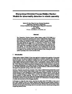
Figure 3: Figures (A), (B) and (C) report the smoothed correlation matrices between the monthly number of weapon offences across eight cities of the NSW state (Australia) at dates: i) January, 1995, ii) June, 2005, and iii) January, 2016, respectively. Figure (D) reports the correlation matrix implied by the limiting distribution. Results are reported relative to the Hierarchical Hidden Markov model with J = 4 and K = 3, estimated during the period January, 1995 – January, 2016.

25

Indeed, while at the beginning of the sample all series evolved following a similar path (see for instance at the begin of 1998), in the middle of the sample their movements became less correlated. To further investigate this aspect, we report in Figure 3 the smoothed correlation matrix at different time–periods. Specifically, Figure 3a reports the correlation matrix at the beginning of the sample in January 1995, while Figures 3b and 3c at the middle (June, 2005) and at the end (January, 2016) of the sample, respectively. We observe that the dependence structure across the series has changed during the observation time, as previously noted. The last Figure 3d reports the correlation matrix implied by the limiting distribution of the series. We see that, in the limit, all cities exhibit positive correlation in the rage 0.2 – 0.7. 6.2. Model’s goodness of fit To conclude our in–sample analysis, we investigate the model’s goodness of fit. Figure 4 reports a comparison between the limiting distribution of each city and the corresponding empirical one. We note that these distributions are heterogeneous among them, yet the estimated model is able to accommodate this feature. Univariate limiting distributions are computed starting from the joint limiting distribution - estimated by the HHMM with J = 4 and K = 3 components - as detailed in the following proposition. Proposition 5. Univariate distributions in the Hierarchical Hidden Markov Model The pmf of the univariate conditional random variable Yi,t |Y1:t−1 is given by: p(yi,t |Y1:t−1 ) =

J X j=1

πj,t|t−1

K X

ωj,k p(yi,t |St = j, Zt = k),

(28)

k=1

where p(yi,t |St = j, Zt = k) is the pmf of a Poisson distribution with intensity parameter λj,k,i for all i = 1, . . . , N . The unconditional distribution of the random variables Yi,t , for all i = 1, . . . , N , are computed replacing πj,t|t−1 in (28) with the stationary probabilities πj,∞ , for all j = 1, . . . , J. Proposition 5 states that univariate conditional and unconditional distributions in the Hierarchical Hidden Markov Model are a mixture of mixtures of univariate Poisson distributions. 26

0.030

0.04

0.05

0.025

0.04

0.020 0.015

0.03

0.010

0.02

0.005

0.01

0.000

0.03 0.02 0.01

0.00 20

40

60

80

0.00

100

0

(a) Sydney

10

20

30

40

0

(b) Newcastle

0.12

10

20

30

40

50

60

(c) Wollongong

0.10

0.10

0.08

0.08

0.08

0.06

0.06

0.06 0.04

0.04

0.04

0.02

0.02

0.02

0.00

0.00

0.00 0

5

10

15

20

25

30

35

0

(d) Tweed

5

10

15

20

25

0

(e) Coffs Harbour

10

20

30

40

(f) Albury

0.10

0.06

0.08 0.04

0.06 0.04

0.02

0.02 0.00

0.00 0

10

20

30

40

50

0

(g) Wagga Wagga

5

10

15

20

25

(h) Tamworth Regional

Figure 4: This figure reports a comparison between the empirical and limiting distribution of the number of monthly weapon offences in eight cities of the NSW State (Australia) over the sample January, 1995 – January, 2016. Results are reported relative to the Hierarchical Hidden Markov model with J = 4 and K = 3 components. The histograms indicate the empirical distribution, while the red lines the estimated ones.

27

B

Sydney

Newcastle

Wollongong

Tweed

Coffs Harbour

Albury

Wagga Wagga

Tamworth Regional

Critical Value

Panel (a) 195

0.16

0.07

0.23

0.10

0.17

0.16

0.11

0.12

0.35

200

0.16

0.06

0.23

0.10

0.17

0.16

0.12

0.13

2.73

205

0.17

0.06

0.23

0.10

0.17

0.16

0.12

0.13

5.89

210

0.18

0.06

0.23

0.10

0.17

0.16

0.13

0.13

9.39

215

0.18

0.06

0.23

0.10

0.17

0.16

0.13

0.14

13.09

220

0.18

0.06

0.23

0.11

0.17

0.16

0.13

0.14

16.93

Panel (b) 195

0.33

0.19

0.25

0.11

0.09

0.13

0.16

0.08

0.35

200

0.34

0.19

0.25

0.11

0.09

0.14

0.17

0.08

2.73

205

0.34

0.19

0.26

0.11

0.09

0.14

0.17

0.08

5.89

210

0.34

0.20

0.26

0.11

0.09

0.14

0.17

0.08

9.39

215

0.35

0.20

0.26

0.11

0.09

0.14

0.17

0.08

13.09

220

0.35

0.20

0.25

0.12

0.09

0.14

0.17

0.08

16.93

Table 4: χ2 test statistic values for the comparison between the empirical distribution of each series and its estimate according to the HHMM with J = 4 and K = 3 components. The null hypothesis is the equivalence between the P 2 empirical and estimated distributions. The statistic is computed as B b=1 (fb − 1/B) /(1/B), where B is the number

with F¯ (u) being the average conditional PIT computed as in Equation (3) of Czado of bins and fj = F¯ Bb − F¯ b−1 B et al. (2009). Panel (a) reports results for the conditional distributions p(yi,t |y1:t−1 ), while Panel (b) reports results for the unconditional distributions p(yi,t ) for i = 1, . . . , 8. Univariate distributions are computed starting from the joint distribution as detailed in Proposition 5. The statistic is approximately distributed as a χ2B−L , where L = 192 is the number of estimated parameters. The last column of the table reports the critical values at the 5% confidence level. Results are reported for different choices of B. Associated p–values are higher than 95% when B = 195 and higher than 99% for greater values of B.

In order to statistically assess the model’s fit, we compute the nonrandomized yet uniform Probability Integral Transform (PIT) for discrete variables defined in Czado et al. (2009) for each univariate time series. These are subsequently compared with the theoretical uniform distribution exploiting a standard χ2 test, where the null hypothesis is the equivalence between the empirical and

28

PB

− 1/B)2 /(1/B), where B is the

¯ number of bins in which the distribution is divided, and fj = F¯ Bb − F¯ b−1 B , with F (u) being the estimated distributions. The test statistic is computed as

b=1 (fb

average conditional PIT computed as in Equation (3) of Czado et al. (2009) for some u ∈ [0, 1]. Test statistics are reported in Table 4 for each univariate series. Panel (a) reports results for the conditional distributions p(yi,t |y1:t−1 ), while Panel (b) reports results for the unconditional distributions p(yi,t ), for i = 1, . . . , N . The statistic is approximately distributed as a χ2B−L , where L = 192 is the number of estimated parameters. The last column of the table reports the critical values at the 5% confidence level. In order to have positive degrees of freedom, we must have B > 192. Results are reported for B = {195, 200, 205, 210, 215, 220}. Associated p–values are higher than 95% when B = 195, and higher than 99% for greater values of B. 6.3. An index for prohibited and regulated weapon offences in NSW State An effective way of representing the overall criminal offences in NSW state is by the mean of an index. We build the prohibited and regulated weapon offences index as follows:

It = ξ 0 Yt ,

(29)

where ξ = (ξ1 , . . . , ξN ) is a vector of length N containing the weights associated to each city Yi,t ,

i = 1, . . . , N . For simplicity, here we set ξi = 1 for all i = 1, . . . , N such that our crime index,

It , is just the sum of the crimes committed in each city. We easily derive that:

Et−s [It ] = ξ 0 µt|t−s ,

(30)

V art−s [It ] = ξ 0 Et−s [Yt Yt0 ]ξ − ξ 0 µt|t−s µ0t|t−s ξ,

(31)

where Et−s [Yt Yt0 ] is reported in Section 3.2. As for Yt , predictive (s > 0), filtered (s = 0) and smoothed (s < 0) moments can be computed. Figure 5 reports the smoothed estimate of the index along with confidence interval bands.

29

200

150

100

50

95

97

99

01

03

05

07

09

11

13

15

Figure 5: Smoothed weapon offences index during the period January, 1995 – January, 2016. The index is computed as the sum of the number of monthly offences of eight cities in the NSW state (Australia). The cities are: Sydney, Newcastle, Wollongong, Tweed, Coffs Harbour, Albury, Wagga Wagga and, Tamworth Regional. Results are reported relative to the Hierarchical Hidden Markov model with J = 4 and K = 3. One standard deviation confidence bounds are reported.

We see that the overall level of weaponoffences has dramatically increased during the last twenty years. Indeed, shifting from about 60 to about 184, the index value has increased of approximately 300%. This piece of evidence indicates that a policy intervention to reduce the number of weapon offences should be considered. Planning an intervention for all cities can be difficult and time–consuming.

However, the

policymaker can exploit the dependence structure across the various cities and plan an intervention just in few of them. Given that our model predicts a limiting distribution of weapon offences exhibiting positive correlation among all the cities (see Figure 3d), other cities will also be indirectly affected by this intervention. 30

From now on, we focus on the predictive value of the index IT +h|T = ET [IT +h ] and the predictive value of the index given an intervention in city Yl,t , IT∗ +h|T = ET [IT +h |Yl,T +h ≤ kT +h ], where kT +h is a pre–specified upper bound for the number of offences in city l.4 The rationale behind the intervention is to define an upper bound for the future number of weapon offences in one city, and let the others benefit from this intervention based on the existing (predicted) mutual association. Although, entering into details of what the intervention might be goes beyond the scope of the paper, increasing the police budget or lower the weapons availability can be examples of possible interventions. Proposition 6. Expected value of the index conditional on an intervention Let IT∗ +h|T = E[IT +h |Y1:T = y1:T , Yl,T +h ≤ kT +h ], we have that: IT∗ +h|T

=

J X

∗ πj,T +h|T

j=1

K X k=1

ωj,k

N X

ξi λ∗j,k,i ,

(32)

i=1

where λ∗j,k,i = λj,k,i if i 6= l, and: λ∗j,k,i

Pkt+h =

b=1 bP (Yl,T +h = b|ST = j, ZT = k) , P (Yl,T +h ≤ kT +h |ST = j, ZT = k)

(33)

∗ otherwise, and πj,T +h|T = P (ST +h = j|Y1:T = y1:T , Yl,T +h ≤ kT +h ) is given by:

PJ

∗ πj,T +h|T

=

PK h q=1 αj,T [Γ ]q,j k=1 ωj,k P (Yl,T +h ≤ PJ PJ PK h n=1 p=1 αnt [Γ ]n,p k=1 ωpk P (Yl,T +h

kT +h |ST +h = j, ZT = k) ≤ kT +h |ST +h = p, ZT = k)

,

(34)

where P (Yl,T +h ≤ kT +h |ST = j, ZT = k) is the cumulative mass function of a Poisson distribution with parameter λj,k,i evaluated in kT +h . From Proposition 6 we note that the intervention kT +h influences both the expected value of the l–th series conditional con the realization of the two latent variables as well as the predictive probabilities of the Markov chain. 4

The generalization to more cities follows straightforwardly.

31

200 180 160 140 120 100 80 15

16

17

18

Figure 6: This figure reports the NSW state weapon offences monthly index prediction from February, 2016 to January, 2018. The start of the prediction is indicated by a black vertical line. The red dashed line indicates the index prediction without a policy intervention. The blue dashed line indicates the prediction conditional of an intervention in Newcastle of magnitude η = 0.1. The two blue dotted and dash–dot lines report predictions according to the two levels on intervention η = 0.3 and η = 0.5, respectively. An intervention is defined as a decrease of the number of weapon offences in Newcastle of at least η% with respect to the mean of weapon offences in 2 years from the end of the sample.

The choice of the city in which the intervention should take place can be based on political arguments. For instance, Sydney is the biggest city and, at the end of the sample, contributes to the 30% of the index’s value. However, making an intervention in Sydney, such as increasing the number of police agents, can be too expensive. We follow a statistical criterion and select the intervention city as the one being most correlated with other cities in the limiting distribution. This scheme indicates Newcastle which, on average, correlates 32% with other cities and, at the end of the sample, contributes by 10% to the index.

32

140 120 100 80 60 40 20 0

η = 0% η = 5% η = 10% η = 15% η = 20% η = 25% η = 30% η = 35% η = 40% η = 45% η = 50%

(a) Index Values

50 40 30 20 10 0

η = 0% η = 5% η = 10% η = 15% η = 20% η = 25% η = 30% η = 35% η = 40% η = 45% η = 50%

(b) Index Gains

Figure 7: Figure (A) reports the prediction of the NSW state (Australia) monthly weapon offences index at January, 2018 conditional on an intervention of size η in Newcastle. An intervention is defined as a decrease of the number of weapon offences in Newcastle at the end of the prediction of at least η% with respect to the mean of weapon offences at the end of the sample, with η = 0% indicating no intervention. Figure (B) reports the index gains. Index gains are defined as minus the percentage change in the prediction conditional on a particular intervention.

33

We select kT +h = (1 − η)µl,T |T for η ∈ (0, 1), and µl,T |T being the filtered mean of weapon offences in Newcastle at the end of the sample. That is, the target of the intervention is to reduce the number of weapon offences in Newcastle by at least a fraction η. We set h = 24 months and let kT +i for i = 1, . . . , h − 1 to linearly converge to kT +h such that the target is gradually reached. Figure 6 compares the index prediction without the intervention and its value conditional on the three types of intervention η = 0.1, 0.3, 0.5. We see that the impact of the intervention is high even when η is low, indicating that a small reduction in the number of weapon offences in Newcastle can have big impacts on the overall NSW State area. To gain further insights on the impact of the intervention, in Figures 7a and 7b we report the prediction of the index at January, 2018 and its percentage reduction for a grid of values for η, respectively. Interestingly, we find that an intervention in Newcastle, with a target decrease of at least 5% in two years, would induce a drop of the overall index value from 133.9 to 106.3 - a reduction of about 20.7%. Recall that Newcastle contributes only 10% in the index evaluation at the end of the sample. Increasing the level of the intervention, the index value continues to diminish. If the policymaker was able to reduce the number of weapon offences in Newcastle by a minimum of 50%, a similar decrease would be observed in other cities of the NSW state.

7. Conclusion This article showed that flexible dynamic modeling of multivariate nonnegative integer–valued time–series is possible with Hierarchical Hidden Markov models. Whereas the Markov latent variable captures time dependencies, the static latent variable models cross–dependencies, as well as additional features of the data within each Markov regime. The number of states and the number of components, if no prior knowledge is available, can be chosen based on well–known information criteria (like AIC or BIC). We have worked out the statistical properties of the model, and provided an EM algorithm for ML estimation. The latter, as results from the Monte Carlo experiment indicate, has showed good

34

performances in finite samples. In the empirical example, we have derived an index of criminal offenses for the NSW State (Australia), and showed that the correlation structure allowed by the model is able to predict how a policy intervention on one city affects the others. Specifically, we assumed a targeted intervention in the city being most correlated with the others, Newcastle, aimed at reducing the number of crimes of at least 5% in a two–year horizon. The model predicted, by the end of the intervention, a reduction of more than 20% in the overall crime index. Under the hierarchical modeling scenario presented in this paper, we have opted for the least restrictive structure possible: each Markov state is allowed to directly affect both the latent variable Zt and Y. Whereby enhancing model flexibility, this creates an overlap in the latent variable definitions, in that serial dependence affects also the definition of Zt . However, a constrained version of the model is also possible, in which the Markov states only affect Zt . Investigating what is the price, for enhanced model interpretation, the researcher has to pay in terms of loss of flexibility is an interesting topic for future research. Several other applications and extensions of the model we have proposed are possible. For instance, the performance of the model in forecasting applications can be investigated, whereas possible extensions of the current model might 1) accommodate for zero–inflated nonnegative integer– valued time–series, 2) allow for variables of mixed type, or 3) include time–constant and time–varying exogenous regressors.

Acknowledgments We would like to thank Jeroen K. Vermunt and Antonello Maruotti for insightfull comments on the paper and interesting suggestions for future works. We are also grateful to Rob Hyndman, Salvatore Ingrassia, Nicola Loperfido, Robert Jung, Antonio Punzo and Tommaso Proietti, for their comments.

35

Appendix A. Proofs Proof. Proposition 1 Recalling that P (St+h = j|St = i) corresponds to the i, j–th element of the matrix Γh denoted by [Γh ]i,j , we write:

P (St+h = j, Y1:t = y1:t ) P (Y1:t = y1:t ) PJ P (St = i, Y1:t = y1:t )P (St+h = j|St = i) = i=1 P (Y1:t = y1:t ) PJ h αi,t [Γ ]i,j = i=1 , PJ j=1 αj,t

P (St+h = j|Y1:t = y1:t ) =

(A.1)

in matrix form the vector of h–step ahead predicted probabilities becomes π t+h|t = α0t Γh /(α0t 1).

Proof. Proposition 2

P (Yt+h = yt+h |Y1:t = y1:t ) = =

P (Yt+h = yt+h , Y1:t = y1:t ) P (Y1:t = y1:t ) PJ PJ i=1 P (Y1:t = y1:t , St = j)P (St+h = i|St = j)P (Yt+h = yt+h |St = i) j=1 P (Y1:t = y1:t ) PJ

= =

j=1

PJ

h

i=1 αj,t [Γ

]j,i P (Yt+h = yt+h |St = i)

P (Y1:t = y1:t ) α0t Γh Pt+h 1 α0t 1

(A.2)

Proof. Proposition 3

First note that: 36

0

MYt (u) = E[eu Yt |Y1:t−1 = y1:t−1 ]

(A.3)

0

= E[E[eu Yt |St ]|Y1:t−1 = y1:t−1 ] =

J X

(A.4)

0

πj,t|t−1 E[eu Yt |St = j]

(A.5)

j=1 0

then by again applying the low of total expectation on E[eu Yt |St = j]:

0

0

E[eu Yt |St ] = E[E[eu Yt |St , Zt ]] =

K X

(A.6)

0

ωj,k E[eu Yt |St = j, Zt = k]

(A.7)

k=1

exploiting the conditional independence of the components of Yt :

0

E[eu Yt |St = j, Zt = k] =

N Y

E[eYi,t ui |St = j, Zt = k]

i=1 PN

=e since E[eYi,t ui |St = j, Zt = k] = eλj,k,i (e

ui −1)

i=1

λj,k,i (eui −1)

(A.8) (A.9)

is the moment generating function of a Poisson

distributed random variable. When substituting, we recover:

MYt (u) =

J X j=1

πj,t|t−1

K X k=1

which completes the proof.

Proof. Proposition 4 We first write:

37

PN

ωj,k e

i=1

λj,k,i (eui −1)

,

(A.10)

0 0 Cov(Yt , Yt−τ ) = E[Yt Yt−τ ] − E[Yt ]E[Yt−τ ],

(A.11)

we indicate by µ∞ the expected value of Yt which does not depend from t, hence E[Yt ] = E[Yt−τ ]. 0 The formula for E[Yt Yt−τ ] is evaluated by iteratively applying the low of total expectations and the

conditional independence of Yt |St from Yt−τ |St−τ as follows:

0 0 E[Yt Yt−τ ] = E[E[Yt Yt−τ |St , St−τ ]]

=

J X J X

(A.12)

0 E[Yt Yt−τ |St = j, St−τ = h]P (St = j, St−τ = h)

(A.13)

0 E[Yt Yt−τ |St = j, St−τ = h]P (St = j|St−τ = h)P (St−τ = h)

(A.14)

0 E[Yt Yt−τ |St = j, St−τ = h][Γτ ]h,j πh,∞

(A.15)

0 E[Yt |St = j]E[Yt−τ |St−τ = h][Γτ ]h,j πh,∞

(A.16)

j=1 h=1

=

J X J X j=1 h=1

=

J X J X j=1 h=1

=

J X J X j=1 h=1

=

J X K X J X K X

πh,∞ [Γτ ]h,j ωj,k ωh,b λj,k λ0h,b

(A.17)

j=1 k=1 h=1 b=1

Proof. Proposition 5 The proof is analogous for the conditional (Yi,t |Y1:t−1 ) and unconditional (Yi,t ) distributions for all i = 1, . . . , N . We simply condition on the two latent variables St and Zt and exploit the local independence between Yi,t and Yl,t for all l 6= i as follows:

p(yi,t |Y1:t−1 ) =

J X j=1

πj,t|t−1

K X k=1

then we note that: 38

ωj,k p(yi,t |St = j, Zt = k),

(A.18)

p(yi,t |St = j, Zt = k) =

p(yt |St = j, Zt = k) [−i] p(yt |Yi,t = yi,t , St = j, Zt

[−i]

,

(A.19)

= k)

[−i]

= (y1,t , . . . , yi−1,t , yi+1,t , . . . , yN,t )0 . Since p(yt |Yi,t = yi,t , St = j, Zt = k) = Q Q [−i] p(yt |St = j, Zt = k) = l6=i p(yl,t |St = j, Zt = k) and p(yt |St = j, Zt = k) = N m=1 p(ym,t |St = where yt

j, Zt = k), then p(yi,t |St = j, Zt = k) is simply the pmf of a univariate Poisson distribution with intensity λj,k,i .

Proof. Proposition 6 Let IT∗ +h|T = E[IT +h |Y1:T = y1:T , Yl,T +h ≤ kT +h ], we write:

IT∗ +h|T =

J X

∗ πj,T +h|t

j=1

=

J X j=1

J X

ωj,k E[IT +h |Y1:T = y1:T , Yl,T +h ≤ kT +h , ST +h = j, ZT +h = k]

(A.20)

h=1 ∗ πj,T +h|t

J X

ωj,k

h=1

N X

ξi E[Yi,t+h |Yl,T +h ≤ kT +h , ST +h = j, ZT +h = k]

(A.21)

i=1

∗ where πj,T +h|t = P (ST +h=j |Y1:T = y1:T , Yl,T +h ≤ kT +h ). From Remark 1, we have that, if i 6= l:

E[Yi,t+h |Yl,T +h ≤ kT +h , ST +h = j, ZT +h = k] = E[Yi,t+h |ST +h = j, ZT +h = k] = λj,k,i .

(A.22) (A.23)

In the case i = l, we have:

kT +h

E[Yl,T +h |Yl,T +h ≤ kT +h , ST +h = j, ZT +h = k] =

X

bP (Yl,T +h = b|Yl,T +h ≤ kT +h , ST +h = j, ZT +h = k)

b=1

(A.24) PkT +h

b=1 bP (Yl,T +h = b|ST +h = j, ZT +h = k) (A.25) P (Yl,T +h ≤ kT +h |ST +h = j, ZT +h = k)

= 39

In order to derive the predictive distribution of the Markov chain we write:

∗ πj,T +h|t = P (ST +h=j |Y1:T = y1:T , Yl,T +h ≤ kT +h )

=

P (ST +h=j , Y1:T = y1:T , Yl,T +h ≤ kT +h ) P (Y1:T = y1:T , Yl,T +h ≤ kT +h )

(A.26) (A.27) (A.28)

The denominator reads:

P (Y1:T = y1:T , Yl,T +h ≤ kT +h ) = P (Y1:T = y1:T , Yl,T +h ≤ kT +h |ST , ST +h )P (ST , ST +h )

(A.29)

= P (Y1:T = y1:T , Yl,T +h ≤ kT +h |ST , ST +h )P (ST +h |ST )P (ST ) (A.30) = P (Y1:T = y1:T |ST )P (Yl,T +h ≤ kT +h |ST +h )P (ST +h |ST )P (ST ) (A.31) = P (Y1:T = y1:T , ST )P (Yl,T +h ≤ kT +h |ST +h )P (ST +h |ST ) =

J X

J X αT (b) [Γh ]b,j P (Yl,T +h ≤ kT +h |ST +h )

=

(A.33)

j=1

b=1 J X

(A.32)

J K X X h αT (b) [Γ ]b,j ωj,k P (Yl,T +h ≤ kT +h |ST +h , ZT +h = k) j=1

b=1

k

(A.34) Following the same arguments, the numerator reads:

P (ST +h=j , Y1:T = y1:T , Yl,T +h ≤ kT +h ) = P (Yl,T +h ≤ kT +h |ST +h=j )

J X

αT (b)[Γh ]b,j

(A.35)

b=1

=

J X

αT (b)[Γh ]b,j

b=1

K X

ωj,k P (Yl,T +h ≤ kT +h |ST +h=j , ZT +h = k)

k

(A.36) 40

Substituting (A.29) and (A.35) in (A.26) we find: PJ

∗ πj,T +h|T

=

PK h q=1 αjt [Γ ]qj k=1 ωj,k P (Yl,t+h ≤ kt+h |St+h = j, Zt = k) PJ PJ PK h k=1 ωpk P (Yl,t+h ≤ kt+h |St+h = p, Zt = n=1 p=1 αnt [Γ ]np

which completes the proof.

41

k)

,

(A.37)

References Aitkin, M. (1996). A general maximum likelihood analysis of overdispersion in generalized linear models. Statistics and computing, 6(3):251–262. Al-Osh, M. and Alzaid, A. (1987). Firstorder integervalued autoregressive process. Journal of Time Series Analysis, 8(3):261–275. Bartolucci, F. and Farcomeni, A. (2009). A multivariate extension of the dynamic logit model for longitudinal data based on a latent markov heterogeneity structure. Journal of the American Statistical Association, 104:816–831. Bartolucci, F., Farcomeni, A., and Pennoni, F. (2012). Latent Markov models for longitudinal data. Chapman and Hall / CRC Press. Bartolucci, F., Montanari, G., and Pandolfi, S. (2015). Three–step estimation of latent markov models with covariates. Computational Statistics and Data Analysis, 83:287 – 301. Bartolucci, F., Pennoni, F., and Francis, B. (2007). A latent markov model for detecting patterns of criminal activity. Journal of the Royal Statistical Society: Series A (Statistics in Society), 170(1):115–132. Bu, R. and McCabe, B. (2008). Model selection, estimation and forecasting in inar (p) models: a likelihood-based markov chain approach. International journal of forecasting, 24(1):151–162. Bulla, J. and Berzel, A. (2008). Computational issues in parameter estimation for stationary hidden markov models. Computational Statistics, 23(1):1–18. Bulla, J., Chesneau, C., and Kachour, M. (2017). A bivariate first-order signed integer-valued autoregressive process. Communications in Statistics-Theory and Methods, 46(13):6590–6604. Collins, L. M. and Lanza, S. T. (2010). Latent class and latent transition analysis: With applications in the social, behavioral, and health sciences, volume 718. Wiley. 42

Czado, C., Gneiting, T., and Held, L. (2009). Predictive model assessment for count data. Biometrics, 65(4):1254–1261. Dempster, A. P., Laird, N. M., and Rubin, D. B. (1977). Maximum likelihood from incomplete data via the em algorithm. Journal of the royal statistical society. Series B (methodological), pages 1–38. Di Mari, R. and Bakk, Z. (2017). Mostly harmless direct effects: a comparison of different latent markov modeling approaches. Structural Equation Modeling: A Multidisciplinary Journal. Di Mari, R., Oberski, D. L., and Vermunt, J. K. (2016). Bias–adjusted three–step latent markov modeling with covariates. Structural Equation Modeling: A Multidisciplinary Journal, 23(5):649– 660. Doukhan, P., Fokianos, K., Støve, B., and Tjøstheim, D. (2017). Multivariate Count Autoregression. ArXiv e-prints. Fokianos, K., Rahbek, A., and Tjstheim, D. (2009). Poisson autoregression. Journal of the American Statistical Association, 104(488):1430–1439. Fr¨ uhwirth-Schnatter, S. (2006). Finite mixture and Markov switching models. Springer Science & Business Media. Geweke, J. and Amisano, G. (2011). Hierarchical markov normal mixture models with applications to financial asset returns. Journal of Applied Econometrics, 26(1):1–29. Hamilton, J. D. (1994). Time series analysis, volume 2. Princeton university press Princeton. Jones, C., Kypri, K., Moffatt, S., Borzycki, C., and Price, B. (2009). The impact of restricted alcohol availability on alcohol–related violence in newcastle, nsw. NSW Bureau of Crime Statistics and Research. Jørgensen, B., Lundbye-Christensen, S., Song, P.-K., and Sun, L. (1999). A state space model for multivariate longitudinal count data. Biometrika, 86(1):169–181. 43

Jung, R. C., Liesenfeld, R., and Richard, J.-F. (2011). Dynamic factor models for multivariate count data: An application to stock-market trading activity. Journal of Business and Economic Statistics, 29(1):73–85. Karlis, D. (2015). Models for multivariate count time series, pages 407–424. Chapman & Hall: Boca Raton, FL. Karlis, D. and Pedeli, X. (2013). Flexible bivariate inar (1) processes using copulas. Communications in Statistics-Theory and Methods, 42(4):723–740. Kocherlakota, S. and Kocherlakota, K. (1992). In editor, T., editor, Bivariate Discrete Distributions, Statistics: Textbooks and Monographs, volume 132. Markel Dekker, New York. Maruotti, A. and Ryd´en, T. (2008). A semiparametric approach to hidden markov models under longitudinal observations. Statistics and Computing, 19(4):381. McKenzie, E. (1988). Some arma models for dependent sequences of poisson counts. Advances in Applied Probability, 20(4):822–835. McLachlan, G. and Peel, D. (2000). Finite mixture models. John Wiley & Sons. Nelsen, R. B. (2006). An Introduction to Copulas, 2nd edn. SpringerVerlag, New York. Olteanu, M. and Rynkiewicz, J. (2012). Asymptotic properties of autoregressive regime-switching models. ESAIM: PS, 16:25–47. Pedeli, X. and Karlis, D. (2011). A bivariate INAR (1) process with application. Statistical modelling, 11(4):325–349. Pedeli, X. and Karlis, D. (2013a). On composite likelihood estimation of a multivariate INAR (1) model. Journal of Time Series Analysis, 34(2):206–220. Pedeli, X. and Karlis, D. (2013b). Some properties of multivariate INAR (1) processes. Computational Statistics and Data Analysis, 67:213–225. 44

Redner, R. A. and Walker, H. F. (1984). Mixture densities, maximum likelihood and the em algorithm. SIAM review, 26(2):195–239. Rydberg, T. H. and Shephard, N. (1999). A modelling framework for the prices and times of trades made on the new york stock exchange. Scotto, M. G., Weiss, C., and Gouveia, S. (2015). Thinning–based models in the analysis of integervalued time series: a review. Statistical Modelling, 15(6):590–618. Vermunt, J. and Magidson, J. (2004). Factor analysis with categorical indicators: A comparison between traditional and latent class approaches, pages 41–63. Mahwah, NJ: Erlbaum. Vermunt, J. K. (2010). Latent class modeling with covariates: Two improved three-step approaches. Political Analysis, 18:450–469. Vermunt, J. K., Langeheine, R., and B ockenholt, U. (1999). Discrete-time discrete-state latent markov models with time-constant and time-varying covariates.

Journal of Educational and

Behavioral Statistics, 24:179–207. Weatherburn, D., Jones, C., Freeman, K., and Makkai, T. (2003). Supply control and harm reduction: lessons from the australian heroin drought. Addiction, 98(1):83–91.

45