High Performance Computing With .NET

High Performance Computing With .NET Enabling .NET as efficient platform for numerical computations

Haymo Kutschbach TU-Berlin, ILNumerics

For the development of numerical algorithms scientists can choose from a wide spectrum of popular tools. Due to their specialization, those tools are well prepared to support the design and verification of such algorithms for a nearly infinite large range of academic and industrial domains. However, the production flow does not end with the working method. The intrinsic knowledge about mathematical routines must get incorporated into real world programs, shipped to customers, run on computers with a whole range of different hardware configurations, maintained as part of a larger application — possibly by a whole development team and verified within testing frameworks — short: all requirements of a professional software development lifecycle apply. This is where most specialized frameworks lack reliable support. Several attempts have been made to close that gap, mostly on the side of mathematical tools — without succeeding completely. This work describes a different approach. The most popular general purpose language (C#) for one of the most popular software development frameworks for business applications nowadays (.NET) is extended with a library for convenient description and efficient execution of numerical algorithms. The structure of the work itself reflects the most common steps for professional software development: analysis, design, implementation and verification. One goal of the work is to investigate the options the .NET platform offers for high performance numerical computing as well as the potential enhancements provided by extensions to the framework. This work will focus the .NET framework, not accounting the potential other managed frameworks bring — namely Java and Python. However, in the analysis part comparisons are made between .NET and Java regarding the most important requirements identified for numerical computations. The choice of .NET over Java will be motivated as well.

R

This work has been supported by idalab GmbH and TU-Berlin by providing Intel compiler technology and access to MATLAB instances for the performance comparisons contained within. R

Contents 1. Analysis 1.1. Programming Languages — Distinction by Purpose . 1.2. DSL Utilization . . . . . . . . . . . . . . . . . . . . . 1.2.1. Deployment Strategies for DSL Algorithms . 1.3. GPL Utilization . . . . . . . . . . . . . . . . . . . . . 1.4. Current and historic Approaches . . . . . . . . . . . 1.4.1. Javanumerics . . . . . . . . . . . . . . . . . . 1.4.2. Other Java Attempts . . . . . . . . . . . . . . 1.4.3. .NET Projects . . . . . . . . . . . . . . . . .

. . . . . . . .

. . . . . . . .

. . . . . . . .

. . . . . . . .

. . . . . . . .

. . . . . . . .

. . . . . . . .

. . . . . . . .

. . . . . . . .

. . . . . . . .

. . . . . . . .

5 . 5 . 5 . 5 . 7 . 9 . 9 . 9 . 10

2. Design Goals 2.1. Obligatory Requirements . . . . . . . . . . . . . . . 2.2. Syntax requirements . . . . . . . . . . . . . . . . . . 2.3. Supplementary Requirements . . . . . . . . . . . . . 2.4. Requirements for professional Software Development 2.5. Performance Design Goals . . . . . . . . . . . . . . . 2.5.1. Optimizations: Bound Check Removals . . . 2.5.2. Interfaces to native code . . . . . . . . . . . . 2.5.3. Parallel execution models . . . . . . . . . . . 2.5.4. Performance gains by design . . . . . . . . . 2.6. CLR Memory Management . . . . . . . . . . . . . . 2.6.1. Managed Heap and Generational GC . . . . . 2.6.2. Small Object Heap . . . . . . . . . . . . . . . 2.6.3. Large Object Heap . . . . . . . . . . . . . . . 2.6.4. Heap Fragmentation . . . . . . . . . . . . . . 2.6.5. Memory Management Conclusions . . . . . .

. . . . . . . . . . . . . . .

. . . . . . . . . . . . . . .

. . . . . . . . . . . . . . .

. . . . . . . . . . . . . . .

. . . . . . . . . . . . . . .

. . . . . . . . . . . . . . .

. . . . . . . . . . . . . . .

. . . . . . . . . . . . . . .

. . . . . . . . . . . . . . .

. . . . . . . . . . . . . . .

. . . . . . . . . . . . . . .

. . . . . . . . . . . . . . .

11 11 11 12 13 13 16 17 20 21 22 23 23 24 25 27

. . . . . . . .

29 29 29 29 30 32 32 34 34

3. Implementation 3.1. Overall Architecture . . . . . . . . . . . 3.2. Storage . . . . . . . . . . . . . . . . . . 3.2.1. Element Storage . . . . . . . . . 3.2.2. Wrapper Class Design . . . . . . 3.2.3. Subarray access, Expressions . . 3.2.4. Array Interaction and Mutability 3.3. Miscellaneous Features . . . . . . . . . . 3.3.1. Parallelization . . . . . . . . . .

. . . . . . . . . . . . . . . . . . . . Rules . . . . . . . .

. . . . . . . .

. . . . . . . .

. . . . . . . .

. . . . . . . .

. . . . . . . .

. . . . . . . .

. . . . . . . .

. . . . . . . .

. . . . . . . .

. . . . . . . .

. . . . . . . .

. . . . . . . .

. . . . . . . .

. . . . . . . .

4. Memory Management 37 4.1. Memory Management Overview . . . . . . . . . . . . . . . . . . . . . . . . 37

3

4.2. Memory Pool . . . . . . . . . . . . . . . . . . . . . . . . . . . . . . . . . . 37 4.3. Usage Rules . . . . . . . . . . . . . . . . . . . . . . . . . . . . . . . . . . . 39 4.3.1. Usage Rule I — Array Type Declarations . . . . . . . . . . . . . . 39 4.3.2. Usage Rule II — Artificial Scoping . . . . . . . . . . . . . . . . . . 40 4.3.3. Usage Rule III — Function Parameter Assignments . . . . . . . . 41 4.3.4. Usage Rule Example . . . . . . . . . . . . . . . . . . . . . . . . . . 41 4.4. Scoping and Deterministic Disposal . . . . . . . . . . . . . . . . . . . . . . 42 4.4.1. Input Parameter Handling . . . . . . . . . . . . . . . . . . . . . . . 43 4.4.2. Assignment Handling . . . . . . . . . . . . . . . . . . . . . . . . . 43 4.4.3. Return Value Handling . . . . . . . . . . . . . . . . . . . . . . . . 44 4.4.4. Handling Object Member Calls . . . . . . . . . . . . . . . . . . . . 44 4.4.5. Holes in the Scheme . . . . . . . . . . . . . . . . . . . . . . . . . . 44 4.5. Value Type Semantics . . . . . . . . . . . . . . . . . . . . . . . . . . . . . 45 4.6. Additional Output Parameters . . . . . . . . . . . . . . . . . . . . . . . . 45

5. Conclusion

47

A. Appendix

49

A.1. Memory Pool Activity Diagram . . . . . . . . . . . . . . . . . . . . . . . . 49 A.2. Performance Comparisons . . . . . . . . . . . . . . . . . . . . . . . . . . . 50 A.2.1. Comparison Overview . . . . . . . . . . . . . . . . . . . . . . . . . 50 A.2.2. ILNumerics Code . . . . . . . . . . . . . . . . . . . . . . . . . . . . 51 A.2.3. MATLAB Code . . . . . . . . . . . . . . . . . . . . . . . . . . . . . 52 A.2.4. FORTRAN Code . . . . . . . . . . . . . . . . . . . . . . . . . . . . 53 A.2.5. numpy Code . . . . . . . . . . . . . . . . . . . . . . . . . . . . . . 54 A.2.6. Test Setup . . . . . . . . . . . . . . . . . . . . . . . . . . . . . . . 54 A.2.7. Performance Results . . . . . . . . . . . . . . . . . . . . . . . . . . 56 A.3. Fragmentation Prevention by Pooling

. . . . . . . . . . . . . . . . . . . . 56

1. Analysis In this chapter we will evolve a motivation for a numerical library. The gap caused by different requirements for the scientific and for the industrial world will be outlined.

1.1. Programming Languages — Distinction by Purpose General purpose languages (GPL) basically means: ”The developer can do everything”. Such languages show little to no adaptation to any specific problem domain. They are designed and best suited to create deployable applications for any technically addressable purpose which actually run on a target computer with standard equipment. Some prominent examples are C/C++, Java, C#, Delphi and FORTRAN. Domain specific languages (DSL) are designed to address specific problems for a more narrow area of interest. Some DSL are defined as a subset of a GPL. They commonly use the same tools and compile to the same format as the corresponding GPL. These languages somehow blur the line between DSL and programming libraries for GPL1 . A popular example here is SciPy 2 . Other DSL are utilized within special application frameworks only. They often require not only individual development tools but also aim towards specialized runtime support in order to deploy and run inside an application on any computer. The most prominent examples here at the same time are known as some of the most widely spread environments for mathematical computations and algorithm development: MATLAB and Mathematica3 . R

1.2. DSL Utilization Scientists and mathematicians often prefer to profit from the advantages introduced by specialized mathematical DSL. Interactive environments support the development process with visualization and debugging capabilities. Short handed syntax helps the formulation of complex formulas in an efficient way. Often a large set of predefined mathematical functions enables one to reuse inherent knowledge in a reliable way. Mathematical DSL often are not strongly typed and focus on the formulation of algorithms in a functional or imperative form.

1.2.1. Deployment Strategies for DSL Algorithms From the software developer point of view it is crucial to implement an algorithm with respect to stability, maintainability and extensibility into a final product. It is important 1

A Formal Approach to Domain-Oriented Software Design Environments (PDF) SciPy relys on numpy which extends the python runtime. See: http://numpy.scipy.org 3 http://www.martinfowler.com/bliki/DomainSpecificLanguage.html 2

High Performance Computing With .NET - Kutschbach, 2012

5

1. Analysis for her to find the right balance of implementation and maintainability efforts and the overall costs of the full application lifecycle. The common choice will therefore be a GPL. Thus, in practice the need arises to incorporate an existing DSL algorithm into a deployable application. Major DSL frameworks provide the following options: 1. The algorithm is compiled from the DSL into any sort of module which is compatible to the GPL and therefore callable at runtime. An API is defined and used in order to connect to the module and utilize in parts the functionality provided by the DSL at runtime. Therefore, supporting parts of the DSL (e.g. optimization libraries and higher level functionality) need to be deployed within the final application. Changes to the algorithm commonly require the availability of the original DSL framework in order to recompile and deploy the whole module. Next to the dependence on the DSL framework, that approach brings further disadvantages: it increases deployment size, inherits platform restrictions from the algorithm module and possibly decreases runtime performance due to frequent transition between different execution models and increased memory dislocation. Furthermore, most mathematical DSLs do not confirm to the requirements for runtime safety, with the result of the final application inheriting the nuisances of the less stable runtime behaviour. One famous example of a DSL framework providing this deployment model is Mathworks’ MATLAB Compiler4 . The compiler can be used to create C code out of MATLAB script files — the DSL code of the MATLAB algebraic application. Among with several other libraries those C files can then get further incorporated into own applications. R

R

R

2. Another model of deployment for DSL algorithms is given by the example of Mathematica MathLink . The framework requires a specific standalone application (”Mathematica Kernel”) to exist on each target computer where the DSL programs (so called ”Notebooks”) are to be executed. Interaction between and control of that kernel is achieved via interprocess communication. R

3. A less intrusive way is given by R — a famous statistical computing environment5 . It publishes a number of C header file definitions and C style libraries which can be used to link against the R computational routines in the same way as known from standard application building with C. However, the API to the R framework resides on a much lower level than in the deployment models described above. Hence the user needs to keep track of proper contract fulfilment — including memory management of all created R objects. 4. In absence of other possibilities and as a last resort the algorithm can always manually be transformed into a GPL. This, at the same time, is the most flexible and probably also the most expensive way of incorporating a DSL algorithm. The costs can be limited by initially choosing a DSL, which due to its nature provides a fast and easy transition from the scientific representation to the syntax of the chosen GPL. The more both languages and the underlying architecture vary, the more effort needs to be spent for the complete transition process and the more error prone the translation will be. 4 5

6

http://www.mathworks.com/products/compiler http://www.r-project.org/about.html


1.3. GPL Utilization Most deployment models invest some effort to provide a similar DSL syntax even within the interfaces to GPLs. However, due to the very nature of DSL — being specialized and different from GPL in all mentioned cases — a break in the syntax consistency seems impossible to prevent. Even by specifying necessary data definitions and algorithm details for the computational model directly in the corresponding DSL by character strings (as accepted by Mathematica e.g.), external interactivity (data in-/output) of the models is not feasible except via the native ways provided by the GPL used. Therefore, by fulfilling the API between both worlds, the developer cannot circumvent the handling of both languages — each with its own quirks.

1.3. GPL Utilization All the problems described above can be prevented if the scientist relies on a GPL for algorithm development right from the start. One can choose from several options here. The most mature choice is FORTRAN. Developed around 1955 with the focus on numerical algorithm development, FORTRAN is said to be the first wide spread programming language at all, which was able to create programs for a large number of platforms. Over the years the language received several enhancements. Since simplified in- and output support in FORTRAN 77 (released 1978) and due to its wide compiler support for almost every platform existing, it often gets categorized as GPL rather than DSL. The most current version is FORTRAN 2008. Due to its low-level code optimizing features it still is the first choice among other numerical programming languages regarding execution speed and therefore is still often used in the area of high performance computing. FORTRAN was developed with the best possible execution speed performance in mind. The language provides special keywords which are used as hints for the compiler in order to help reduce instructions and optimize the program flow with intrinsic knowledge of the underlying algorithm. Due to its low-level descriptive capabilities, FORTRAN requires more technical experience from the developer than common high level DSL. Several other languages promise a good balance between the diverse goals in the supply of mathematical algorithms. Apart from FORTRAN, C/C++ is the other mature and even more popular language. Both compile to native platform specific code. The other category of modern GPL is comprised out of those languages which are destined to be compiled for virtual runtime environments. Languages for virtual runtime environments do not compile to machine code in the first place. The compilation step results in an intermediate language byte code which is specific to the environment but not to the target platform and mostly consists out of a reduced instruction set compared to the instruction sets for common CPUs. The runtime environment completes the translation of the instructions directly on the target machine — right before execution — just in time (JIT). Since for most such environments multiple implementations exist for several platforms, this concept can be seen as big step towards platform independence. Because the final compilation is done on the target machine, the JIT compiler could possibly utilize more specific optimizations than would be possible for a regular machine code compiler. Still, the execution speed of programs running in a virtual environment in general tends to be a little less optimized than possible and hence runs slower than in native programs. Most environments do implement a garbage collector which aims to save the developer from the need for individual memory management. The virtual


7

1. Analysis

Figure 1.1.: The number of job advertisements since 2005. The lines show the relation of the number of corresponding ads, filtered by individual keywords. (Source: indeed.com)

machine keeps track of objects which are no longer used and frees them automatically. Famous representatives are Java RT or Java Virtual Machine (JVM) with its corresponding languages, .NET (C#, Visual Basic, J#, C++/CLI, F# and IronPython), Python, Perl/PHP, Javascript and Smalltalk. The abstraction of program code from the physical hardware layer by the virtual machine is also reflected by the languages designed to run on such environments. Automatic memory management is only one example where the developer is strongly supported in writing more stable applications. The advantages are obvious: not only are those languages easy to learn, but writing a program is often faster and results in better maintainable code. Several approaches exist that utilize such languages for numerical applications. However, mostly due to the proposed slower execution speed, the acceptance within the scientific community is still relatively low6 . This work will develop another attempt to close the gap between the requirements for scientists and for software developers. By choosing a GPL for virtual environments which introduces the fewest missing features in favor of a numerical DSL and trying to implement enhancements, extensions and workarounds for all perturbing issues, we endeavour to get closest to the goal of making the virtual environment GPL a favourable language for the development and direct formulation of numerical algorithms. 6

8

An example for a popular language is found in numpy and related packages like scipy. While gaining more and more acceptance for prototyping algorithms, those ’script languages’ are not considered as stable alternatives for enterprise application development here. The reasons are found in their poor typesafety and deficient support in the management of larger projects — to name several.


1.4. Current and historic Approaches

1.4. Current and historic Approaches The thoughts presented in Chapter 1.3 are by no means new. The Java platform has been in the focus for enhancements towards numerical computing in the past much more often than the .NET platform. The most recognizable efforts are summarized here.

1.4.1. Javanumerics In 1998, the Java Grand Forum7 , a consortium of several industry partners (namely NIST, Mathworks, IBM, Visual Numerics, NAG, Intel and several universities worldwide) declared the goal of enhancing the Java platform to become the first choice for numerical computations8 . Several proposals have been created in meetings and conferences and the following design goals were identified: • Complex arithmetic, lightweight numbers, full range of supporting arithmetic functions • Fixed size, multidimensional, performant array classes9 • Improved syntax (operator overloading, subarray options) • Linear algebra, comparable to the Lapack10 package • Higher mathematical functions, working on the array classes • Strict floating point arithmetics11 The progress of the project stalled in 2003, possibly due to conflicting views among the forum members regarding the floating point issues and the low willingness of Sun (the formerly maintainer of Java) to incorporate any (even not potentially breaking) changes into the JVM1213 .

1.4.2. Other Java Attempts Next to the javanumerics project, several other projects were and still are aiming towards the same goals on the Java platform. Some of the apparently more visible attempts are: The Ninja Project14 — an effort by IBM research, Apache Commons Math15 , the Universal Java Matrix Package16 and jblas17 . The collection is not complete. While 7

See: http://javagrande.org See: http://math.nist.gov/javanumerics 9 See: http://www.jcp.org/en/jsr/detail?id=83 10 See: http://netlib.org/lapack 11 This demand handled the utilization of processor specific floating point instructions from within the Java language / the JRT. It also suggested potential implementation details to work around the nuisances of conflicting results among concurrent instruction sets: http://www.jcp.org/en/jsr/detail?id=84 12 See: http://cio.nist.gov/esd/emaildir/lists/jama/msg01332.html 13 See: http://osdir.com/ml/java.openjdk.compiler.devel/2006-12/msg00043.html 14 See: http://www.research.ibm.com/ninja/#ics00 15 See: http://commons.apache.org/math/ 16 See: http://sourceforge.net/projects/ujmp/ 17 See: http://jblas.org/ 8


9

1. Analysis the Ninja project focuses on execution speed improvements, the Apache project aims at providing higher level functionality. Further design goals besides those extracted from javanumerics could not be identified. The experiences with the javanumerics as well as the Ninja projects make it clear that in order to enable Java for serious numerical computing, substantial changes to the Java RT and the Java language would be required. Since even the open character of Java did not help to realize those efforts, chances are low they will be realized anytime soon. Around the same time the javanumerics project died, Microsoft released the .NET framework and the C# language started on the road to success in becoming one of the most recognizable languages for professional application development — next to Java.

1.4.3. .NET Projects The younger age of .NET is reflected by a smaller number of currently available numerical libraries for that platform. Popular implementations are provided by Rogue Wave18 , NAG19 , Centerspace20 , Math.NET Numerics21 and the project this work is based on: ILNumerics22 . Most projects are either open source or smaller parts of a vendor, creating compiler infrastructures and comprehensive sets of FORTRAN libraries. All but ILNumerics deviate considerably from the requirements elaborated in Section 2. C# is the youngest of all major virtual runtime environments GPL which received considerable acceptance within the community for middleware and multitier application developers. Released in 2001, it has caught up with C++ as far as job offering concerns23 in 2010. Targeting the .NET platform, C# is by far the most popular language. All projects listed here enable the utilization of C# as mathematical language with more or less comfortable features. Another popular .NET language for scientific computations is F# which due to its functional syntax style deviates from the attempts of this work in many aspects and hence is not further taken into account here. The vast majority of all numerical libraries in managed environments currently existing serve as a more ore less thin wrapper to underlying native libraries. This is true for both .NET and Java. We will not consider this approach here either since the computations would not really be carried out in the virtual language environment.

18

See: http://www.roguewave.com/ See: http://www.nag.co.uk/netdevelopers.asp 20 See: http://www.centerspace.net 21 See: http://mathnetnumerics.codeplex.com/ 22 See: http://ilnumerics.net 23 See: http://www.indeed.com/jobtrends — worldwide meta listing and comparison of jobs according to specific search phrases 19

10


2. Design Goals In this section more specific requirements for a framework for numerical application development are investigated. We will find they mostly match those identified by the javanumerics project. However, newer evolution steps in the computer architecture make some of them deviate towards different solutions, especially regarding execution speed, which is discussed in Section 2.5. While collecting specification bits we will keep the selection of a favourable language in mind. However, only the two most significant languages are considered from here on: Java and C#.

2.1. Obligatory Requirements • Correct, deterministic • Operator precedence, IEEE 754 conform floating point arithmetic • Capability of handling arrays These points are fulfilled by all prominent languages nowadays.

2.2. Syntax requirements From the mathematicians’ point of view, the language syntax is crucial. The following requirements are somehow arbitrarily chosen by the authors own experience and are oriented on the widely accepted MATLAB syntax. If we define the goal to get as close as possible to these syntax features, we can expect a steep learning curve for those scientists already familiar with (e.g.) MATLAB . The language should enable one to formulate the algorithms by use of tensor objects. Those objects should be flexible in creation and manipulation with the most possible compact notation. Arrays should be used to handle all orders of dimensionality: empty arrays, scalars, vectors, matrices and n-dimensional arrays. Two examples: R

R

A = rand ( 5 , 4 , 3 ) ∗ s q r t ( − 2 . 0 ) ; // t h r e e d i m e n s i o n a l a r r a y B ( : , 1 : 2 : end ) = A( 1 : end , : , end −1) + C ’ ; Array objects are provided by both, Java and C# and are capable of serving as mathematical variables of any size and dimensionality. Classes can be used on both platforms to encapsulate extended functionality for those objects. C# provides indexer which utilize brackets and can be used for subarray creation and subarray assignments on array objects. On the Java side there is no equivalent.


11

2. Design Goals Both languages support basic mathematical operators — for primitive types. C# allows the developer to overload such operators for classes as well1 . On the Java side there is no equivalent. Complex numbers are provided in .NET framework version 4.0. Unfortunately the implementation lacks of completeness2 . For Java, third party libraries exist3 . However, both frameworks bring the option to implement a custom solution and integrate those complex number classes seamlessly — with the exception of the lack of overloadable operators and lightweight classes (called ’structs’ in .NET) in the case of Java. Mathematical DSL commonly pass parameters for functions by value4 . This prevents code in one scope from accidentally changing arrays within the calling scope. Due to the nature of virtual environment languages in conjunction with the garbage collecting memory management as well as for efficiency reasons, parameters of complex types (i.e. instances of classes) are always passed as reference variables to function parameters. However, a special class design can be used to change that behaviour to one which appears to pass parameters by value. In order to make this work a lot of type conversions are necessary. Thus, another language feature of C# proves to be useful here: implicit conversion operators. For Java there is no equivalent. Similar to indexers, C# properties come in handy for transposing expressions and for shallow copies of an array. MATLAB provides the ’ operator: R

A’ % r e t u r n t r a n s p o s e o f A A.T // e q u i v a l e n t with C# p r o p e r t y i n ILNumerics Even if less intuitive, in Java a function could be used, to achieve the same result.

2.3. Supplementary Requirements Next to the syntax for algorithm formulation, some further important features are obligatory and common for scientist. The implementation should be enhanced by a collection of standard base algorithms for sorting, fast fourier transforms and linear algebra functionality. The design should enable the creation and extension of custom algorithms which must be easily reusable. Visualization capabilities should enable the creation and (re)use of interactive graphs in two and three dimensions. For the sake of simplicity and stability, the visualization solution should utilize standard GUI capabilities of the GPL and the corresponding runtime environment. Both platforms support OpenGL, Java again brings more options for 3rd party higher level 3D programming APIs. The development of algorithms should be enhanced by debugger support, adjusted for the specific requirements of numerical objects. The most mature and prominent integrated development environments for .NET and Java (Visual Studio and Eclipse) 1

with the only exception of the assignment operator. A limitation which will become important at a later point. 2 The .NET 4.0 System.Numerics.Complex data type supports only double precision numbers and lacks on support for several higher level functions. 3 http://commons.apache.org/math/ 4 The popular numpy package is one out of several exceptions. The reasons are found within the restrictions of the underlying GPL, here: python.

12


2.4. Requirements for professional Software Development are both highly configurable and provide several plug-in mechanisms for extensions of any purpose. Interfaces to modules created by use of other common GPL should exist and be utilizable in an efficient manner. Existing code therefore is able to get incorporated without necessary rewriting. Those parts of an algorithm which are most performance critical, can easily be enhanced by interfacing native, platform dependent optimized libraries, created by FORTRAN or C. The .NET platform offers the option to deviate from the strict safe programming guidelines, which enables one to even inject arbitrary machine instructions into the executing instruction flow with very little to no overhead5 .

2.4. Requirements for professional Software Development A list of minimal requirements to professional software targeting industrial applications might look as follows: • Easy and reliable deployment • Minimal number of additional dependencies • Large number of supported platforms • IO/Misc. framework – Compatible range of additional GP-framework functionality, file interaction, network connectivity, possibilities for the integration into multitier applications • Runtime error prevention, inherent stability of the language – Type safety, mechanisms of memory management • ’Good’ balance between: – Implementation cost – Execution speed – Maintainability – Extensibility Since the GPL state for both, C#/.NET (mono for other platforms than Windows) and Java is widely accepted, those requirements are fulfilled by definition.

2.5. Performance Design Goals The implementation should be competitive with and even bring higher performance than other common DSL. 5

The CLR allows the calling of unmanaged code by utilization of ”delegates” — the .NET function type. See: http://msdn.microsoft.com/en-us/library/system.runtime–.interopservices–.marshal–.getdelegateforfunctionpointer–.aspx or the Marshal–.GetDelegateForFunctionPointer() Method in the online documentation at http://msdn.microsoft.com


13

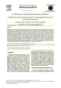
2. Design Goals In general, having two software systems within the same hardware system the one is said to be more performant, which is able to utilize available computing resources more efficiently. A rough measure for the performance of two different algorithms is execution time. The algorithm which finishes faster with the same (correct) result is considered to bring better performance. Other possible views on performance include the consumption of energy and — highly related hereto — the production of waste heat. The final speed of execution depends on a large number of influencing factors, including (but not limited to): • The number of instructions in the instruction stream to any processing unit of the processor(s). • The ability of the development tools involved to produce a final instruction stream which the processing resources are able to execute in a highly optimized way. • The success of those tools to anticipate and utilize available resources to the upmost extend. • The management and efficient utilization of supplementary system resources like I/O processing and data and instruction memory bandwith. In order to utilize available hardware resources efficiently the following principles are of importance: • Parallelization — most important targets of parallelization are the instruction stream (i.e. Instruction-Level Parallelism, Instruction Pipelining and Superscalar architectures, SIMD instructions like the SSE extensions on the x86 platform) and the higher level — or ”Thread Level Parallelism” by the utilization of multiple processing cores. At the same time, recent GPU processing offers even higher parallelization perspectives on a SIMD base. • Principle of locality. In Figure 2.1 the average growth in performance of processors and memory is shown for the computer architectures over the last 30 years. While processing units roughly doubled their performance every year until 2000, the speed of memory accesses increased by 1.07 per year only. This makes the memory access the major bottleneck and target for a large number of optimization attempts in both, hardware and software. One of the more important ones on the hardware side is the utilization of multilevel caches nearby processing units. They allow recently used data to be delivered to the processing registers much faster. Data which needs to be requested from main memory (or even from the pagefile on the harddisk) introduces a severe performance drop by stalling the execution unit, causing context switches and possibly increased contention in the case of multiple threads involved. ’Prefetching’ tries to extend the principle of locality to data that is more likely to be needed in the future. This principle is just as valid for data as for instructions. It must be taken into account by processor designers trying to optimize the memory throughput inside the processor as well as software architects (especially OS architects). In order to achieve peak performance for numerical algorithms, the programmer (or the supporting framework/ DSL) must consider this principle as well and support the underlying hard- and software in

14


2.5. Performance Design Goals optimizing for it. Figure 2.1 lists the typical cost of hits and misses for a first level cache and for virtual memory.

Figure 2.1.: Single processor performance trends against the trends in memory latency plotted over the time. Numbers were taken from: Hennesy, Patterson; Computer Architecture A Quantitative Approach, 5th Edition, Morgan Kaufman, 2011, page 73 R

Since in 2005, Intel at last turned away from single processor improvements towards multi core designs6 , the potential for future performance improvements has moved towards the principle of thread level parallelism. This also means that the programmer must take care of the utilization of this principle more than ever since the necessary parallelization of the algorithms must be done on a level too high for the processor to fullfill this task automatically. Another implication relates to one of the demands back from the javanumerics project. It was claimed that the utilization of (processor architecture specific) floating point extensions would be crucial for the improvement of Javas execution speed. The insights into the recent turns in processor architecture suggest a wider perspective: It appears not to be any single processor feature which is crucial here, but the utilization of multiple processing units — at most the conjunction of both options. However, the profit of utilization of floating point extensions will likely be overcome by the increase rate of multi core/ GPU architectures in the time span of a few design generations. We identify the following areas of optimization potential: • Reduction of instructions, 6

See Figure 2.1 — since 2005 no relevant increase in performance on a single processor core could be achieved.


15

2. Design Goals First-level cache

Virtual memory

Block size / page size

16B -128B

4KB - 65 KB

Capacity

32kB - 1MB

256MB - 1TB

Hit Time

1 - 3 clock cycles

100 - 200 clock cycles

Miss Penalty

8 - 200 clock cycles

1M - 10M clock cycles

Table 2.1.: Typical data for a first level cache (within a multilevel cache hierarchy) and virtual memory. Cache misses can not deterministically be prized because a miss is often partially masked by the pipelined instruction stream. The cost also depends on the size of the cache lines, the dirty state of other cache content and the memory bandwidth to transfer the new cache line. Page misses are commonly handled by the operating system. The numbers were taken from: Hennesy, Patterson; Computer Architecture A Quantitative Approach, 5th Edition, Morgan Kaufman, 2011, page B-42

• Utilization of parallelism, and • Utilization of the principle of locality. It must be noted that all of these optimization targets are somehow related to and influenced by each other. One example: a reduction of instructions will only result in an increase of performance if the principle of locality is utilized at the same time — otherwise the processor may be spending most of the time waiting for new cache lines from the main memory after a cache miss. Likewise, the utilization of multiple threads on a multi core system will only achieve near optimal execution speed improvements, if the accesses to shared memory do not increase contention, outweighing the multiplied processing resources. On the other side, processor stalls are often (partially) masked by the utilization of multiple threads to which the execution pipeline can switch over in case of a memory miss. For a general numerical library, best results are to be expected by taking all principles into account at the same time and carefully balancing their impact.

2.5.1. Optimizations: Bound Check Removals The ’safety’ in C# and Java does not lastly come from the contract of the languages, disabling the developer to read or write behind the ranges of an array. A regular bound check is automatically performed and a catchable exception is generated if the access index lays outside the array ranges. Numerical calculations, however, suffer from that feature. What is barely recognizable for a single access becomes a bottleneck when executed several millions of times. However, the advantage in resulting execution speed becomes less and less relevant. Advances in JIT compiler technology lead to more efficient runtime optimization. Next to code inlining and other optimizations, range

16


2.5. Performance Design Goals check removals are done in some cases7 . JVM implementations tend to be even more successive in bound check removal than the current .NET CLR. It was empirically found that in many cases important for numerical computations (i.e. mostly simple loops over plain arrays) these optimizations do succeed under certain architectures and in certain situations. Unfortunately, those advances do not follow any specification and hence make it hard for the developer to rely on. C# at least provides the ability to fall back to regular pointer arithmetic and therefore avoid the array bound check with substantial additional efforts on the programming side though. Optimizations of JIT compilers have a big potential for future execution performance improvements. Since those optimization strategies are mostly out of control for the developer using standard development techniques, one must rely on the vendors of the corresponding virtual runtime environment. The developer, however, is able to formulate her algorithms in a way which is better exploitable by JIT optimizations. But obviously those indirect ’micro’ optimizations are not feasible on a large scale and possibly even get broken by new CLR releases. See Figure 2.2 for one example. Recent improvements have shown good progress for both: Java RT8 and .NET CLR9 . Some third parties have shown efforts to advance custom optimizations and control for JIT compilation 10 11 . The open architecture of Java brings clear advantages here since it supports the substitution of main JVR components. .NET does not provide that option legally. Here, a reference to the mono project12 is given, which is an open source reimplementation of the .NET CLR and almost the full .NET framework.

2.5.2. Interfaces to native code The lack of direct control of the generated executable machine code makes it hard to compete with highly optimized (platform dependent) numerical libraries (e.g. AMDs ACML, Intels MKL and the automatically tuned netlib13 BLAS implementation ATLAS). An interface to those native implementations partially circumvent such disadvantages. Both, Java14 and .NET15 provide the option to delegate the execution from the managed to the unmanaged (native) domain at runtime. It is clear that such dependence from platform specific libraries somehow contradicts another major advantage: the platform independence of virtual runtime environments. However, connecting those scientific libraries indicates another advantage though: scientists around the world do trust these implementations and their inherent knowledge. The LAPACK implementation for basic linear 7

http://blogs.msdn.com/b/clrcodegeneration/archive/2009/08/13/array-bounds-check-elimination-inthe-clr.aspx 8 Performance considerations for Java: http://en.wikipedia.org/wiki/Java performance 9 see http://de.wikipedia.org/wiki/.NET and an overview of the Common Language Runtime http://msdn.microsoft.com/en-us/library/ddk909ch.aspx 10 LLVM: Collection of Low Level Virtual Machine technologies: http://llvm.org/ 11 OpenJIT: An academic effort to JIT optimizations: http://www.openjit.org/ 12 The mono project: http://mono-project.com 13 Collection of state of the art standard libraries: http://www.netlib.org, originally started as software-per-mail distribution, now maintained by industrial and academic professionals from NO,UK,DE,US,TW and JP. 14 Java Native Interface and Java Native Access: http://download.oracle.com/javase/6/docs/technotes/guides/jni/index.html 15 Microsoft .NET Platform Invokation Services: http://msdn.microsoft.com/en-us/library/ms235282.aspx


17

2. Design Goals

int l e n = 1000; double [ ] A = new double [ l e n ] ; double [ ] B = new double [ l e n ] ; double [ ] C = new double [ l e n ] ;

f o r ( i n t i = 0 ; i < C . Length ; i ++) C [ i ] = A[ i ] ∗ B [ i ] ;

f i x e d ( double∗ aArr = A) f i x e d ( double∗ bArr = B) f i x e d ( double∗ cArr = C) { double∗ pA = aArr + l e n − 1 ; double∗ pB = bArr + l e n − 1 ; double∗ pC = cArr + l e n − 1 ; while (pA >= aArr ) { ∗pC−− = ∗pA−− ∗ ∗pB−−; } }

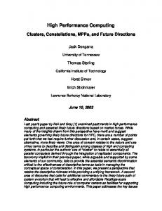
f o r ( i n t i = 0 ; i < C . Length ; i ++) 0000003 e xor edx , edx 0 0 0 0 0 0 4 0 t e s t ebx , ebx 00000042 j l e 0 0 0 0 0 0 3E 0 0 0 0 0 0 4 4 mov e s i , dword p t r [ e d i +4] C[ i ] = A[ i ] ∗ B[ i ] ; 0 0 0 0 0 0 4 7 cmp edx , e s i 00000049 j a e 00000066 0000004b f l d qword p t r [ e d i+edx ∗8+8] 0 0 0 0 0 0 4 f mov eax , dword p t r [ ebp −10h ] 0 0 0 0 0 0 5 2 cmp edx , dword p t r [ eax +4] 00000055 j a e 00000066 0 0 0 0 0 0 5 7 f m u l qword p t r [ eax+edx ∗8+8] 0 0 0 0 0 0 5 b f s t p qword p t r [ e c x+edx ∗8+8] f o r ( i n t i = 0 ; i < C . Length ; i ++) 0000005 f i n c edx 0 0 0 0 0 0 6 0 cmp ebx , edx 00000062 j g 00000047 0 0 0 0 0 0 6 4 jmp 0 0 0 0 0 0 3E 0 0 0 0 0 0 6 6 c a l l 62 D5922C 0000006b int 3

while (pA >= aArr ) { 000000 c5 mov eax , dword p t r [ ebp −10h ] 000000 c8 cmp eax , e s i 000000 ca ja 0 0 0 0 0 0 E8 ∗pC−− = ∗pA−− ∗ ∗pB−−; 000000 cc mov edx , e d i 000000 ce add e d i , 0 FFFFFFF8h 0 0 0 0 0 0 d1 mov ecx , e s i 0 0 0 0 0 0 d3 add e s i , 0 FFFFFFF8h 0 0 0 0 0 0 d6 mov eax , ebx 0 0 0 0 0 0 d8 add ebx , 0 FFFFFFF8h 0 0 0 0 0 0 db fld qword p t r [ e c x ] 0 0 0 0 0 0 dd f m u l qword p t r [ eax ] 000000 d f f s t p qword p t r [ edx ] while (pA >= aArr ) { 000000 e1 mov eax , dword p t r [ ebp −10h ] 000000 e4 cmp eax , e s i 000000 e6 jbe 0 0 0 0 0 0CC 000000 e8 xor edx , edx 000000 ea mov dword p t r [ ebp −18h ] , edx 0 0 0 0 0 0 ed mov dword p t r [ ebp −14h ] , edx 000000 f 0 mov dword p t r [ ebp −10h ] , edx 000000 f 3 jmp 0 0 0 0 0 0 4A 000000 f 8 c a l l 62 F3922C 000000 f d int 3

Figure 2.2.: Two loops over large arrays. On top the C# code is shown. On the left side, the calculation is done the naive way with safe array indexing. The right side performs the same operation with pointer arithmetic. Below, the corresponding (JIT compiler optimized) machine code fragments are shown. Due to acceptable optimizations on the left side, the runtime performance difference is almost negligible. However, the unsafe variant offers much more potential for further optimization control by the developer. Refer to Figure 2.3 for an example.

18


2.5. Performance Design Goals

// u n r o l l e d i n n e r l o o p (C#) double ∗ pA = aArr , pB = bArr , pC = c A r r ; f o r ( i n t i = 0 ; i < l e n − 8 ; i += 8 ) { pC [ 0 ] = pA [ 0 ] ∗ pB [ 0 ] ; pC [ 1 ] = pA [ 1 ] ∗ pB [ 1 ] ; pC [ 2 ] = pA [ 2 ] ∗ pB [ 2 ] ; pC [ 3 ] = pA [ 3 ] ∗ pB [ 3 ] ; pC [ 4 ] = pA [ 4 ] ∗ pB [ 4 ] ; pC [ 5 ] = pA [ 5 ] ∗ pB [ 5 ] ; pC [ 6 ] = pA [ 6 ] ∗ pB [ 6 ] ; pC [ 7 ] = pA [ 7 ] ∗ pB [ 7 ] ; pA += 8 ; pB += 8 ; pC += 8 ; }

// o p t i m i z e d d i s a s s e m b l y 0000018 e xor esi , esi 00000190 mov edi ,2708 h 00000195 test edi , edi 00000197 jle 0 0 0 0 0 1EE pC [ 0 ] = pA [ 0 ] ∗ pB [ 0 ] ; 00000199 fld qword p t r [ e c x ] 0000019b fmul qword p t r [ edx ] 0000019d fstp qword p t r [ eax ] pC [ 1 ] = pA [ 1 ] ∗ pB [ 1 ] ; 0000019 f fld qword p t r [ e c x +8] 0 0 0 0 0 1 a2 fmul qword p t r [ edx +8] 0 0 0 0 0 1 a5 fstp qword p t r [ eax +8] pC [ 2 ] = pA [ 2 ] ∗ pB [ 2 ] ; 0 0 0 0 0 1 a8 fld qword p t r [ e c x +10h ] 0 0 0 0 0 1 ab fmul qword p t r [ edx+10h ] 000001 ae fstp qword p t r [ eax +10h ] pC [ 3 ] = pA [ 3 ] ∗ pB [ 3 ] ; 0 0 0 0 0 1 b1 fld qword p t r [ e c x +18h ] 0 0 0 0 0 1 b4 fmul qword p t r [ edx+18h ] 0 0 0 0 0 1 b7 fstp qword p t r [ eax +18h ] pC [ 4 ] = pA [ 4 ] ∗ pB [ 4 ] ; 0 0 0 0 0 1 ba fld qword p t r [ e c x +20h ] 0 0 0 0 0 1 bd fmul qword p t r [ edx+20h ] 000001 c0 fstp qword p t r [ eax +20h ] pC [ 5 ] = pA [ 5 ] ∗ pB [ 5 ] ; 000001 c3 fld qword p t r [ e c x +28h ] 000001 c6 fmul qword p t r [ edx+28h ] 000001 c9 fstp qword p t r [ eax +28h ] pC [ 6 ] = pA [ 6 ] ∗ pB [ 6 ] ; 000001 cc fld qword p t r [ e c x +30h ] 000001 c f fmul qword p t r [ edx+30h ] 0 0 0 0 0 1 d2 fstp qword p t r [ eax +30h ] pC [ 7 ] = pA [ 7 ] ∗ pB [ 7 ] ; 0 0 0 0 0 1 d5 fld qword p t r [ e c x +38h ] 0 0 0 0 0 1 d8 fmul qword p t r [ edx+38h ] 0 0 0 0 0 1 db fstp qword p t r [ eax +38h ] pA += 8 ; pB += 8 ; pC += 8 ; 0 0 0 0 0 1 de add ecx , 4 0 h 000001 e1 add edx , 4 0 h 000001 e4 add eax , 4 0 h f o r ( i n t i = 0 ; i < l e n − 8 ; i += 8 ) { 000001 e7 add esi ,8 000001 ea cmp esi , edi 000001 ec jl 00000199

Figure 2.3.: The inner loop from the code example in Figure 2.2 was unrolled. The pointer accesses are reformulated for better optimization by the JIT compiler. The number of overall instructions for all iterations is considerably decreased that way. This version executes at roughly half the time of the version on the right side in Figure 2.2


19

2. Design Goals algebra functions for example is written (and accepted) in FORTRAN. Translations exist for C and several other languages and potentially bring bugs and other nuisances. Using binary packages created out of the original FORTRAN compilation ensures both: speed and reliability. And the existence of native interfaces is yet important for increased flexibility for the user of a numerical library. That way it is possible to incorporate existing custom native solutions or certain custom optimized code into the managed program. With MC++ (managed C++), the .NET platform provides the ability to create mixed execution mode modules: managed and unmanaged program parts are contained within the same module and get linked dynamically at runtime. For .NET applications this method is an outstanding efficient way of implementing and deploying custom extensions to managed applications. Lastly, .NET — due to the unsafe options of the CLR — enables the direct execution of precompiled machine instructions. While being cumbersome for larger algorithms (due to the same reasons why assembly language is seldom utilized for this task) the option represents a potential improvement for very inner computational loops like those found in the inner kernels of GOTO BLAS16 . Next to the utilization of native dynamic linked libraries, it is another option to achieve peak performance — truly ’within’ the CLR.

2.5.3. Parallel execution models Thread level parallelism The option of executing portions of code in parallel on a thread level is one of the key features for a ’real’ GPL. At the same time, most of today’s specialized DSL cannot compete in this area. The existence of fine grained — hence high level — synchronization constructs allows for carefully tuned splits of algorithms for optimal utilization of shared memory by multiple threads. However, at the same time these options require a good knowledge of the underlying nontrivial functioning of the OS and the computer architecture. Since this knowledge is often limited among the intended audience, the library should find a good balance between simplicity and flexibility. Builtin functions should parallelize and adapt to the system configuration automatically. The user, however, is free to fall back to the full spectrum of synchronization options the .NET framework provides if higher flexibility is needed. SIMD Utilization While not being obligatory for feasible computations, the utilization of SIMD principles is necessary in order to catch up to the peak performance of highly optimizing languages like FORTRAN. The absence of support of processor specific SIMD instructions by the JVM among others has been claimed as one big point of conflict during the evolution of the javanumerics project and was obviously one of the major reasons the project was abandoned. By now, Javas HotSpot JIT offers limited support17 for SIMD extensions. 16

Goto, K. and van de Geijn, R. A. 2008. Anatomy of high-performance matrix multiplication. ACM Trans. Math. Softw. 34, 3, Article 12 (May 2008), 25 pages. DOI = 10.1145/1356052.1356053 http://doi.acm.org/10.1145/1356052.1356053 17 (’limited’ — because SIMD utilization is not officially specified and hence out of reliable control by the developer)

20


2.5. Performance Design Goals The .NET CLR is far behind. However, attempts are made by the mono project, which provides the mono.SIMD namespace for the developer to instruct the execution of SIMD processor instructions explicitly. Similar to the JRT, plans for a reliable support of such instruction sets are currently barely visible for the CLR18 . Therefore, in order to utilize SSE extensions on x86 for example, the developer must resort to native linked libraries or utilize the cumbersome support of binding managed delegates to native function pointers. At least, this option exists even if it would hardly reach wide acceptance. Unless the CLR designers in the JIT compiler teams suddenly decide to give the numeric computing community a reasonable importance rating, SIMD instructions are unlikely to increase the speed of numeric algorithms for .NET out of the box any time soon. Luckily, alternatives have appeared: GPU processing is pushed towards scientific computations, mainly by the two major graphics card vendors, NVIDIA19 and AMD20 . While NVIDIA at the first place succeeded in establishing the CUDA21 interface, the OpenCL standard version 1.2 was released on Nov. 15th 2011 by the Khronos Group22 and is likely to get accepted by an even wider audience. One of the last obstacles related to OpenCL is the lack of obligatory support for double precision calculations. By time of writing only 35 % of the NVIDIA graphics cards did provide support for double precision23 without emulation. However, the tendency towards a broader support is visible among new releases. In the meantime, the alternative of emulating double precision exist for the cost of several factors of slower execution speed. OpenCL is not limited to graphic processing. It rather aims towards the support of all processing resources available at runtime including multicore support and SIMD extensions on CPUs. Therefore, at the end of that promising evolution is the hope, that the missing link to CPU SIMD extensions can be closed by the utilization of OpenCL. Unfortunately, while being one of the most promising perspectives for future enhancements, none of the options presented in this section could be implemented in time for this work.

2.5.4. Performance gains by design In the view of the inventors of Java and C#, options for runtime execution performance optimizations on behalf of the developer are mostly restricted to using ’proper’ programming techniques. Indeed, the program design is the major domain which most drastically influences the final program speed. And possibly the most important key to a good design is highly related to the way memory is used. This especially holds true for managed virtual environments. In anticipation of the next section, we claim the following memory related design goals: • Design the storage of data objects (arrays) in a way that enables access to elements 18

http://blogs.msdn.com/b/davidnotario/archive/2005/08/15/451845.aspx http://www.nvidia.com 20 http://www.amd.com 21 http://developer.nvidia.com/category/zone/cuda-zone 22 http://www.khronos.org/opencl/ 23 See: http://developer.nvidia.com/cuda-gpus In order to support double precision, the ’Compute Capability’ must be 1.3 or greater. A similar list is found at http://en.wikipedia.org/wiki/Comparison of AMD graphics processing unit for AMD cards. 19


21

2. Design Goals in the most efficient way. • The storage format for arrays should enable the interconnection between well known native optimized libraries. • Prevent copies of array storage as much as possible. • Limit the number of (re-)allocations for array storage. • Design the memory management in a transparent, robust way. Prevent the user from misusing it. • Provide profiling capabilities to the user that allow for efficient runtime monitoring of the memory footprint produced by the implementation. In the next sections we’ll give a short overview of the memory management of the Common Language Runtime. The memory design presented in Chapter 4 is derived from these insights.

2.6. CLR Memory Management This section gives an overview of the inner functioning of the memory management in the CLR. Most principles mentioned here can be similarly found on the Java platform. Both utilize a generational, compacting garbage collector24 . Java — in contrast to the .NET CLR GC — provides a full range of configuration options 25 to the user. The concept of a Large Object Heap seems almost unique26 to the .NET CLR. Knowing the details of the underlying runtime architecture helps the design significantly. Implementers of similar projects for the Java platform are advised to study the technical references; some good starting points were given here already. .NET memory management relies on a generational, compacting garbage collector. The main advantage of using a garbage collector over the classical C/C++ approach is, that the developer is technically disabled from producing memory leaks27 by mistake. Languages for such environments do only provide the possibility to allocate — but not to free resources deterministically. The de-allocation is done automatically by the runtime. Therefore, further unused objects are collected from time to time and their memory area is ’freed’ for consecutive reallocation. However, it is still possible to produce ’unhealthy’ large memory consumption, if large objects are kept on being referenced from any root object on the stack. And — as we will see — while somehow releasing the developer from the attention of preventing from serious bugs, this technique brings important implications in terms of performance for resource intensive applications. 24

Java GC FAQ: http://www.oracle.com/technetwork/java/faq-140837.html Technical insight into the architecture of the JVM GC variants and tuning options: http://java.sun.com/javase/technologies/hotspot/gc/gc tuning 6.html and http://www.artima.com/insidejvm/ed2/gcP.html 26 with the exception of the Oracle JRocket VM, see http://en.wikipedia.org/wiki/Jrockit 27 A ’leak’ is considered an allocated area of memory to which any reference was lost, hence cannot be freed anymore.

25

22


2.6. CLR Memory Management

2.6.1. Managed Heap and Generational GC In this section we will give an overview of the functioning of the .NET managed heap. We will concentrate on those features which are most important for our purpose. More detailed articles exist28 29 for the interested reader. In a simplified view, the .NET runtime can be seen just as a regular (native, unmanaged) program or service. It loads byte code compiled programs (so called assemblies), inspects their meta data, prepares an execution environment (so called application domain) and starts executing them. For the assembly, the hosting runtime environment appears like an operating system30 . An assembly requests memory from its environment in form of types. Since C# is a strong typed language, when we are talking of ’memory’ from the C# point of view — we are actually mostly talking of types. In C#, such types commonly are created by the keyword new. How does the runtime deliver memory for allocation requests? The CLR allocates memory from the virtual memory address space by using the memory manager of the operating system. Memory is delivered in segments 31 . From the perspective of virtual memory, the managed heap is built out of several chunks and those chunks are not necessarily sequentially arranged in memory. Initially, the runtime allocates two chunks, one for the allocation of small objects (a so called small object heap segment) and another one for the allocation of large objects (large object heap — LOH ).

2.6.2. Small Object Heap Once the memory segments for the managed heap are reserved, the runtime may start registering memory areas for types of them. The small object heap is organized in generations. Currently, the .NET CLR uses 3 generations: ephemeral generations 0 and 1 and the generation 2, where longer living objects are hold. A generation is defined by its addresses for starting and ending range only. Those limits of a generation may frequently change during regular runtime service support procedures (i.e. garbage collection). Figure 2.4 demonstrates the basic principle of the GC in the small object heap. Initially, in a new segment the whole space is defined as generation 0. New allocations are done from that generation. If memory for a new object is requested, the current allocation pointer value marks the beginning for the new memory region. The allocation pointer is simply increased by the needed length for the new object. Therefore, successful allocations from the managed heap are fast. Particularly such allocations are cheaper than those from the regular (virtual) memory manager, commonly used for example in C++. As soon as the allocation pointer reaches the end of the ephemeral segment, a garbage collection is triggered in order to clean up unused objects and make room for further allocations. The garbage collection is done by first considering all objects as garbage and afterwards subsequently walking live objects, marking them for survival. This will create ’holes’ in the heap. In the compacting step, those holes are filled by 28

Garbage Collection insights, Part1: http://msdn.microsoft.com/de-de/magazine/bb985010%28enus%29.aspx 29 Weblogs of the chief of the CLR GC team, Maoni: http://blogs.msdn.com/b/maoni/ 30 This is the reason for the naming: ’virtual runtime environment’ — a virtual environment, which only exists as software program and is executed within a hosting environment itself. 31 The segment size is 16 MB at minimum for a 32 bit process. The number for 64 bit is not published but experiments show that it lays several factors higher.


23

2. Design Goals

Figure 2.4.: The ephemeral segment of the managed heap. The empty segment (a) is filled with allocated objects. Once there is no more space left for the new object 5 (seen at b), non garbage objects (1 and 4) are collected, compacted and promoted to generation 1. The end of generation 1 marks the new beginning for generation 0 and consecutive allocations (c). moving survived objects until all holes are closed. At the end of a collection cycle, all survived objects are moved to the bottom of the ephemeral segment and the generation limits are adjusted accordingly. Generation 1 now includes the survived objects. Generation 0 will start at the end of the last object survived. If there is still not enough space available for the new allocation request after a collection of generation 0, the process is repeated for generation 1 objects and even for generation 2 if necessary. Because the limits of every generation are always well known, the collector is able to restrict a collection to only those objects, which exist in a specific generation. Therefore, by limiting a garbage collection to objects in generation 0 or 1, the cleanup for ’young and short lived’ objects is relatively fast. A full collection on the other hand (i.e. including all generations) can be expensive and time consuming since the full tree of application objects needs to be investigated. In an optimal scenario, the collector would be running rather frequently on the young generations 0 and — at most — 1. Full generation 2 collections should be rare. If the software design is able to support that scheme, it ensures a high memory management performance. It must be noted that the process described here is more complex in reality due to the existence of finalizable objects, weak references and pinned small objects. However, since the best performance can be achieved by preventing or limiting the use of such features, we will not rely on them and hence do not have to consider them here in more detail.

2.6.3. Large Object Heap In general, memory segments requested from the systems virtual memory to be used as managed heap segments are 16MB in size32 . Such segments are destined to host 32

The limit is valid for 32 bit processes in the .NET CLR. The value for 64 bit systems is not published by Microsoft. In experiments it appeared to be 128 MB for the LOH, 256 MB for the ephemeral

24


2.6. CLR Memory Management small objects like class instances, string objects and small arrays. Due to its compacting nature of the heap, the limited size of these segments and the fact they — once empty — are released to the operating system memory manager immediately, the heap is able to adapt quickly to changing memory needs of the application and at the same time preserving good memory locality. This is true for common business case scenarios on most real world applications. However, larger objects are handled in a different manner. Above a certain limit, LOH segments serve the memory for such objects. For performance reasons the LOH saves the compacting step in a garbage collection. Holes may be created by released large objects, threaded into a free-list and considered for subsequent allocations. That is why such allocations are more expensive. Extremely large objects are rare for common business scenarios33 . However, for our concerns, they are the base of most numerical objects. The current CLR implementation34 considers the following objects as ’large’: • Objects of at least 85.000 byte in size. • System.Arrays of element type double and length 1.000 or more. • Some support object structures, which the environment uses (and are not further considered here). Double arrays of 1000 elements can be found to be a rather common case for scientific applications. In conjunction with the fact that all garbage collections on the large object heap are expensive generation 2 collections, evidently precautions against frequent allocations from the LOH are necessary.

2.6.4. Heap Fragmentation There is another threat endeavouring such precautions. Dynamic memory is prone to heap fragmentation issues for certain allocation patterns. This is true for both, managed heaps and those heaps managed by the operating system virtual memory manager. Consider a situation where fragmentation on the managed heap may occur: An application allocates large sized arrays of different length in a loop. If some of the smaller sized arrays have a longer live time than others, this may lead to a fragmentation scenario. As a result, the memory is not efficiently used and allocation requests may get refused with an OutOfMemoryException. Figure 2.5 points out one possible scenario. Note that the fragmentation of the managed heap is unlikely to be caused by those objects which exceed the minimum segment allocation size (16 MB on 32 Bit). Larger arrays trigger a whole segment on their own. Releasing such objects likely causes the segment to be returned to the OS. The CLR allocates such huge segments with size of multiples of 8 MB (128 MB on 64 bit processes35 ) or with lengths of power of two for middle sized heap. Note that most ’large’ objects are assembled out of several smaller objects itself. One example is a large data structure for a business object holding all user data. The largest independent memory area used by such a structure would be the largest individual (atomic) entity used by the class. 34 As due .NET 4.0 35 The numbers for 64 bit processes are not published by Microsoft and are result of experimental investigations. 33


25

2. Design Goals

Figure 2.5.: Fragmentation on the Large Object Heap. On the left side, three segments are shown which were filled up with larger and middle sized objects. One extremely large object of 160 MB covers a whole segment alone. After a GC collection (right) the three largest objects are released. However, since some smaller objects survived, two segments cannot get released to the OS. They stay reserved, waiting for matching allocation requests and fragmenting the heap. However, the segment for the largest object is now empty and therefore returned to the OS or used for the current allocation request. LOH objects. Therefore a chance exists for a rather ”middle sized large object” to cover the space above the allocated huge object. The chance on 64 bits apparently is larger. A similar fragmentation may occur on the virtual memory (VM). This is caused by repeated disadvantageous allocation requests to the VM manager. Say, large managed heap segments of varying sizes are requested repeatedly. Some of them are returned and some are kept reserved. Holes opened by the freed blocks can only partially get reused by subsequent requests. This might be caused by new arrays which are even a little larger in size or the virtual adress space being partially obscured by other runtime requests in the meantime. Therefore, the virtual memory space would get fragmented with holes similar to the managed heap segment scenario. It must be emphasized that fragmentation basically is not a problem of CLR or virtual environments in general. The functioning of the large object heap is comparable to that of the regular virtual memory managed heap. Every application handling potentially extremely large objects must keep track of that fragmentation issue. There is not much a developer can do against such nuissances next to preventing from those allocation patterns. The best help here is to use a pool for such large objects and reuse them whenever possible. The following options may be used in conjunction to that: • Deterministic disposal: further unused objects should be freed and their memory returned as soon as possible — at best immediately. This contradicts to the main principle of ’managed’ memory management but is crucial for a fast and stable memory allocation mechanism. Several (scripting) languages like (again) numpy and MATLAB utilize interpreters36 to achieve this goal. R

36

python uses reference counting to clean up unused objects from its internal heap. A garbage collector

26


2.6. CLR Memory Management • On Windows up from Server 2003, local heaps created for applications are configured as ’Low Fragmentation Heaps (LFH)’37 per default. This helps decreasing memory fragmentation caused by smaller type sizes (< 16kB). In general, as stated above, every allocation pattern requesting and freeing memory in a subsequent manner is sensible for fragmentation. The only way to avoid heap fragmentation reliable and feasible is to avoid frequent allocations.

2.6.5. Memory Management Conclusions As seen in this section, frequent allocations of large objects introduce serious disadvantages like heap fragmentation and memory displacement. In addition, allocations from the LOH are more expensive than from the top of generation 0. For huge arrays, a new even adds about the same effort than for unmanaged environments to the managed costs since a full new segment often has to be requested from the memory manager of the OS. Last but not least, such frequent allocations cause the working set to spread over a much larger area of virtual memory, badly decreasing the locality of the data which in turn causes much more page- and cache misses and hence less efficient data caching. The vendors of virtual environments invest large efforts to handle frequent allocation requests. Especially for large objects, alternative GC strategies are utilized38 . They may prevent exceeded memory usage and work against some of the problems described above. However, the computational effort is relatively large. For .NET a configuration for an ’High Troughput GC’ could easily cause the application to spend half the execution time in GC only — time which is better used for profitable computations. The lesson learned from these considerations is: for high throughput computations, large arrays should not be fully released but somehow reused. This will be the main performance goal for our implementation in the next chapter. In Section 4 the implementation of an efficient memory management is elaborated. In Appendix A.3 a comparison is made which demonstrates the obvious effect of frequent allocation patterns to memory fragmentation and the success of reallocation prevention by memory pooling.

is used to detect and remove cyclic references only, which reference counting is unable to handle. http://msdn.microsoft.com/en-us/library/aa366750.aspx and http://illmatics.com/Understanding– the– LFH.pdf 38 Several variants of the JVM handle large objects differently. The concept of a large object heap is somehow similar found by the Oracle JRocket VM. Other JVM compact large objects together with smaller ones — a method which is expected to lead to less GC efficiency for large objects. See: http://blog.dynatrace.com/2011/05/11/how-garbage-collection-differs-in-the-three-big-jvms

37


27

3. Implementation In this chapter, a software design for a numerical library for C# is evolved from the requirement considerations gathered in the last sections. The main goals which were focused on were the execution performance (in terms of memory usage and execution speed) and the syntax elements which at the end are important to gain acceptance among the scientific community. The implementation demonstrated here is based on a former open source project named ILNumerics1 .

3.1. Overall Architecture ILNumerics serves three main areas: 1. N-dimensional, generic array objects to be used all over the library. The arrays provide automatic memory management, build lazy, shallow copies via reference counting and support all features common for MATLAB arrays for compatibility reasons. The class design is well prepared for the extension of existing dense arrays to sparse arrays and other special array shapes. R

2. Collection of static builtin functions and higher level algorithms. All functions are found at one place for simplicity reasons and utilize the n-dimensional array objects of the library. Standard low-level functionalities such as FFT and LAPACK functions are encapsulated into interface definitions, for which default native implementations are provided in form of the Intel Math Kernel Library. 3. Visualization classes for data plotting in 2D and 3D. The controls base on standard .NET Windows.Forms controls and therefore are easily utilizable within any .NET GUI application. This work focuses on the first part.

3.2. Storage This section describes the main storage format for the most important numeric array objects.

3.2.1. Element Storage For the design of tensor objects, syntax requirements as well as performance consideration have to be taken into account. C# provides n-dimensional array objects out of the 1

See the official website of the project: http://ilnumerics.net. The libraries offered here are provided under a commercial license since Nov. 2011.


29

3. Implementation

Figure 3.1.: The building blocks of ILNumerics. box. Unfortunately, those arrays lack many required features like subarray read/write access, compatibility with native libraries and an efficient implementation. Therefore, standard one-dimensional arrays will be used as a base storage for all n-dimensional arrays. Wrapper classes isolate low-level, element based access from higher level usage and provide the API corresponding to the syntax requirements.

3.2.2. Wrapper Class Design The array wrapper classes use the generic capabilities of C#. That way, their use is not limited to numeric element types. Just as well, such arrays are usable with custom base classes or custom structs. One example could be a modified implementation of complex numbers or of arbitrary container classes which can be arranged in a multilinear manner that way. For an efficient syntax it is profitable to provide a non-generic base class. Furthermore, the implementation is not sealed. Future updates may bring other matrix implementations besides the currently implemented dense arrays. One example would be sparse arrays. Therefore, ILBaseArray serves as the abstract general base class for all arrays. The only specialization provided for now is the abstract ILDenseArray — a general purpose dense array of arbitrary element type. However, the user does only handle concrete implementations of that dense array, mostly: ILArray. Two further concrete array types exist: ILLogical and ILCell. Both serve special requirements for special element types: ILLogical can be seen as a boolean tensor and is often needed in conjunction with logical operations. ILCell provides a comfortable way of handling arrays of other arbitrarily sized and typed arrays. Other concrete array

30


3.2. Storage

Figure 3.2.: Class Diagram of all array related bases classes. The left tree marks the layer for memory management; the right tree shows the main classes for the storage layer.


31

3. Implementation

Figure 3.3.: Wrapper classes for array element storage implementations exist, which are needed for memory management only. Their use is described in Section 4.3.1 and is restricted to very few rules in order to achieve perfect memory efficiency. The underlying System.Array for array element storage is wrapped into several classes according to Figure 3.3. The design supports fast shallow clones with lazy data copies on write access, altering of subarrays, partial removal and expanding of subarrays at runtime, performant reshapes and efficient memory pooling.

3.2.3. Subarray access, Expressions In the last section, one example for subarray access has been presented already. The options for subarray access are very extensive and will only partly discussed here. In fact, subarray access is fully compatible to the subarray feature in MATLAB . Therefore, we only give an overview of the syntactical differences between both languages in Table 3.1. R

3.2.4. Array Interaction and Mutability Rules The most important mathematical operators are overloaded for all array types: +, −, /, ∗, , |, &, ! = and ==. All operators expect arrays of the same size on both sides. Alternatively, one of the arrays may be a scalar in which case the operation uses the scalar value for all elements of the other array respectively. Vector sized arrays are allowed to operate on matrix sized arrays elementwise once their shape matches either rows or columns of the matrix.

32


3.2. Storage Once a local array is created, it can be altered only by few operations. Examples are the SetValue() and SetRange() functions as well as left side index access. Here the same subarray syntax can be used as for read access (indexing on the right side) on assignments. Example: ILArray A = z e r o s ( 5 , 4 ) ; A[ end , 0 ] = 1 ; // a l t e r t h e l a s t // A [ 5 , 4 ] [0]: 0 0 [1]: 0 0 [2]: 0 0 [3]: 0 0 [4]: 1 0

e l e m e n t o f column 0

0 0 0 0 0

0 0 0 0 0

A[ 1 , 5 ] = 5 ; // expands t h e a r r a y t o t h e 6 th column A[ end −1, f u l l ] = n u l l ; // removes t h e f o r e l a s t row // A [ 4 , 6 ] [0]: 0 0 0 0 0 [1]: 0 0 0 0 0 [2]: 0 0 0 0 0 [3]: 1 0 0 0 0

R

0 5 0 0

MATLAB Subarray

ILNumerics Subarray

a(5) (parenthesis,

a[4] (bracket use,

1 based indexing)

0 based indexing)

Addressing full dimensions

a(1, :)

a[0, f ull]

Addressing ranges

a(1 : b, 2 : 2 : end)

a[r(0, b),r(1, 2, end)]

a(:, end/2)

a[f ull, end/2]

Linear indexing

a(b)

a[b]

Arbitrary indices

a([1, 2, 1], [2, 2, 3])

Conditional indexing

a(a < 5)

General index access

Addressing relative to last element

Optional output

[Q, B] = qr(A)

parameter suppression

[Q, ∼] = qr(A)

Vector - Matrix

A − repmat(M, 1, n)

binary operation

bsxf un(@minus, A, M )

a[cell(0, 1, 0),cell(1, 1, 2)] or a[”0, 1, 0; 1, 1, 2”] a[a < 5] Q = qr(A, B); Q = qr(A) A−M

Table 3.1.: Array handling in MATLAB and ILNumerics. The table demonstrates the similarities and differences of array handling in both frameworks.


33

3. Implementation Mutability of arrays plays an even larger role in the memory management of ILNumerics which will be discussed in Section 4.

3.3. Miscellaneous Features A number of builtin functions have been implemented. The collection provides common functionality for numerical arrays. It spans the area of fundamental array manipulations, basic linear algebra functions like matrix decompositions, a collection of efficient sorting routines and functions for fast fourier transforms. The design of those functions is similar to the well known and established elmat functionality of Wothworks’ MATLAB . R

3.3.1. Parallelization All builtin functions are capable of automatically parallelizing the execution on larger arrays for systems with more then one processor core. However, the .NET framework does provide several options for simplified parallel execution models itself. In order to enable the use of these framework functions, the number of parallel executing threads is configurable by the user. Just like for memory usage, some considerations must be taken into account for a threading model. Number of Threads and Contention The .NET Framework provides an efficient implementation of a thread pool. Its use limits the overhead of creating new threads for parallel tasks by reusing existing threads from the pool. Up from .NET 4.0, the Task Parallel Library does even simplify the parallel execution of so called Tasks which are arbitrary program segments. However, the scheme is optimized for relatively long running task items. It internally makes use of the .NET thread pool which in turn configures itself automatically. This affects the number of parallel running threads and the number of parallel queued task items. The optimizations and default configuration obviously targets common business scenarios. So, the standard implementation automatically manages the number of active threads in the thread pool as the quantity of queued task items changes. Many applications profit from technologies like simultaneous multithreading (SMT)2 . However, numerical calculations bring slightly different requirements than common business software. Those applications commonly handle arrays of numeric element type and calculate numbers from its elements. The most time in these algorithms is spent on copying data within processor caches and by utilizing the FPU. It is obvious that SMT is less profitable in those situations and eventually even slow down the processing3 . In addition, the task items for such calculations are relatively small in execution length but for them, it is crucial to start very fast and so to signal its completion to the main thread. Synchronisation between the threads can get done fastest by using spin locks. The standard thread pool implementation on the other hand appears to be overkill and less efficient here, since it uses Thread.Sleep() for synchronization — which in our 2 3

A well known representative of SMT is Intels Hyper Threading Technology. Even Intel recommends disabling SMT for such purposes and for its own products: http://software.intel.com/en-us/articles/setting-thread-affinity-on-smt-or-ht-enabled-systems

34


3.3. Miscellaneous Features case increase contention due to inefficient context switches. Also, it implements several feedback and cancellation mechanisms which are not needed here. Therefore, a custom thread pool has been implemented. It provides the exact fixed number of additional threads needed. Only the number of physical cores has to be taken into account4 . Those threads are steady running next to the main thread. Similar to a common thread pool scheme, new work items are queued into a pending tasks queue — for each thread separately. This not only saves the management overhead for assigning tasks to the available threads but also limits potential context switches between processor cores. In addition, a lower limit on the number of elements of corresponding data for every function class is introduced. The limit determines up from which data size the function is executed in parallel. This prevents the calculation of very small data to be slowed down due to parallelization overhead. The limit is distinct to classes of functions according to their complexity. The following table shows the default values for these limits. Complexity Class

Default Parallel Limit

Example

O(n)

2000

sin(), abs(), add()

O(n2 )

1000

sort()

O(n3 )

250

matrix multiplication

These default limits are empirically determined. A more efficient (and possibly even faster) system could iterate these values (and other configuration values in the library) at application startup and find the optimal configuration for the current system setup.

4

Unfortunately, there currently is no reliable way of determining the number of physical cores on a Windows system via .NET. On hyperthreaded processors for example, the number of cores reported will reflect the number of virtual cores — i.e. the physical cores plus any virtual (HT) cores for them. Therefore, the number of threads is set in the configuration file.


35

4. Memory Management ILNumerics implements a memory management based on strongly typed array wrapper classes. Implicit type conversions, deterministic disposal and a fast memory pool implementation are the main building blocks here. Those components are explained in the following chapter in greater detail.

4.1. Memory Management Overview The main idea behind the ILNumerics memory management is the automatic reuse of large storage objects. Most long running algorithms utilize data of similar sizes inside computational loops. The expectation therefore is that in most cases the allocation pattern of such loops exhibits some kind of periodic structure which makes using a pool feasible. Figure 4.1 gives an overview of the main components involved. The next section explains some details about the inner functioning of the memory pool. Both, the reallocation from pool and the returning of no longer used storages back to the pool introduce some serious problems. Those are addressed in Section 4.4.

4.2. Memory Pool The goal of the memory management is to achieve perfect reusing of all array storages. Therefore one dimensional system arrays — used as bottom most storage objects — are collected in the ILNumerics memory pool for subsequent allocation requests. Only if no matching storage was found in the pool, a new storage is allocated via the CLR — i.e. from the systems virtual address space. However, for practical situations it is unlikely that recurring array storages all have the same size. Consider the common kmeans algorithm in Appendix A.2 as one example. The main computational loop selects matching data points in every iteration over the clusters. According to the number of matching points found the sizes of the arrays created here change frequently. It would be unlikely to find matching storage sizes in the pool for all such cases. This is — of course — also true for situations where random array sizes come into play. How does the ILNumerics memory pool handle these problems? By ’matching storage’ every storage size is considered which is at least as long as the size requested. A certain parameter exists in the pool which introduces an upper limit for matching sizes. As a consequence, arrays in ILNumerics may use underlying storage objects which may be larger in size than the number of elements shown to the user of the array. Since the common array API encapsulates the inner storage nearly completely, this behaviour is transparent to the user. The implementation stores all existing storages in a dictionary data structure — for O(1) direct access. In addition, an index of the storage sizes is created with a custom AVL tree implementation. It is used to query the pool for the next larger storage size in case the exact size was not found. A successful allocation request


37

4. Memory Management

Figure 4.1.: Overview of ILNumerics memory management. All requests are made from the memory pool. The scoping layer consists of all array classes which are exposed to the user. The actual storage lives in the storage layer which is wrapped within scoping objects.

38


4.3. Usage Rules from the ILNumerics memory pool therefore introduces a cost of at most O(log n), where n is the number of distinct storage sizes currently held in the pool. The ILNumerics memory pool introduces some self-tuning capabilities which optimize the matching search for specific storage lengths. Since in general all dead storages are stored in the pool, optimizing the matching behaviour is not only important in order to prevent for new virtual memory requests but also for preventing an ever growing pool size. Therefore, a dynamic pool optimization continuously collects statistics about the memory requirements of the current algorithm and adapts the pool parameter dynamically towards a small overall pool size and a large reallocation success rate. In detail, the parameters are: • The preferred maximum pool size • The matching length factor • The minimum length from which storages are pooled at all • A proactive allocation lengthening factor which in advance allocates larger storages than needed in case of VM allocations The allocation statistics are tracked continuously. Pool parameters however are only recalculated in certain edge cases like an OutOfMemoryException being thrown or the pool reaching its preferred maximum pool size. Tests have shown that the pool implementation is able to adapt very quickly to real world algorithms up to a reallocation success rate of (nearly) 100%. Even for the worst case scenario of completely random allocation patterns of sizes in the range from some small 1000 double elements to ”large” storage sizes (above 100 MB) and reasonable pool sizes (200. . . 500 MB) the pool achieves permanent success rates clearly above 90%. In Figure A.1 on page 49 in the appendix, an UML diagram of the memory pools ’Request’ activity is given.

4.3. Usage Rules The memory pool is able to efficiently select proper storages out of the collection of pooled storages and uses them for incoming memory requests. However, in order to find matching storages, the library must ensure to immediately return all storages of those arrays to the pool which run out of scope. The garbage collection strategy of .NET somehow contradicts this requirement. Therefore, ILNumerics introduces a custom scoping mechanism. In conjunction with the array typing in the memory management layer, a full deterministic disposal is achieved. The user has to take the following three rules for efficient memory usage into account.

4.3.1. Usage Rule I — Array Type Declarations Function declarations must declare • the return parameter as of type ILRetArray and • any input parameters as of type ILInArray and


39

4. Memory Management • any additional output parameters as of type ILOutArray. Output parameters are always optional. It is recommended to use the C# optional parameter feature. The function should expect the parameter to be null on input. Only if the parameter is not null, an output value should be assigned to it. In the statements above, T is any concrete type. However, those type declarations do only effect the parameter type definitions in the function declaration. Any local variable created in the body of the function must be of type ILArray. An example of a function declaration for a function named myFunc with two input parameters, one additional output parameter and one return parameter in double precision therefore may look as follows: ILRetArray myFunc ( ILInArray A, ILInArray B, ILOutArray outC = null ) { ILArray l o c a l V a r 1 = empty ( ) ; l o c a l V a r 1 = s o r t ( abs (A) ) + B ; return l o c a l V a r 1 ∗ 2 ; } For cell arrays and logical arrays, corresponding array types exist. They can equivalently be used as replacement for ILArray, ILInArray, ILRetArray and ILOutArray in the statements above.

4.3.2. Usage Rule II — Artificial Scoping The body of every function block must be enclosed with the following C# using construct: u s i n g ( ILScope . Enter (A, B) ) { // f u n c t i o n body } using () blocks are a shortcut in C# to create a try/catch/finally block. This is equivalent to writing: IDisposable scope ; try { s c o p e = ILScope . Enter (A, B ) ; // f u n c t i o n body } catch ( ) {} } finally { i f ( s c o p e != null ) scope . Dispose ( ) ; } So, regardless how the function body is left (by regular return or due to an error condition) the artificial scope created by the using block will get disposed. As arguments for the ILScope.Enter() function, all input parameters of the function must be given, i.e. all parameters of type ILInArray. If any other parameter (like output parameters)

40


4.3. Usage Rules are given to the ILScope.Enter() function, no harm will result and they are silently ignored. A scoping block ensures the following contract: after leaving such a block, the memory used by all arrays created during the execution of the block will be released — with the exception of any return parameters of course. To roughly name it another way: the memory used up by arrays will be the same before and after the block. Artificial scoping blocks are not limited to a specific use inside a function. It is allowed to nest scoping blocks. Also, the use of such constructs inside the body of looping statements can help to reduce the overall memory footprint of an algorithm.

4.3.3. Usage Rule III — Function Parameter Assignments In order to assign a value to a variable which was declared as input or output parameter of the function, the property ILInArray.a and ILOutArray.a must be used on the left side of the assignment: outC . a = rand ( 1 0 0 , 1 0 0 ) ; The use of the .a property for the assignment to local variables (i.e. variables of type ILArray) is optional and does potentially further decrease the memory footprint of the algorithm.

4.3.4. Usage Rule Example By blindly following these simple rules, the developer does not need to track any memory disposition or think about reference semantics for the arrays. An example of a (nonsense) computational function: ILRetArray funcName ( ILInArray A, ILInArray B, ILOutArray outC ) { u s i n g ( ILScope . Enter (A, B) ) { // h e r e s t a r t s t h e r e g u l a r a l g o r i t h m d e f i n i t i o n ILArray l o c a l V a r 1 = empty ( ) ; // do s o m e t h i n g h e r e w i t h l o c a l V a r 1 or o t h e r v a r s l o c a l V a r 1 = s o r t ( abs (A) ) + B ; i f ( ! i s n u l l ( outC ) ) { // o u t p u t parameter outC was r e q u e s t e d outC . a = rand ( 1 0 0 , 1 0 0 ) ; } // r e t u r n , no c a s t i n g needed return l o c a l V a r 1 ∗ 2 ; } } The next sections will examine some background of that usage scheme.


41

4. Memory Management

4.4. Scoping and Deterministic Disposal Deterministic disposal is the inherent ability to free resources at a specific (deterministic) point in time. For languages like C++, classes commonly utilize a destructor into which all cleanup code belongs. Virtual language environments often use a garbage collector. C# however (Java as well) knows the concepts of finalization methods anyway. Here, the GC calls a special member function of the class right before the class is cleaned up. For several reasons, finalization schemes are considered bad practice1 and should be avoided. However, it would still be valuable to know immediately when an object is to be freed. Consider an example of a computation with matrices B and C: A = sum ( abs ( s i n (B/128 ∗ p i ) + c o s (C/128 ∗ 2 ∗ p i ) ) ) ; In the naive approach, every operation involved would cause the creation and returning of a new array. All together that line would create 10 arrays of the size max( s i z e (B) , s i z e (C ) ) . As soon as larger arrays come into play, the overhead of having ten temporary objects which are never referenced again just to compute one single output is not negligible. How can we improve this situation? All operations in the above line create arrays which are used as input parameters — exactly one time. The only exception is the return value from the outermost function sum. This return value is assigned to a local variable A and hence may be used multiple times in consecutive algorithm parts. We state the following assumptions: A return value from any function is considered to be a temporary array and used only once. Local variables are expected to be used multiple times. So we already identified two distinct array classes regarding its lifetime: temporary arrays and local or regular arrays. The class distinction is done on the basis of the expected lifetime of the underlying data. But where and how is the disposal happening? In an optimal scenario, every temporary object should get disposed after the first use. There are only very few cases, where an array can be used at all: 1. As input parameter for a function call 2. As source (right side) of an assignment 3. As return value of a function 4. As object exposing properties and / or member functions If we handle to dispose temporary objects in these situations, we get an immediate deterministic disposal and hence efficient memory reuse. In the following subsections all these cases are subsequently solved. 1

Reasons: delayed memory release (2 GC cycles necessary), resurrection complicates the lifetime of objects, the time of disposal is still not deterministic, multithreading issues.

42


4.4. Scoping and Deterministic Disposal

4.4.1. Input Parameter Handling Let’s recall the above example: A = sum ( abs ( s i n (B/128 + p i ) + c o s (C/128 ∗ 2 ∗ p i ) ) ) ; The division operator internally calls the function divide. The function receives B (a local array) and the temporary array which was created from the constant 128. It creates a new storage with the result of B/128. That array is — once returned from divide — fetched into plus. The input of plus therefore are two temporary arrays. According to our assumption, temporary arrays should be disposed after the first use. The first use in this case is the whole function scope where the array was given to (here: plus). Hence, we evolve the next assumption: Functions should release incoming arrays after use, as far as the array is a temporary one and the current scope is the first scope for the array. The last part of the assumption is important, because a function may utilizes incoming arrays multiple times — regardless if it is originated from a temporary array or not. It may even pass the array to another function and expect it to still exist afterwards. In other words, the lifetime of an array is to be extended if it was passed to a new function scope2 . After the plus operator has finished, its return value is given to sin: A = sum ( abs ( s i n (B/128 + p i ) + c o s (C/128 ∗ 2 ∗ p i ) ) ) ; Clearly the input of sin will be a temporary array and can be disposed after sin used it for its calculations. But even more can be done! Since sin ’knows’ of its incoming parameter to be soon disposed, it can do its computations inplace on the memory of the incoming array. That way, no memory must be fetched from the pool and the incoming array does not have to be disposed — it simply gives away its storage to the current function scope.

4.4.2. Assignment Handling Temporary variables are used only once in the creating scope. Local variables are persistent variables. By assigning a temporary array to a local variable, the array must get converted from a temporary array to a persistent one. Here, the C# implicit conversion operators come in handy. It takes the storage of the temporary array and transfers it to a new local persistent array. Now, since we are targeting deterministic disposal, where will that new local array get disposed? One possible way is to dispose it manually by using the Dispose() function, belonging to all array types. But since a robust memory management should prevent the user from having to track array memory at all, another solution is needed. The lifetime of a local array is the local declaration scope3 . The arrays’ memory should be released once the scope is left. Therefore, in Section 4.3.2 we declared a rule 2

We could have defined the last assumption in another way: Temporary arrays are handled as local variables inside callees. Unfortunately, there is no known way of implementing that solution — at least not in C#. We can detect the end of a function (by utilizing the ’using’ keywords), but we cannot detect the returning from a function within the calling scope. 3 Local class members are an exception which is not handled here.


43

4. Memory Management of manual function scoping utilizing using blocks. Such blocks declare an artificial scope. A thread specific scope stack is created around the function body. As soon as the block is left (no matter where and how), the current scope block is signalled to clean up all local variables created during its lifetime. Input parameters on the other side are considered immutable. This means that arrays pointed to by those parameters cannot get altered. Immutability is ensured by class design (input parameter arrays do not provide any public method to change their elements nor their shape) and needed to realize value type semantics for all function parameters. Technically there is no way to prevent a user from reassigning an array to any existing input parameter variable. By doing so, the original array given to the input parameter on function call is not altered and the requirement of a value semantic still holds. However, because the assignment would diminish several execution speed optimization options, the framework by definition prohibits assignments to input parameters completely. The author considers this rule as a nuisance that can be minimized by the fact that assignments to in/output parameters in an algorithm are mostly needed in the context of input parameter checking and the returning of algorithm results — i.e. at the beginning and the end of an algorithm. Input parameter assignments may even be seen as bad practice at all so it is recommended to abstain from them anyway.

4.4.3. Return Value Handling Returning an array is simple; by convention (see Section 4.3.1) all functions return temporary arrays of type ILRetArray/ ILTempCell or ILTempLogical. The output of another function is simply returned without change4 . In order to be able to return local array variables as well, implicit conversion operators exist which transform any array type into ILRetArray implicitly. The conversion is done by creating a shallow, lazy clone of the original array.

4.4.4. Handling Object Member Calls The last usage case for temporary arrays is the employment of its public API. Consider the following example: i n t l = f i n d (A > B ) . Length The temporary array returned from find, should be released after using its Length member. Therefore: Temporary arrays must dispose themselve after any member invocations.

4.4.5. Holes in the Scheme The artificial scoping implementation presented here is not waterproof. For example, the statement tan(A); creates a temporary object which is only cleaned up by the garbage collector — at least. However, the statement does not produce any side effects either 4

Exactly spoken, this conflicts with the only-one-usage-rule for temporary arrays. However, for simplicity we hereby define the returning of an object of the same type as the return type not to be a ’usage’ but only the copy of its reference address on the stack knowing, that afterwards the original copy will not exist anymore since we just left the function scope and the stack gets cleared.

44


4.5. Value Type Semantics and therefore is considered nonsense. The design of the memory management does only catch those cases where arrays are involved into a usefull calculation. All other cases (including the intention to trick the memory management by creating arrays without actually using them) will eventually not profit from the improvements introduced here. However, computational correctness is still guaranteed.

4.5. Value Type Semantics One of the requirements left out so far is the common expectation of scientists to get value type semantics for function parameters. Input variables in functions are expected to act like local variables and callers of functions expect the function not to change the original array in the callers scope — unless explicitly stated. Even if C# passes parameters by reference, a similar behaviour is achieved by the definition of two new array types: ILInArray and ILOutArray (see Section 4.3). Both types can only be constructed by use of implicit conversion operators from other array types. By passing an array of type ILRetArray to a function expecting an input parameter of type ILInArray, the temporary array gets converted to a (persistent) input array. This does not introduce any data copies (not even a lazy one) since the function call will be the only use of the temporary array. The input array itself is registered for disposal in the opening artificial scope, obligatory by convention for every function body (again see Section 4.3). Therefore, we have created a new local variable with lifetime of the local function scope, initialized with the values of the original array. This input array may be used inside the function for reassignments — without altering the original array5 .

4.6. Additional Output Parameters Functions returning more than one parameter define any additional output parameters as part of the parameter declaration list. C# provides the ref and the out keywords. Both make the compiler to pass a reference 6 to the variable of the declared object type rather than a reference to the object itself. This enables the manipulation of the variable in the calling scope. Unfortunately, both keywords do not fit in our scheme: • Callers of such a function will have to provide a variable as parameter — even if the corresponding output array is not requested. Passing null is only possible by use of a dummy variable with the value null, which would make the syntax look cumbersome. • The creation of a new persistent array leads to the registration of that array in the current scope. Once the scope is left, the array is disposed automatically. Hence it cannot be given back to the caller. 5

Exceptions exist for special configurations of nested function calls with repeated input array parameter passing. Those cases are handled by restricting the public API of those input arrays. Input arrays are immutable by design. 6 corresponding to pointers in C/C++


45

4. Memory Management ILOutArray circumvents these nuisances by building a proxy for the original array (if any, i.e. if the variable is not null). Operations on that array in the callees function scope, will lead to the manipulation of the original array in the callers scope. Assignments to such output array simply copy the underlying storage reference to the original array, circumventing the creation of a new persistent local array.

46


5. Conclusion A prototype implementation of a numerical library has been presented for the .NET platform. The library extends existing features of C# as the most popular .NET language and enables its use for high performance computing applications. A number of nontrivial nuisances had to be worked around — which are inherently caused by both: the .NET framework and the C# language. It was found that for managed environments special attention has to be given to the management of working array memory. For the presented library a usage scheme of distinct array types in conjunction with artificial scoping and an efficient memory pool implementation is able to realize a deterministic disposal pattern and to achieve a recycling of used memory by nearly 100% — without intervention by the user and by preserving a comfortable syntax to a good extend. Performance tests have shown a significant improvement in runtime performance in comparison to other popular (DSL) frameworks, namely MATLAB and numpy. The speed of algorithms implemented that way found to be competitive with similar implementations in C/C++ and FORTRAN (see Section A.2). Other parts of the library have proven to be efficient in syntax and computational reliability already: they were published as open source project since 2007 and since then evaluated and utilized by more than 1000 institutions and individuals1 . R

The presented work therefore combines the convenient syntax of popular mathematical DSLs and the speed of highly optimized numerical languages with the widespread availability and stability of one of the most popular GPL for business applications nowadays. Since the implementation does not rely on native wrappers, further potentials for improvements exist by targeting the JIT compiler for low-level optimizations at runtime. Since .NET assemblies store extended meta-information within the execution binary, the full AST2 could be reclaimed at runtime and used as source for even further optimizations, potentially including hot loop detection, recompilation before re-JITting and the outsourcing of hot loops by help of OpenCL to name only some. The author expects those optimizations to be able to speed up the computations far behind the range of current native, static executables — while keeping the convenient syntax for the user. Recent advances in hardware parallelism are an outstanding example for the direction which numerical computing took over the last years. For the nearest future this direction aims towards further abstraction of the algorithm and the execution environment. Virtual runtime environments provide excellent prerequisites for the upcoming challenges and deserve a major role in this evolution. 1 2

Based on download and feedback statistics from http://ilnumerics.net AST — Abstract Syntax Tree: an abstract representation of the source algorithm. From the AST reclaimed from a .NET assembly almost the full source code can be restored since the C# (-just like any other .NET language-) compiler does only do the most trivial optimizations before the compilation to IL language byte code.


47

A. Appendix A.1. Memory Pool Activity Diagram

Figure A.1.: Activity diagram of the memory pools ’Request’ activity. The general workflow of the ILNumerics memory pool is shown in Figure A.1 for the activity Requesting an existing array. If no simple match was found, i.e. if no matching


49

A. Appendix array was found among the pooled arrays, the pool first attempts to request a matching array from the operating system. If that attempt fails with an OutOfMemoryException, the pool possibly consumes too much memory and starts a shrinking operation. While shrinking, a certain number of stored arrays from the pool are released. Those arrays are chosen with help of usage statistics, which are gathered during regular use of the memory pool. Once the pools size was sufficiently decreased, the attempt to achieve the memory from the OS is repeated. If that second attempt again fails, the error is passed back to the calling scope. Otherwise, the new array is returned.

A.2. Performance Comparisons A number of machine learning algorithms have been implemented, including some of the most common algorithms in machine learning such as PCA, KNN, KRR, OLS/Ridge Regression, kmeans and EM. The implementations are straight forward and prove the usability of the new syntax schemes. One individual algorithm was selected for detailed performance comparisons with other popular mathematical frameworks.

A.2.1. Comparison Overview Execution performance comparison tests have been implemented and evaluated for the following popular numerical frameworks/ languages: ILNumerics, MATLAB , FORTRAN and numpy. Since a generic, reliable and comparable performance measure is hard to achieve, the tests are restricted to the following rules: R

• The choice of a common algorithm is made with the focus on simplicity, determinism and usage of as much array base features as possible. The need for higher level functionality (like linear algebra, LAPACK etc.) is to be avoided, since these are commonly carried out in precompiled external modules (e.g. Intel MKL) — shared among various frameworks. The author did select the kmeans algorithm. • The specific implementation should be biased towards a compact syntax. This ensures the best possible similarity among various language implementations. At the same time, languages like C/C++ and Java are ruled out due to their lack of support for comfortable multidimensional array classes. • An algorithm version should be implemented, which is able to be translated into all languages with minimal differences according to execution cost. A second version for a language should allow for obvious optimizations to get applied to the code whenever applicable. • The implementations must produce identical results. • No framework specific code optimizations should be employed besides those which are claimed to be regular usage rules for the corresponding framework. • The compiler should generate as much runtime optimizations as possible — as long as these optimizations are enabled by default.

50


A.2. Performance Comparisons • No parallelism is used, apart from what is provided by the framework per default without further disabling configurations. • Every test is executed for 32 bit processes only. The process in test is the only process running (next to system processes). Only release builds are considered. No debuggers are involved. For testing, network connections and any AV software have been disabled. • As test system the following common computer configuration has been used: Acer TravelMate 8472TG, Intel Core i5-450M processor 2.4GHz, 3MB L3 cache, 4GB DDR3 RAM, Windows 7/64Bit

A.2.2. ILNumerics Code The printout of the ILNumerics variant for the kmeans algorithm is shown in Listing A.1. The code demonstrates only obligatory features for memory management: Function and loop scoping and specific typed function parameters. For clarity, the function parameter checks and loop parameter initialization parts have been abbreviated. The algorithm iteratively assigns data points to cluster centres and recalculates the centres according to its members afterwards. The first step needs n ∗ m ∗ k ∗ 3 ops, hence its effort is O(nmk). The second step only costs O(kn + mn), hence the first loop clearly dominates the algorithm. A version better utilizing the specific framework features, would replace the line marked with ** by the following line: ... min ( d i s t L 1 ( c e n t e r s , X[ f u l l , i ] ) , minDistIdx , 1 ) . D i s p o s e ( ) ; ... The distL1 function basically removes the need for multiple iterations over the same distance array by condensing the element subtraction, the calculation of the absolute values and its summation into one step for every centre point. Listing A.1: General ILNumerics version of the kmeans algorithm public s t a t i c ILRetArray kMeansClust ( ILInArray X, ILInArray k , int maxIterations , b o o l centerInitRandom , ILOutArray o u t C e n t e r s ) { u s i n g ( ILScope . Enter (X, k ) ) { //

( a b b r e v i a t e d : parameter c h e c k i n g , c e n t e r i n i t i a l i z i a t i o n )

while ( m a x I t e r a t i o n s −−> 0 ) { f o r ( i n t i = 0 ; i < n ; i ++) { u s i n g ( ILScope . Enter ( ) ) { ILArray minDistIdx = empty ( ) ; min ( sum ( abs ( c e n t e r s − X[ f u l l , i ] ) ) , minDistIdx , 1 ) . D i s p o s e ( ) ; // ∗∗ c l a s s e s [ i ] = minDistIdx [ 0 ] ; } } f o r ( i n t i = 0 ; i < iK ; i ++) { u s i n g ( EnterScope ( ) ) { ILArray i n C l a s s = X[ f u l l , f i n d ( c l a s s e s == i ) ] ;


51

A. Appendix i f ( i n C l a s s . IsEmpty ) { c e n t e r s [ f u l l , i ] = double . NaN ; } else { c e n t e r s [ f u l l , i ] = mean ( i n C l a s s , 1 ) ; } } } i f ( a l l a l l ( o l d C e n t e r s == c e n t e r s ) ) break ; oldCenters . a = c e n t e r s .C; } i f ( ! o b j e c t . Equals ( o u t C e n t e r s , null ) ) outCenters . a = centers ; return c l a s s e s ; } }

A.2.3. MATLAB Code R

For the MATLAB implementation, the code in Listing A.2 was used. For testing, MATLAB R2009b was utilized from within the graphical IDE. Note that the existing kmeans algorithm in the stats toolbox has not been utilized because it significantly deviates from our simple algorithm variant by more configuration options and inner functioning. Again, a version better matching the performance recommendations for the language would prevent the repmat operation and reuse a single column of X for all centres in order to calculate the difference between the centres and the current data point: R

... d i s t = b s x f u n ( @minus , c e n t e r s , X( : , i ) ) ; ... Listing A.2: MATLAB code of the kmeans algorithm. The line marked *** replicates the i-th data point for the subtraction. function [ c e n t e r s , c l a s s e s ] = k m e a n s c l u s t (X, k , maxIterations , centerInitRandom ) % . . ( parameter c h e c k i n g and i n i t i a l i z a t i o n a b b r e v i a t e d ) while ( m a x I t e r a t i o n s > 0 ) maxIterations = maxIterations − 1; for i = 1 : n d i s t = c e n t e r s − repmat (X( : , i ) , 1 , k ) ; [ ˜ , minDistIdx ] = min(sum( abs ( d i s t ) ) , [ ] , 2 ) ; c l a s s e s ( i ) = minDistIdx ( 1 ) ; end for i = 1 : k i n C l a s s = X( : , c l a s s e s == i ) ; i f ( isempty ( i n C l a s s ) ) c e n t e r s ( : , i ) = nan ; else c e n t e r s ( : , i ) = mean( i n C l a s s , 2 ) ;

52

% ∗∗∗


A.2. Performance Comparisons i n C l a s s D i f f = i n C l a s s − repmat ( centers ( : , i ) ,1 , size ( inClass , 2 ) ) ; end end i f ( a l l ( a l l ( o l d C e n t e r s == c e n t e r s ) ) ) break ; end oldCenters = centers ; end

A.2.4. FORTRAN Code Listing A.3: FORTRAN implementation of kmeans. This version was closely oriented on the general kmeans algorithm for comparison. subroutine SKMEANS(X,M, N, IT , K, c l a s s e s ) ! USE KERNEL32 ! DEC$ ATTRIBUTES DLLEXPORT : : SKMEANS ! $ INTEGER : : M, N, K, IT DOUBLE PRECISION, INTENT(IN) : : X(M,N) DOUBLE PRECISION, INTENT(OUT) : : c l a s s e s (N) ! LOCALS DOUBLE PRECISION,ALLOCATABLE : : c e n t e r s ( : , : ) , o l d C e n t e r s ( : , : ) & , d i s t a n c e s ( : ) , tmpCenter ( : ) , d i s t A r r ( : , : ) DOUBLE PRECISION nan INTEGER S , tmpArr ( 1 ) nan = 0 nan = nan / nan ALLOCATE( c e n t e r s (M,K) , o l d C e n t e r s (M,K) , d i s t a n c e s (K) & , tmpCenter (M) , d i s t A r r (M,K) ) c e n t e r s = X ( : , 1 :K) ! i n i t c e n t e r s : f i r s t K d a t a p o i n t s do do i = 1 , N ! f o r e v e r y sample . . . do j = 1 , K ! . . . find i t s nearest cluster d i s t A r r ( : , j ) = X( : , i ) − c e n t e r s ( : , j ) ! ∗∗ end do d i s t a n c e s ( 1 :K) = sum ( abs ( d i s t A r r ( 1 :M, 1 :K) ) , 1 ) tmpArr = m i n l o c ( d i s t a n c e s ( 1 :K) ) c l a s s e s ( i ) = tmpArr ( 1 ) ; end do do j = 1 ,K ! f o r e v e r y c l u s t e r tmpCenter = 0 ; S = 0; do i = 1 ,N ! compute mean o f a l l s a m p l e s i n c l a s s i f ( c l a s s e s ( i ) == j ) then tmpCenter = tmpCenter + X( 1 :M, i ) ; S = S + 1; end i f end do i f ( S > 0 ) then c e n t e r s ( 1 :M, j ) = tmpCenter / S ; else c e n t e r s ( 1 :M, j ) = nan ; end i f


53

A. Appendix end do i f ( IT . LE . 0 ) then ! e x i t c o n d i t i o n exit ; end i f IT = IT − 1 ; i f ( sum ( sum ( c e n t e r s − o l d C e n t e r s , 2 ) , 1 ) == 0 ) then exit ; end i f oldCenters = centers ; end do DEALLOCATE( c e n t e r s , o l d C e n t e r s , d i s t a n c e s , tmpCenter ) ; end subroutine SKMEANS

In order to match the algorithms most closely, the implementation in Listing A.3 simulates the bsxfun of MATLAB and the common vector expansion in ILNumerics accordingly. The array of distances between the cluster centres and the current data point is pre-calculated for each iteration of i. In Listing A.4 another version of the first step is shown which utilizes the memory accesses more efficiently. If compiled with all optimizations, it relatively closely matches the optimized version of ILNumerics. The FORTRAN tests were compiled with Intel FORTRAN Compiler 11.0, optimizing for fastest execution speed, with automatic thread parallelism and SSE3 utilization enabled as well as all default optimizations for the test computer. R

Listing A.4: More efficient version of kmeans in FORTRAN. The array of distances (distArr in Listing A.3) has been eliminated completely. do i = 1 , N ! f o r e v e r y sample . . . do j = 1 , K ! . . . find i t s nearest cluster d i s t a n c e s ( j ) = sum ( & abs ( & X( 1 :M, i ) − c e n t e r s ( 1 :M, j ) ) ) end do tmpArr = m i n l o c ( d i s t a n c e s ( 1 :K) ) c l a s s e s ( i ) = tmpArr ( 1 ) ; end do

A.2.5. numpy Code The general variant of the kmeans algorithm in numpy is shown in Listing A.5. Since this framework showed the slowest execution speed of all implemented frameworks in the comparison (and due to the authors limited knowledge of numpys optimizing recommendations) no improved version was sought.

A.2.6. Test Setup The seven algorithms described above were all tested against the same data set of corresponding size. Test data were evenly distributed random numbers, generated on the fly and reused in all implementations. The problem sizes m,n and the number of clusters k are varied according the following table:

54


A.2. Performance Comparisons

Listing A.5: numpy version of kmeans. from numpy import ∗ def kmeans (X, k ) : n = s i z e (X, 1 ) maxit = 20 c e n t e r s = X [ : , 0 : k ] . copy ( ) classes = zeros ((1. , n)) o l d C e n t e r s = c e n t e r s . copy ( ) f o r i t in r a n g e ( maxit ) : f o r i in r a n g e ( n ) : d i s t = sum ( abs ( c e n t e r s − X [ : , i , newaxis ] ) , a x i s =0) c l a s s e s [ 0 , i ] = d i s t . argmin ( ) f o r i in r a n g e ( k ) : i n C l a s s = X [ : , n o n z e r o ( c l a s s e s == i ) [ 1 ] ] i f i n C l a s s . s i z e == 0 : c e n t e r s [ : , i ] = np . nan else : c e n t e r s [ : , i ] = i n C l a s s . mean ( a x i s =1) i f a l l ( o l d C e n t e r s == c e n t e r s ) : break else : o l d C e n t e r s = c e n t e r s . copy ( )


55

A. Appendix min value

max value

fixed parameters

m

50

2000

n = 2000, k = 350

n

400

3000

m = 500, k = 350

k

10

1000

m = 500, n = 2000

By varying one value, the other variables were fixed respectively. The results produced by all implementations were checked for identity. Each test was repeated 10 times (5 times for larger datasets) and the average of execution times were taken as test result. Minimum and maximum execution times were tracked as well.

A.2.7. Performance Results The runtime measures are shown in Figure A.2, A.3 and A.4 as loglog plots. Clearly, the numpy framework showed the worst performance — at least we did not implement any optimization for this platform. MATLAB , as expected, shows similar (long) execution times. In the case of the unoptimized algorithms, the ILNumerics implementation is able to almost catch up with the execution speed of FORTRAN. Here, the .NET implementation needs less than twice the time of the first, naive FORTRAN algorithm. For the optimized versions of kmeans (see the stippled lines in the figures) — especially for middle sized and larger data sets (k > 200 clusters or m > 400 dimensions) — the ILNumerics implementation runs at the same speed as the FORTRAN one. The influence of the size of n is negligible since the most ’work’ of the algorithm is done by calculating the distances of one data point to all cluster centres. Therefore, only the dimensionality of the data and the number of clusters are important here. For smaller data sets, the overhead of repeated creation of ILNumerics arrays becomes more important, which could be a target for future enhancements. Clearly visible from the plots is the high importance of the choice of algorithm. By reformulating the inner working loop, a significant improvement has been achieved for all frameworks. An optimizing compiler — theoretically — would be able to do the same reformulation. Obviously none of the frameworks succeeded in this step. R

A.3. Fragmentation Prevention by Pooling The application in Listing A.6 is used to investigate the effect of pooling to the efficiency of memory usage for frequent allocation patterns in garbage collected environments. The application repeatedly computes the simple formula: sum(ones(4, len) + 1) and collects all results in a list. In each iteration cycle len is randomly varied in the range 360.000 . . . 440.000 and a rather large matrix of size 4 x len is created. The result is of size 1 x len only. In consequence, an allocation pattern is realized which allocates large arrays and smaller arrays — all on the LOH. The smaller arrays are kept — possibly creating holes in both: the virtual memory address space and the managed heap. The memory fragmentation caused hereby is measured as follows: The computation is repeated and the results are stored until new requests for memory space cannot get fulfilled anymore and an OutOfMemoryException is thrown. The free memory — i.e.

56


number of data dimensions m 0

10

10

1

10

2

numpy MATLAB MATLAB Opt ILNumerics ILNumerics Opt FORTRAN FORTRAN Opt

Execution speed for varying number of data dimensions (m), kmeans algorithm: n=2000, k=350

10

3

A.3. Fragmentation Prevention by Pooling

runtime [sec]

Figure A.2.: Execution speed for varying number of dimensions m. Fixed variables: k = 350, n = 2000


57

58 1

10

0

10

1

10

numpy MATLAB MATLAB Opt ILNumerics ILNumerics Opt FORTRAN FORTRAN Opt

2

10 number of clusters k

Execution speed for varying number of clusters (k), kmeans algorithm: n=2000, m=500

3

10

A. Appendix

Figure A.3.: Execution speed for varying number of clusters k. Fixed variables: m = 500, n = 2000


runtime [sec]

3

10 number of data samples n

0

10

10

1

numpy MATLAB MATLAB opt ILNumerics ILNumerics Opt FORTRAN FORTRAN Opt

Execution speed for varying number of data points (n), kmeans algorithm: m=500, k=350


runtime [sec]

Figure A.4.: Execution speed for varying number of data points n. Fixed variables: m = 500, k = 350


59

A. Appendix private address space which is not used by any objects — is than measured as ratio between the true memory occupied by the stored results and the current value of private bytes assigned to the process at the point the exception was thrown. In the best case, very little free space would exist which corresponds to a nearly negligible fragmentation. Every experiment is repeated 10 times. With the default configuration of ILNumerics, the following output was created: Run: 00 Run: 01 Run: 02 Run: 03 Run: 04 Run: 05 Run: 06 Run: 07 Run: 08 Run: 09 AVERAGE

of 10 Count: 501 of 10 Count: 506 of 10 Count: 506 of 10 Count: 506 of 10 Count: 505 of 10 Count: 505 of 10 Count: 506 of 10 Count: 506 of 10 Count: 506 of 10 Count: 503 % fragmentation: 13,66%

myKB: myKB: myKB: myKB: myKB: myKB: myKB: myKB: myKB: myKB:

1331062 1344122 1344635 1343053 1340451 1338837 1344366 1347195 1344174 1336711

ProcKB: ProcKB: ProcKB: ProcKB: ProcKB: ProcKB: ProcKB: ProcKB: ProcKB: ProcKB:

1541428 1556292 1556448 1553916 1553400 1551912 1553832 1558152 1555612 1555872

Frag:13,6% Frag:13,6% Frag:13,6% Frag:13,6% Frag:13,7% Frag:13,7% Frag:13,5% Frag:13,5% Frag:13,6% Frag:14,1%

Disabling the ILNumerics memory pool resulted in the following output: Run: 00 Run: 01 Run: 02 Run: 03 Run: 04 Run: 05 Run: 06 Run: 07 Run: 08 Run: 09 AVERAGE

of 10 Count: 209 of 10 Count: 459 of 10 Count: 349 of 10 Count: 267 of 10 Count: 384 of 10 Count: 288 of 10 Count: 343 of 10 Count: 225 of 10 Count: 268 of 10 Count: 416 % fragmentation: 45,29%

myKB: myKB: myKB: myKB: myKB: myKB: myKB: myKB: myKB: myKB:

555911 1219251 928111 709253 1018786 765312 914144 598465 712054 1107499

ProcKB: ProcKB: ProcKB: ProcKB: ProcKB: ProcKB: ProcKB: ProcKB: ProcKB: ProcKB:

1552192 1565328 1565424 1554084 1558096 1549704 1563136 1567208 1553456 1555168

Frag:64,2% Frag:22,1% Frag:40,7% Frag:54,4% Frag:34,6% Frag:50,6% Frag:41,5% Frag:61,8% Frag:54,2% Frag:28,8%

The negative influence of disabling the memory pool is clearly visibly. Only roughly half of the available address space could be utilized for computation. This is due to the fact that many large arrays of varying sizes were allocated — spreading all over the available space. Since the memory management is deactivated, the garbage collector steps in and reclaims the memory non-deterministically. Nevertheless, results need to get stored immediately. The chance of a smaller array occupying a larger memory region is high. Since that region afterwards cannot be assigned to a larger memory request or get cleaned up by the collector — fragmentation occurs. However, the effect is nondeterministically which gets obvious in Figure A.5. How strong the fragmentation is, does mainly depend on the order and size of incoming allocation requests. With the memory pool enabled the memory usage is much more stable and appears without random glitches. Also, the fragmentation in general is considerably lower since much fewer re-allocations of large storage sizes were done. The presented method of measuring a fragmentation ratio is only feasible to get a rough insight into comparable fragmentation scenarios. It is not able to derive exact numbers from. Not only does the term ’memory fragmentation’ lacks of an exact definition, the whole issue is strongly non-deterministically. Furthermore, the number of private bytes used by a system does not only include private data of custom objects, but also several

60



Figure A.5.: Influence of the existence of a memory pool on memory fragmentation data of images, memory mapped files (linked libraries) etc. Even if for this comparison, those data were expected to be roughly the same since the application was not changed between the tests, the numbers gathered here do not take those values into account and thus are expected to be slightly too large. In order to circumvent this issue, a heap walk must be implemented which is left to the reader as exercise. The described behaviour is expected to exist on other managed frameworks in a similar manner. Especially Java is expected to be prone to that nuisance if no care is taken. More specialized frameworks (numpy, MATLAB ) seem to try to circumvent this behaviour with own memory management and succeeded in most tests performed. R

Listing A.6: ILNumerics test algorithm for heap fragmentation detection c l a s s FragCheck : ILMath , I D i s p o s a b l e { public public public public public

int M { get ; s e t ; } int N { get ; s e t ; } i n t SuccessCount { g e t ; s e t ; } long MyMemBytes { g e t ; s e t ; } long ProcessPrivateMemBytes { g e t ; s e t ; }

private L i s t m l i s t ; public FragCheck ( i n t m, i n t n ) { M = m; N = n; } public void Check ( ) { m l i s t = new L i s t ();


61

A. Appendix try { while ( true ) { u s i n g ( ILScope . Enter ( ) ) { i n t l e n = ( i n t ) (N ∗ ( double ) ( . 9 0 + rand ( 1 ) / 5 . 0 ) ) ; ILArray tmp = returnType ( ) ; tmp . a = sum ( o n e s (M, l e n ) + 1 ) ; m l i s t . Add( tmp ) ; SuccessCount = m l i s t . Count ; MyMemBytes += tmp . S . NumberOfElements ∗ s i z e o f ( double ) ; } } } catch ( OutOfMemoryException ) { SuccessCount = m l i s t . Count ; ProcessPrivateMemBytes = P r o c e s s . G e t C u r r e n t P r o c e s s ( ) . PrivateMemorySize64 ; } } #r e g i o n I D i s p o s a b l e Members public void D i s p o s e ( ) { f o r e a c h ( ILArray a i n m l i s t ) i f ( ! i s n u l l o r e m p t y (a ) ) a . Dispose ( ) ; } #e n d r e g i o n }

62


High Performance Computing With .NET

High Performance Computing With .NET

Suggest Documents

High Performance Computing Systems with Various ... - CiteSeerX

High Performance Computing with FPGAs and OpenCL

Towards Distributed Heterogenous High-Performance Computing with

High-Performance Computing with Quantum Processing Units

High Performance Computing with the Cell

High performance statistical computing with ... - Semantic Scholar

High Performance Computing with R - NIMBioS

High Performance Interactive Computing with FlowVR

High-Performance Computing

High performance astrophysics computing

1. High Performance Computing

high-performance pervasive computing

High Performance Quantum Computing

High Performance Bioinformatics Computing

High Precision Computing of Definite Integrals with .NET ... - Sciendo

High Performance Development for High End Computing with Python ...

A High Performance Computing Cloud Computing ...

High Performance Computing (HPC) - CiteSeerX

High Performance Computing - Semantic Scholar

High Performance Computing - Semantic Scholar

ATM High Performance Distributed Computing

Developing High Performance Computing ... - ScienceDirect.com

High-Performance Cluster Computing - LexisNexis

SRIRAM KRISHNAMOORTHY - High-Performance Computing