Instead of storing and rendering the data, they transmit only the ... In a more ambitious effort, Carceroni and Kutulakos [2001] recover ... banks of hard disks cameras controlling laptop. Figure 2: A configuration of our system with 8 cameras.
High-quality video view interpolation using a layered representation C. Lawrence Zitnick
Sing Bing Kang
Matthew Uyttendaele
Simon Winder
Richard Szeliski
Interactive Visual Media Group, Microsoft Research, Redmond, WA
(a)
⇒
⇐
(b)
(c)
(d)
Figure 1: A video view interpolation example: (a,c) synchronized frames from two different input cameras and (b) a virtual interpolated view. (d) A depth-matted object from earlier in the sequence is inserted into the video.
Abstract The ability to interactively control viewpoint while watching a video is an exciting application of image-based rendering. The goal of our work is to render dynamic scenes with interactive viewpoint control using a relatively small number of video cameras. In this paper, we show how high-quality video-based rendering of dynamic scenes can be accomplished using multiple synchronized video streams combined with novel image-based modeling and rendering algorithms. Once these video streams have been processed, we can synthesize any intermediate view between cameras at any time, with the potential for space-time manipulation. In our approach, we first use a novel color segmentation-based stereo algorithm to generate high-quality photoconsistent correspondences across all camera views. Mattes for areas near depth discontinuities are then automatically extracted to reduce artifacts during view synthesis. Finally, a novel temporal two-layer compressed representation that handles matting is developed for rendering at interactive rates. CR Categories: I.3.3 [Computer Graphics]: Picture/Image Generation—display algorithms; I.4.8 [Image Processing and Computer Vision]: Scene Analysis—Stereo and Time-varying imagery. Keywords: Image-Based Rendering, Dynamic Scenes, Computer Vision.
1
Introduction
Most of the past work on image-based rendering (IBR) involves rendering static scenes, with two of the best-known techniques being Light Field Rendering [Levoy and Hanrahan 1996] and the Lumigraph [Gortler et al. 1996]. Their success in high quality rendering stems from the use of a large number of sampled images and has
inspired a large number of papers. However, extending IBR to dynamic scenes is not trivial because of the difficulty (and cost) of synchronizing so many cameras as well as acquiring and storing the images. Our work is motivated by this problem of capturing, representing, and rendering dynamic scenes from multiple points of view. Being able to do this interactively can enhance the viewing experience, enabling such diverse applications as new viewpoint instant replays, changing the point of view in dramas, and creating “freeze frame” visual effects at will. We wish to provide a solution that is cost-effective yet capable of realistic rendering. In this paper, we describe a system for high-quality view interpolation between relatively sparse camera viewpoints. Video matting is automatically performed to enhance the output quality. In addition, we propose a new temporal two-layer representation that enables both efficient compression and interactive playback of the captured dynamic scene.
1.1 Video-based rendering One of the earliest attempts at capturing and rendering dynamic scenes was Kanade et al.’s Virtualized RealityT M system [1997], which involved 51 cameras arranged around a 5-meter geodesic dome. The resolution of each camera is 512 × 512 and the capture rate 30 fps. They extract a global surface representation at each time frame, using a form of voxel coloring based on the scene flow equation [Vedula et al. 2000]. Unfortunately, the results look unrealistic because of low resolution, matching errors, and improper handling of object boundaries. Matusik et al. [2000] use the images from four calibrated FireWire cameras (256 × 256) to compute and shade visual hulls. The computation is distributed across five PCs, which can render 8000 pixels of the visual hull at about 8 fps. Carranza et al. [2003] use seven inward looking synchronized cameras distributed around a room to capture 3D human motion. Each camera has a 320 × 240 resolution and captures at 15 fps. They use a 3D human model as a prior to compute 3D shape at each time frame. Yang et al. [2002a] designed an 8 × 8 grid of 320 × 240 cameras for capturing dynamic scenes. Instead of storing and rendering the data, they transmit only the rays necessary to compose the desired virtual view. In their system, the cameras are not genlocked; instead, they rely on internal clocks across six PCs. The camera capture rate is 15 fps, and the interactive viewing rate is 18 fps. Using the Lumigraph structure with per-pixel depth values, Schimacher et al. [2001] were able to render interpolated views at close
to interactive rates (ranging from 2 to 9 fps, depending on image size, number of input cameras, and whether depth data has to be computed on-the-fly). Goldl¨ucke et al. [2002] proposed a system which also involves capturing, computing, and triangulating depth maps offline, followed by real-time rendering using hardware acceleration. However, their triangulation process ignores depth discontinuities and matting is not accounted for (single depth per pixel). Yang et al. [2002b] use graphics hardware to compute stereo data through plane sweeping and subsequently render new views. They are able to achieve the rendering rate of 15 fps with 5 320 × 240 cameras. However, the matching window used is only one pixel, and occlusions are not handled. As a proof of concept for storing dynamic light fields, Wilburn et al. [2002] demonstrated that it is possible to synchronize six cameras (640 × 480 at 30 fps), and compress and store all the image data in real time. They have since increased the size of the system to 128 cameras. The MPEG community has also been investigating the issue of visualizing dynamic scenes, which it terms “free viewpoint video.” The first ad hoc group (AHG) on 3D audio and video (3DAV) of MPEG was established at the 58th meeting in December 2001 in Pattaya, Thailand. A good overview of this MPEG activity is presented by Smoli´c and Kimata [2003].
1.2 Stereo with dynamic scenes Many images are required to perform image-based rendering if the scene geometry is either unknown or known to only a rough approximation. If geometry is known accurately, it is possible to reduce the requirement for images substantially [Gortler et al. 1996]. One practical way of extracting the scene geometry is through stereo. Within the past 20 years, many stereo algorithms have been proposed for static scenes [Scharstein and Szeliski 2002]. As part of the Virtualized RealityT M work, Vedula et al. [2000] proposed an algorithm for extracting 3D motion (i.e., correspondence between scene shape across time) using 2D optical flow and 3D scene shape. In their approach, they use a voting scheme similar to voxel coloring [Seitz and Dyer 1997], where the measure used is how well a hypothesized voxel location fits the 3D flow equation. Zhang and Kambhamettu [2001] also integrated 3D scene flow and structure in their framework. A 3D affine motion model is used locally, with spatial regularization, and discontinuities are preserved using color segmentation. Tao et al. [2001] assume the scene is piecewise planar. They also assume constant velocity for each planar patch in order to constrain the dynamic depth map estimation. In a more ambitious effort, Carceroni and Kutulakos [2001] recover piecewise continuous geometry and reflectance (Phong model) under non-rigid motion with known lighting positions. They discretize the space into surface elements (“surfels”), and perform a search over location, orientation, and reflectance parameter to maximize agreement with the observed images. In an interesting twist to conventional local window matching, Zhang et al. [2003] use matching windows that straddle space and time. The advantage of this method is that there is less dependence on brightness constancy over time. Active rangefinding techniques have also been applied to moving scenes. Hall-Holt and Rusinkiewicz [2001] use projected boundarycoded stripe patterns that vary over time.There is also a commercial system on the market called ZCamT M , which is a range sensing video camera add-on used in conjunction with a broadcast video
camera.1 However, it is an expensive system, and provides single viewpoint depth only, which makes it less suitable for free viewpoint video.
1.3 Video view interpolation Despite all the advances in stereo and image-based rendering, it is still very difficult to render high-quality, high resolution views of dynamic scenes. To address this problem, we use high-resolution cameras (1024 × 768) and a new color segmentation-based stereo algorithm to generate high quality photoconsistent correspondences across all camera views. Mattes for areas near depth discontinuities are automatically extracted to reduce artifacts during view synthesis. Finally, a novel temporal two-layer representation is used for online rendering at interactive rates. Once the input videos have been processed off-line, our real-time rendering system can interactively synthesize any intermediate view at any time. Interactive “bullet time”—and more. For several years now, viewers of TV commercials and feature films have been seeing the “freeze frame” effect used create the illusion of stopping time and changing the camera viewpoint. The earliest commercials were produced using Dayton Taylor’s film-based TimetrackR system2 , which rapidly jumped between different still cameras arrayed along a rail to give the illusion of moving through a frozen slice of time. When it first appeared, the effect was fresh and looked spectacular, and soon it was being emulated in many productions, the most famous of which is probably the “bullet time” effects seen in The Matrix. Unfortunately, this effect is typically a one-time, pre-planned affair. The viewpoint trajectory is planned ahead of time, and many man hours are expended to produce the desired interpolated views. Newer systems such as Digital Air’s MoviaR are based on video camera arrays, but still rely on having many cameras to avoid software view interpolation. In contrast, our approach is much more flexible. First of all, once all the input videos have been processed, viewing is interactive. The user can watch the dynamic scene by manipulating (freezing, slowing down, or reversing) time and changing the viewpoint at will. Since different trajectories can be taken through space-time, no two viewing experiences need be the same. Second, because we have high-quality 3D stereo data at our disposal, object manipulation (such as insertion or deletion) is easy. Features of our system. Our current system acquires the video and computes the geometry information off-line, and subsequently renders in real-time. We chose this approach because the applications we envision include high-quality archival of dynamic events and instructional videos for activities such as ballet and martial arts. Our foremost concern is the rendering quality, and our current stereo algorithm, while very effective, is not fast enough for the entire system to operate in real-time. Our system is not meant to be used for immersive teleconferencing (such as blue-c [Gross et al. 2003]) or real-time (live) broadcast 3D TV. We currently use eight cameras placed along a 1D arc spanning about 30◦ from one end to the other (this span can be extended, as shown in the discussion section). We plan to extend our system to 2D camera arrangement and eventually 360◦ coverage. While this would not be a trivial extension, we believe that the Unstructured Lumigraph [Buehler et al. 2001] provides the right framework for accomplishing this. The main contribution of our work is a layered 1 http://www.3dvsystems.com/products/zcam.html 2 http://www.timetrack.com/
cameras
di
strip width
strip width
matte
concentrators
banks of hard disks
controlling laptop
Figure 2: A configuration of our system with 8 cameras. depth image representation that produces much better results than the crude proxies used in the Unstructured Lumigraph. In the remainder of this paper, we present the details of our system. We first describe the novel hardware we use to capture multiple synchronized videos (Section 2). Next, we describe the novel image-based representation that is the key to producing high-quality interpolated views at video rates (Section 3). We then present our multi-view stereo reconstruction and matting algorithms that enable us to reliably extract this representation from the input video (Sections 4 and 5). We then describe our compression technique (Section 6) and image-based rendering algorithm (implemented on a GPU using vertex and pixel shaders) that enable real-time interactive performance (Section 7). Finally, we highlight the results obtained using our system, and close with a discussion of future work.
2
Hardware system
(a)
depth discontinuity
Bi
Mi (b)
Figure 3: Two-layer representation: (a) discontinuities in the depth are found and a boundary strip is created around these; (b) a matting algorithm is used to pull the boundary and main layers Bi and Mi . (The boundary layer is drawn with variable transparency to suggest partial opacity values.)
papers [Buehler et al. 2001]. Another possibility is to use per-pixel depth, as in Layered Depth Images [Shade et al. 1998], the offset depth maps in Fac¸ade [Debevec et al. 1996], or sprites with depth [Baker et al. 1998; Shade et al. 1998].In general, using different local geometric proxies for each reference view [Pulliet al. 1997; Debevec et al. 1998; Heigl et al. 1999] produces higher quality results, so that is the approach we adopt. To obtain the highest possible quality for a fixed number of input images, we use per-pixel depth maps generated by the novel stereo algorithm described in Section 4. However, even multiple depth maps still exhibit rendering artifacts when generating novel views: aliasing (jaggies) due to the abrupt nature of the foreground to background transition and contaminated colors due to mixed pixels, which become visible when compositing over novel backgrounds or objects.
Figure 2 shows a configuration of our video capturing system with 8 cameras arranged along a horizontal arc. We use high resolution (1024 × 768) PtGrey color cameras to capture video at 15 fps, with 8mm lenses, yielding a horizontal field of view of about 30◦ . To handle real-time storage of all the input videos, we commissioned PtGrey to build us two concentrator units. Each concentrator synchronizes four cameras and pipes the four uncompressed video streams into a bank of hard disks through a fiber optic cable. The two concentrators are synchronized via a FireWire cable.
We address these problems using a novel two-layer representation inspired by Layered Depth Images and sprites with depth [Shade et al. 1998]. We first locate the depth discontinuities in a depth map di and create a boundary strip (layer) around these pixels (Figure 3a). We then use a variant of Bayesian matting [Chuang et al. 2001] to estimate the foreground and background colors, depths, and opacities (alpha values) within these strips, as described in Section 5. To reduce the data size, the multiple alpha-matted depth images are then compressed using a combination of temporal and spatial prediction, as described in Section 6.
The cameras are calibrated before every capture session using a 36” × 36” calibration pattern mounted on a flat plate, which is moved around in front of all the cameras. The calibration technique of Zhang [2000] is used to recover all the camera parameters necessary for Euclidean stereo recovery.
At rendering time, the two reference views nearest to the novel view are chosen, and all the layers involved are then warped. The warped layers are combined based on their respective pixel depths, pixel opacity, and proximity to the novel view. A more detailed description of this process is given in Section 7.
3
Image-based representation
The goal of the offline processing and on-line rendering stages is to create view-interpolated frames of the highest possible quality. One approach, as suggested in the seminal Light Field Rendering paper [Levoy and Hanrahan 1996], is to simply re-sample rays based only on the relative positions of the input and virtual cameras. However, as demonstrated in the Lumigraph [Gortler et al. 1996] and subsequent work, using a 3D impostor or proxy for the scene geometry can greatly improve the quality of the interpolated views. Another approach is to create a single texture-mapped 3D model [Kanade et al. 1997], but this generally produces inferior results to using multiple reference views. Since we use geometry-assisted image-based rendering, which kind of 3D proxy should we use? Wang and Adelson [1993] use planar sprites to model object motion, but such models cannot account for local depth distributions. An alternative is to use a single global polyhedral model, as in the Lumigraph and Unstructured Lumigraph
4
Reconstruction algorithm
When developing a stereo vision algorithm for use in view interpolation, the requirements for accuracy vary from those of standard stereo algorithms used for 3D reconstruction. We are not as directly concerned with error in disparity as we are in the error in intensity values for the interpolated image. For example, a multi-pixel disparity error in an area of low texture, such as a white wall, will result in significantly less intensity error in the interpolated image than the same disparity error in a highly textured area. In particular, edges and straight lines in the scene need to be rendered correctly. Traditional stereo algorithms tend to produce erroneous results around disparity discontinuities. Unfortunately, such errors produce some of the most noticeable artifacts in interpolated scenes, since they typically coincide with intensity edges. Recently, a new approach to stereo vision called segmentation-based stereo has been proposed. These methods segment the image into regions likely
Segmentation
Compute Initial DSD
Cross Disparity Refinement
DSD Refinement
Matting
Figure 4: Outline of the stereo algorithm.
Good match
Bad match
Figure 7: Good and bad match gain histograms.
(a)
(b)
(c)
Figure 5: Segmentation: (a) neighboring pixel groups used in averaging; (b) close-up of color image and (c) its segmentation. to have similar or smooth disparities prior to the stereo computation. A smoothness constraint is then enforced for each segment. Tao et al. [2001] used a planar constraint, while Zhang and Kambhamettu [2001] used the segments for local support. These methods have shown very promising results in accurately handling disparity discontinuities. Our algorithm also uses a segmentation-based approach and has the following advantages over prior work: disparities within segments must be smooth but need not be planar; each image is treated equally, i.e., there is no reference image; occlusions are modeled explicitly; and consistency between disparity maps is enforced resulting in higher quality depth maps. Our algorithm is implemented using the following steps (Figure 4). First, each image is independently segmented. Second, we compute an initial disparity space distribution (DSD) for each segment, using the assumption that all pixels within a segment have the same disparity. Next, we refine each segment’s DSD using neighboring segments and its projection into other images. We relax the assumption that each segment has a single disparity during a disparity smoothing stage. Finally, we use image matting to compute alpha values for pixels along disparity discontinuities.
4.1 Segmentation The goal of segmentation is to split each image into regions that are likely to contain similar disparities. These regions or segments should be as large as possible to increase local support while minimizing the chance of the segments covering areas of varying disparity. In creating these segments, we assume that areas of homogeneous color generally have smooth disparities, i.e., disparity discontinuities generally coincide with intensity edges. Our segmentation algorithm has two steps. First, we smooth the image using a variant of anisotropic diffusion [Perona and Malik 1990]. We then segment the image based on neighboring color values. The purpose of smoothing prior to segmentation is to remove as much image noise as possible in order to create more consistent segments. We also want to reduce the number of thin segments along intensity edges. Our smoothing algorithm iteratively averages (8 times) a pixel with three contiguous neighbors as shown in Figure 5(a). The set of pixels used for averaging is determined by which pixels have the minimum absolute difference in color from the center pixel. This simplified variant of the well known anisotropic diffusion and bilateral filtering algorithms produces good results for our application.
After smoothing, each pixel is assigned its own segment. Two neighboring 4-connected segments are merged if the Euclidean distance between their average colors varies by less than 6. Segments smaller than 100 pixels in area are merged with their most similarly colored neighbors. Since large areas of homogeneous color may also possess varying disparity, we split horizontally and vertically segments that are more than 40 pixels wide or tall. Our segments thus vary in size from 100 to 1600 pixels. A result of our segmentation algorithm can be seen in Figure 5(b–c).
4.2 Initial Disparity Space Distribution After segmentation, our next step is to compute the initial disparity space distribution (DSD) for each segment in each camera. The DSD is the set of probabilities over all disparities for segment sij in image Ii . It is a variant of the classic disparity space image (DSI), which associates a cost or likelihood at every disparity with every pixel [Scharstein and Szeliski 2002]. The probability that segment sij has � disparity d is denoted by pij (d), with d pij (d) = 1. Our initial DSD for each segment sij is set to p0ij (d)
� mijk (d) k∈Ni � � = d�
k∈Ni
mijk (d� )
,
(1)
where mijk (d) is the matching function for sij in image k at disparity d, and Ni are the neighbors of image i. For this paper, we assume that Ni consists of the immediate neighbors of i, i.e. the cameras to the left and right of i. We divide by the sum of all the matching scores to ensure the DSD sums to one. Given the gain differences between our cameras, we found a matching score that uses a histogram of pixel gains produces the best results. For each pixel x in segment sij , we find its projection x� in image k. We then create a histogram using the gains (ratios), Ii (x)/Ik (x� ). For color pixels, the gains for each channel are computed separately and added to the same histogram. The bins of the histogram are computed using a log scale. For all examples in this paper, we used a histogram with 20 bins ranging from 0.8 to 1.25. If a match is good, the histogram has a few bins with large values with the rest being small, while a bad match has a more even distribution (Figure 7). To measure the “sharpness” of the distribution, we could use several methods such as measuring the variance or entropy. We found the following to be both efficient and produce good results: mijk (d) = max(hl−1 + hl + hl+1 ), l
(2)
where hl is the lth bin in the histogram, i.e., the matching score is the sum of the three largest contiguous bins in the histogram.
4.3 Coarse DSD refinement The next step is to iteratively refine the disparity space distribution of each segment. We assume as we did in the previous section that
(a)
(b)
(c)
(d)
(e)
Figure 6: Sample results from stereo reconstruction stage: (a) input color image; (b) color-based segmentation; (c) initial disparity estimates dˆij ; (d) refined disparity estimates; (e) smoothed disparity estimates di (x). each segment has a single disparity. When refining the DSD, we wish to enforce a smoothness constraint between segments and a consistency constraint between images. The smoothness constraint states that neighboring segments with similar colors should have similar disparities. The second constraint enforces consistency in disparities between images. That is, if we project a segment with disparity d onto a neighboring image, the segments it projects to should have disparities close to d. We iteratively enforce these two constraints using the following equation: pt+1 ij (d)
= �
lij (d) l d� ij
�
(d� )
�
k∈Ni
cijk (d)
k∈Ni
cijk (d� )
,
(3)
where lij (d) enforces the smoothness constraint and cijk (d) enforces the consistency constraint with each neighboring image in Ni . The details of the smoothness and consistency constraints are given in Appendix A.
4.4 Disparity smoothing Up to this point, the disparities in each segment are constant. At this stage, we relax this constraint and allow disparities to vary smoothly based on disparities in neighboring segments and images. At the end of the coarse refinement stage, we set each pixel x in segment sij to the disparity dˆij with the maximum value in the DSD, i.e., ∀x∈sij , d(x) = arg maxd� pij (d� ). To ensure that disparities are consistent between images, we do the following. For each pixel x in Ii with disparity di (x), we project it into image Ik . If y is the projection of x in Ik and |di (x) − dk (y)| < λ, we replace di (x) with the average of di (x) and dk (y). The resulting update formula is therefore (x) = dt+1 i
1 � x dti (x) + dtk (y) x δik )dti (x), (4) + (1 − δik #Ni 2 k∈Ni
x = |di (x) − dk (y)| < λ is the indicator variable that where δik tests for similar disparities and #Ni is the number of neighbors. The parameter λ is set to 4, i.e., the same value used to compute the occlusion function (9). After averaging the disparities across images, we then average the disparities within a 5 × 5 window of x (restricted to within the segment) to ensure they remain smooth.
Figure 6 shows some sample results from the stereo reconstruction process. You can see how the disparity estimates improve at each successive refinement stage.
5
Boundary matting
During stereo computation, we assume that each pixel has a unique disparity. In general this is not the case, as some pixels along the
boundary of objects will receive contributions from both the foreground and background colors. If we use the original mixed pixel colors during image-based rendering, visible artifacts will result. A method to avoid such visible artifacts is to use image priors [Fitzgibbon et al. 2003], but it is not clear if such as technique can be used for real-time rendering. A technique that may be used to separate the mixed pixels is that of Szeliski and Golland [1999]. While the underlying principle behind their work is persuasive, the problem is still ill-conditioned. As a result, issues such as partial occlusion and fast intensity changes at or near depth discontinuities are difficult to overcome. We handle the mixed pixel problem by computing matting information within a neighborhood of four pixels from all depth discontinuities. A depth discontinuity is defined as any disparity jump greater than λ (=4) pixels. Within these neighborhoods, foreground and background colors along with opacities (alpha values) are computed using Bayesian image matting [Chuang et al. 2001]. (Chuang et al. [2002] later extended their technique to videos using optic flow.) The foreground information is combined to form our boundary layer as shown in Figure 3. The main layer consists of the background information along with the rest of the image information located away from the depth discontinuities. Note that Chuang et al.’s algorithms do not estimate depths, only colors and opacities. Depths are estimated by simply using alpha-weighted averages of nearby depths in the boundary and main layers. To prevent cracks from appearing during rendering, the boundary matte is dilated by one pixel toward the inside of the boundary region. Figure 8 shows the results of the applying the stereo reconstruction and two-layer matting process to a complete image frame. Notice how only a small amount of information needs to be transmitted to account for the soft object boundaries, and how the boundary opacities and boundary/main layer colors are cleanly recovered.
6
Compression
Compression is used to reduce our large data-sets to a manageable size and to support fast playback from disk. We developed our own codec that exploits temporal and between-camera (spatial) redundancy. Temporal prediction uses motion compensated estimates from the preceding frame, while spatial prediction uses a reference camera’s texture and disparity maps transformed into the viewpoint of a spatially adjacent camera. We code the differences between predicted and actual images using a novel transform-based compression scheme that can simultaneously handle texture, disparity and alphamatte data. Similar techniques have previously been employed for encoding light fields [Chang et al. 2003]; however, our emphasis is on high-speed decoding performance. Our codec compresses two kinds of information: RGBD data for the main plane (where D is disparity) and RGBAD alpha-matted data for the boundary edge strips. For the former, we use both non-predicted
(a)
(b)
(c)
(d)
(e)
Figure 8: Sample results from matting stage: (a) main color estimates; (b) main depth estimates; (c) boundary color estimates; (d) boundary depth estimates; (e) boundary alpha (opacity) estimates. For ease of printing, the boundary images are negated, so that transparent/empty pixels show up as white. 53
Ps
Ps
Ps
Ps
Ps
Pt Inter-view prediction
Ps
Ps
Ps
41
Pt
39
Ps
Ps
37
Ps
Ps
T=0
Time
T=1
Render boundary layer
Render main layer
(b)
Render boundary layer
43
Figure 10: Rendering system: the main and boundary images from each camera are rendered and composited before blending. 0
(a)
Camera i+1 Bi+1
Blend
45
Ps Temporal prediction
Mi+1
47
Ps
I
Bi
Camera i
Render main layer
49
PSNR (dB)
Camera views
I
Mi
51
50
No Prediction Camera 2 Camera 6
100
150
Compression Ratio Camera 0 Camera 4 Camera 7
200
Camera 1 Camera 5
Figure 9: Compression figures: (a) Spatial and temporal prediction scheme; (b) PSNR compression performance curves.
(I) and predicted (P ) compression, while for the latter, we use only I-frames because the thin strips compress extremely well. Figure 9(a) illustrates how the main plane is coded and demonstrates our hybrid temporal and spatial prediction scheme. Of the eight camera views, we select two reference cameras and initially compress the texture and disparity data using I-frames. On subsequent frames, we use motion compensation and code the error signal using a transform-based codec to obtain frames Pt . The remaining camera views, Ps , are compressed using spatial prediction from nearby reference views. We chose this scheme because it minimizes the amount of information that must be decoded when we selectively decompress data from adjacent camera pairs in order to synthesize our novel views. At most, two temporal and two spatial decoding steps are required to move forward in time. To carry out spatial prediction, we use the disparity data from each reference view to transform both the texture and disparity data into the viewpoint of the nearby camera, resulting in an approximation to that camera’s data, which we then correct by sending compressed difference information. During this process, the de-occlusion holes created during camera view transformation are treated separately and the missing texture is coded without prediction using an alphamask. This gives extremely clean results that could not be obtained with a conventional block-based P-frame codec. To code I-frame data, we use an MPEG-like scheme with DC prediction that makes use of a fast 16-bit integer approximation to the discrete cosine transform (DCT). RGB data is converted to the YUV color-space and D is coded similarly to Y. For P-frames, we use a similar technique but with different code tables and no DC prediction. For I-frame coding with alpha data, we use a quad-tree plus Huffman coding method to first indicate which pixels have non-zero alpha values. Subsequently, we only code YUV or D texture DCT
coefficients for those 8 × 8 blocks that are non-transparent. Figure 9(b) shows graphs of signal-to-noise ratio (PSNR) versus compression factor for the RGB texture component of Camera 3 coded using our I-frame codec and using between-camera spatial prediction from the other seven cameras. Spatial prediction results in a higher coding efficiency (higher PSNR), especially for prediction from nearby cameras. To approach real-time interactivity, the overall decoding scheme is highly optimized for speed and makes use of Intel streaming media extensions. Our 512 × 384 RGBD I-frame currently takes 9 ms to decode. We are working on using the GPU for inter-camera prediction.
7
Real-time rendering
In order to interactively manipulate the viewpoint, we have ported our software renderer to the GPU. Because of recent advances in the programmability of GPUs, we are able to render directly from the output of the decompressor without using the CPU for any additional processing. The output of the decompressor consists of 5 planes of data for each view: the main color, main depth, boundary alpha matte, boundary color, and boundary depth. Rendering and compositing this data proceeds as follows. First, given a novel view, we pick the nearest two cameras in the data set, say cameras i and i + 1. Next, for each camera, we project the main data Mi and boundary data Bi into the virtual view. The results are stored in separate buffers each containing color, opacity and depth. These are then blended to generate the final frame. A block diagram of this process is shown in Figure 10. We describe each of these steps in more detail below. The main layers consists of color and depth at every pixel. We convert the depth map to a 3D mesh using a simple vertex shader program. The shader takes two input streams: the X-Y positions in the depth map and the depth values. To reduce the amount of memory required, the X-Y positions are only stored for a 256×192 block. The shader is then repeatedly called with different offsets to generate the required
(a)
(b) (a)
(c)
(d)
Figure 11: Sample results from rendering stage: (a) rendered main layer from one view, with depth discontinuities erased; (b) rendered boundary layer; (c) rendered main layer from the other view; (d) final blended result.
3D mesh and texture coordinates. The color image is applied as a texture map to this mesh. The main layer rendering step contains most of the of the data, so it is desirable to only create the data structures described above once. However, we should not draw triangles across depth discontinuities. Since it is difficult to kill triangles already in the pipeline, on current GPU architectures, we erase these triangles in a separate pass. The discontinuities are easy to find since they are always near the inside edge of the boundary region (Figure 3). A small mesh is created to erase these, and an associated pixel shader is used to set their color to a zero-alpha main color and their depth to the maximum scene depth. Next, the boundary regions are rendered. The boundary data is fairly sparse since only vertices with non-zero alpha values are rendered. Typically, the boundary layer contains about 1/64 the amount of data as the main layer. Since the boundary only needs to be rendered where the matte is non-zero, the same CPU pass used to generate the erase mesh is used to generate a boundary mesh. The position and color of each pixel are stored with the vertex. Note that, as shown in Figure 3, the boundary and main meshes share vertices at their boundaries in order to avoid cracks and aliasing artifacts.
(b)
(c)
Figure 13: Interpolation results at different baselines: (a) current baseline, (b) baseline doubled, (c) baseline tripled. The insets show the subtle differences in quality. Our rendering algorithms are implemented on an ATI 9800 PRO. We currently render 1024 × 768 images at 5 fps and 512 × 384 images at 10 fps from disk or 20 fps from main memory. The current rendering bottleneck is disk bandwidth, which should improve once the decompression algorithm is fully integrated into our rendering pipeline. (Our timings show that we can render at full resolution at 30 fps if the required images are all loaded into the GPU’s memory.)
8
Results
We have tested our system on a number of captured sequences. Three of these sequences were captured over a two evening period using a different camera configuration for each and are shown on the accompanying video. The first sequence used the cameras arranged in a horizontal arc, as shown in Figure 2 and was used to film the break-dancers shown in Figures 1, 6, 8, and 12. The second sequence was shot with the same dancers, but this time with the cameras arranged on a vertical arc. Two input frames from this sequence along with an interpolated view are shown in Figure 12(a–c). The third sequence was shot the following night at a ballet studio, with the cameras arranged on an arc with a slight upward sweep (Figure 12(d–f)). Looking at these thumbnails, it is hard to get a true sense of the quality of our interpolated views. A much better sense can be obtained by viewing our accompanying video. In general, we believe that the quality of the results significantly exceeds the quality demonstrated by previous view interpolation and image-based modeling systems.
Once all layers have been rendered into separate color and depth buffers, a custom pixel shader is used to blend these results. (During the initial pass, we store the depth values in a separate buffers, since pixel shaders do not currently have access to the hardware z-buffer.) The blending shader is given a weight for each camera based on the camera’s distance from the novel virtual view [Debevec et al. 1996]. For each pixel in the novel view all overlapping fragments from the projected layers are composited from front to back, and the shader performs a soft Z compare in order to compensate for noise in the depth estimates and reprojection errors. Pixels that are sufficiently close together are blended using the view-dependent weights. When pixels differ in depth, the frontmost pixel is used. Finally, the blended pixel value is normalized by its alpha value. This normalization is important since some pixels might only be visible or partially visible in one camera’s view.
Object insertion example. In addition to creating virtual flythroughs and other space-time manipulation effects, we can also use our system to perform object insertion. Figure 1(d) shows a frame from our “doubled” video in which we inserted an extra copy of a break-dancer into the video. This effect was achieved by first “pulling” a matte of the dancer using a depth threshold and then inserting the pulled sprite into the original video using z-buffering. The effect is reminiscent of the Agent Smith fight scene in The Matrix Reloaded and the multiplied actors in Michel Gondry’s Come Into My World music video. However, unlike the computer generated imagery used in the Matrix or the 15 days of painful post-production matting in Gondry’s video, our effect was achieved totally automatically from real-world data.
Figure 11 shows four intermediate images generated during the rendering process. You can see how the depth discontinuities are correctly erased, how the soft alpha-matted boundary elements are rendered, and how the final view-dependent blend produces highquality results.
Effect of baseline. We have also looked into the effect of increasing the baseline between successive pairs of cameras. In our current camera configuration, the end-to-end coverage is about 30◦ . However, the maximum disparity between neighboring pairs of cameras can be as large as 100 pixels. Our algorithm can tolerate up to
(a)
⇒
⇐
(b)
(c)
(d)
⇒
⇐
(e)
(f)
Figure 12: More video view interpolation results: (a,c) input images from vertical arc and (b) interpolated view; (d,f) input images from ballet studio and (e) interpolated view. about 150-200 pixels of disparity before hole artifacts due to missing background occur. Our algorithm is generally robust, and as can be seen in Figure 13, we can triple the baseline with only a small loss of visual quality.
9
Discussion and conclusions
Compared with previous systems for video-based rendering of dynamic scenes, which either use no 3D reconstruction or only global 3D models, our view-based approach provides much better visual quality for the same number of cameras. This makes it more practical to set up and acquire, since fewer cameras are needed. Furthermore, the techniques developed in this paper can be applied to any dynamic lightfield capture and rendering system. Being able to interactively view and manipulate such videos on a commodity PC opens up all kinds of possibilities for novel 3D dynamic content. While we are pleased with the quality of our interpolated viewpoint videos, there is still much that we can do to improve the quality of the reconstructions. Like most stereo algorithms, our algorithm has problems with specular surfaces or strong reflections. In a separate work [Tsin et al. 2003], our group has worked on this problem with some success. This may be integrated into our system in the future. Note that using more views and doing view interpolation can help model such effects, unlike the single texture-mapped 3D model used in some other systems. While we can handle motion blur through the use of the matte (soft alpha values in our boundary layer), we minimize it by using a fast shutter speed and increase the lighting. At the moment, we process each frame (time instant) of video separately. We believe that even better results could be obtained by incorporating temporal coherence, either in video segmentation (e.g., [Patras et al. 2001]) or directly in stereo as cited in Section 1.2. During the matting phase, we process each camera independently from the others. We believe that better results could be obtained by merging data from adjacent views when trying to estimate the semi-occluded background. This would allow us to use the multiimage matting of [Wexler et al. 2002] to get even better estimates of foreground and background colors and opacities, but only if the depth estimates in the semi-occluded regions are accurate. Virtual viewpoint video allows users to experience video as an interactive 3D medium. It can also be used to produce a variety of special effects such as space-time manipulation and virtual object insertion. The techniques presented in this paper bring us one step closer to making image-based (and video-based) rendering an integral component of future media authoring and delivery.
References Baker, S., Szeliski, R., and Anandan, P. 1998. A layered approach to stereo reconstruction. In Conference on Computer Vision and Pattern Recognition (CVPR), 434–441.
Buehler, C., Bosse, M., McMillan, L., Gortler, S. J., and Cohen, M. F. 2001. Unstructured lumigraph rendering. Proceedings of SIGGRAPH 2001, 425–432. Carceroni, R. L., and Kutulakos, K. N. 2001. Multi-view scene capture by surfel sampling: From video streams to non-rigid 3D motion, shape and reflectance. In International Conference on Computer Vision (ICCV), vol. II, 60–67. Carranza, J., Theobalt, C., Magnor, M. A., and Seidel, H.-P. 2003. Free-viewpoint video of human actors. ACM Transactions on Graphics 22, 3, 569–577. Chang, C.-L., et al. 2003. Inter-view wavelet compression of light fields with disparity-compensated lifting. In Visual Communication and Image Processing (VCIP 2003), 14–22. Chuang, Y.-Y., et al. 2001. A Bayesian approach to digital matting. In Conference on Computer Vision and Pattern Recognition (CVPR), vol. II, 264–271. Chuang, Y.-Y., et al. 2002. Video matting of complex scenes. ACM Transactions on Graphics 21, 3, 243–248. Debevec, P. E., Taylor, C. J., and Malik, J. 1996. Modeling and rendering architecture from photographs: A hybrid geometry- and image-based approach. Computer Graphics (SIGGRAPH’96), 11–20. Debevec, P. E., Yu, Y., and Borshukov, G. D. 1998. Efficient view-dependent image-based rendering with projective texturemapping. Eurographics Rendering Workshop 1998, 105–116. Fitzgibbon, A., Wexler, Y., and Zisserman, A. 2003. Image-based rendering using image-based priors. In International Conference on Computer Vision (ICCV), vol. 2, 1176–1183. Goldl¨ucke, B., Magnor, M., and Wilburn, B. 2002. Hardwareaccelerated dynamic light field rendering. In Proceedings Vision, Modeling and Visualization VMV 2002, 455–462. Gortler, S. J., Grzeszczuk, R., Szeliski, R., and Cohen, M. F. 1996. The Lumigraph. In Computer Graphics (SIGGRAPH’96) Proceedings, ACM SIGGRAPH, 43–54. Gross, M., et al. 2003. blue-c: A spatially immersive display and 3D video portal for telepresence. Proceedings of SIGGRAPH 2003 (ACM Transactions on Graphics), 819–827. Hall-Holt, O., and Rusinkiewicz, S. 2001. Stripe boundary codes for real-time structured-light range scanning of moving objects. In International Conference on Computer Vision (ICCV), vol. II, 359–366. Heigl, B., et al. 1999. Plenoptic modeling and rendering from image sequences taken by hand-held camera. In DAGM’99, 94–101. Kanade, T., Rander, P. W., and Narayanan, P. J. 1997. Virtualized reality: constructing virtual worlds from real scenes. IEEE MultiMedia Magazine, 1(1):34–47. Levoy, M., and Hanrahan, P. 1996. Light field rendering. In Computer Graphics (SIGGRAPH’96) Proceedings, ACM SIGGRAPH, 31–42. Matusik, W., et al. 2000. Image-based visual hulls. Proceedings of SIGGRAPH 2000, 369–374. Patras, I., Hendriks, E., and Lagendijk, R. 2001. Video segmentation by MAP labeling of watershed segments. IEEE Transactions on Pattern Analysis and Machine Intelligence 23, 3, 326–332. Perona, P., and Malik, J. 1990. Scale-space and edge detection using anisotropic diffusion. IEEE Transactions on Pattern Analysis and
Machine Intelligence 12, 7, 629–639. Pulli, K., et al. 1997. View-based rendering: Visualizing real objects from scanned range and color data. In Proceedings of the 8th Eurographics Workshop on Rendering, 23–34. Scharstein, D., and Szeliski, R. 2002. A taxonomy and evaluation of dense two-frame stereo correspondence algorithms. International Journal of Computer Vision 47, 1, 7–42. Schirmacher, H., Ming, L., and Seidel, H.-P. 2001. On-the-fly processing of generalized Lumigraphs. In Proceedings of Eurographics, Computer Graphics Forum 20, 3, 165–173. Seitz, S. M., and Dyer, C. M. 1997. Photorealistic scene reconstrcution by voxel coloring. In Conference on Computer Vision and Pattern Recognition (CVPR), 1067–1073. Shade, J., Gortler, S., He, L.-W., and Szeliski, R. 1998. Layered depth images. In Computer Graphics (SIGGRAPH’98) Proceedings, ACM SIGGRAPH, 231–242. Smoli´c, A., and Kimata, H. 2003. AHG on 3DAV Coding. ISO/IEC JTC1/SC29/WG11 MPEG03/M9635. Szeliski, R., and Golland, P. 1999. Stereo matching with transparency and matting. International Journal of Computer Vision 32, 1, 45–61. Tao, H., Sawhney, H., and Kumar, R. 2001. A global matching framework for stereo computation. In International Conference on Computer Vision (ICCV), vol. I, 532–539. Tsin, Y., Kang, S. B., and Szeliski, R. 2003. Stereo matching with reflections and translucency. In Conference on Computer Vision and Pattern Recognition (CVPR), vol. I, 702–709. Vedula, S., Baker, S., Seitz, S., and Kanade, T. 2000. Shape and motion carving in 6D. In Conference on Computer Vision and Pattern Recognition (CVPR), vol. II, 592–598. Wang, J. Y. A., and Adelson, E. H. 1993. Layered representation for motion analysis. In Conference on Computer Vision and Pattern Recognition (CVPR), 361–366. Wexler, Y., Fitzgibbon, A., and Zisserman, A. 2002. Bayesian estimation of layers from multiple images. In Seventh European Conference on Computer Vision (ECCV), vol. III, 487–501. Wilburn, B., Smulski, M., Lee, H. H. K., and Horowitz, M. 2002. The light field video camera. In SPIE Electonic Imaging: Media Processors, vol. 4674, 29–36. Yang, J. C., Everett, M., Buehler, C., and McMillan, L. 2002. A realtime distributed light field camera. In Eurographics Workshop on Rendering, 77–85. Yang, R., Welch, G., and Bishop, G. 2002. Real-time consensusbased scene reconstruction using commodity graphics hardware. In Proceedings of Pacific Graphics, 225–234. Zhang, Y., and Kambhamettu, C. 2001. On 3D scene flow and structure estimation. In Conference on Computer Vision and Pattern Recognition (CVPR), vol. II, 778–785. Zhang, L., Curless, B., and Seitz, S. M. 2003. Spacetime stereo: Shape recovery for dynamic scenes. In Conference on Computer Vision and Pattern Recognition, 367–374. Zhang, Z. 2000. A flexible new technique for camera calibration. IEEE Transactions on Pattern Analysis and Machine Intelligence 22, 11, 1330–1334.
sil ∈ Sij . We assume that the disparity of segment sij lies within a vicinity of dˆil modeled by a contaminated normal distribution with mean dˆil : � lij (d) = N (d; dˆil , σl2 ) + �, (5) sil ∈Sij 2
2
where N (d; µ, σ 2 ) = (2πσ 2 )−1 e−(d−µ) /2σ is the usual normal distribution and � = 0.01. We estimate the variance σl2 for each neighboring segment sil using three values: the similarity in color of the segments, the length of the border between the segments and pil (dˆil ). Let ∆jl be the difference between the average colors of segments sij and sil and bjl be the percentage of sij ’s border that sil occupies. We set σl2 to σl2 =
υ , 2 ) pil (dˆil )2 bjl N (∆jl ; 0, σ∆
(6)
2 where υ = 8 and σ∆ = 30 in our experiments.
Consistency Constraint. The consistency constraint ensures that different image’s disparity maps agree, i.e., if we project a pixel with disparity d from one image into another, its projection should also have disparity d. When computing the value of cijk (d) to enforce consistency, we apply several constraints. First, a segment’s DSD should be similar to the DSD of the segments it projects to in the other images. Second, while we want the segments’ DSD to agree between images, they must also be consistent with the matching function mijk (d). Third, some segments may have no corresponding segments in the other image due to occlusions. For each disparity d and segment sij we compute its projected DSD, pijk (d) with respect to image Ik . If π(k, x) is the segment in image Ik that pixel x projects to and Cij is the number of pixels in sij , ptijk (d) =
1 � t pπ(k,x) (d). Cij
(7)
x∈sij
We also need an estimate of the likelihood that segment sij is occluded in image k. Since the projected DSD ptijk (d) is low if there is little evidence for a match, the visibility likelihood can be estimated as � t vijk = min(1.0, pijk (d� )). (8) d�
Along with the projected DSD, we compute an occlusion function oijk (d), which has a value of 0 if segment sij occludes another segment in image Ik and 1 if is does not. This ensures that even if sij is not visible in image Ik , its estimated depth does not lie in front of a surface element in the kth image’s estimates of depth. More specifically, we define oijk (d) as oijk (d) = 1.0 −
1 � t pπ(k,x) (d)h(d − dˆkl + λ), cj
(9)
x∈sij
A
Smoothness and consistency
Here we present the details of our smoothness and consistency constraints. Smoothness Constraint. When creating our initial segments, we use the heuristic that neighboring pixels with similar colors should have similar disparities. We use the same heuristic across segments to refine the DSD. Let Sij denote the neighbors of segment sij , and dˆil be the maximum disparity estimate for segment
where h(x) = 1 if x ≥ 0 is the Heaviside step function and λ is a constant used to determine if two surfaces are the same. For our experiments, we set λ to 4 disparity levels. Finally, we combine the occluded and non-occluded cases. If the segment is not occluded, we compute cijk (d) directly from the projected DSD and the match function, ptijk (d)mijk (d). For occluded regions we only use the occlusion function oijk (d). Our final function for cijk (d) is therefore cijk (d) = vijk ptijk (d)mijk (d) + (1.0 − vijk )oijk (d).
(10)