Hybrid control using recurrent fuzzy neural network for linear-induction ...

102

IEEE TRANSACTIONS ON FUZZY SYSTEMS, VOL. 9, NO. 1, FEBRUARY 2001

Hybrid Control Using Recurrent Fuzzy Neural Network for Linear-Induction Motor Servo Drive Faa-Jeng Lin, Senior Member, IEEE, and Rong-Jong Wai, Member, IEEE

Abstract—In this paper, a hybrid control system using a recurrent-fuzzy-neural network (RFNN) is proposed to control a linearinduction motor (LIM) servo drive. First, the feedback linearization theory is used to decouple the thrust force and the flux amplitude of the LIM. Then, a hybrid control system is proposed to control the mover of the LIM for periodic motion. In the hybrid control system, the RFNN controller is the main tracking controller, which is used to mimic a perfect control law, and the compensated controller is proposed to compensate the difference between the perfect control law and the RFNN controller. Moreover, an on-line parameter training methodology, which is derived using the Lyapunov stability theorem and the gradient descent method, is proposed to increase the learning capability of the RFNN. The effectiveness of the proposed control scheme is verified by both the simulated and experimental results. Furthermore, the advantages of the proposed control system are indicated in comparison with the sliding mode control system. Index Terms—Feedback linearization, hybrid control, linear-induction motor (LIM), recurrent-fuzzy-neural network (RFNN), sliding mode control.

I. INTRODUCTION

R

ECENTLY, much research has been done on applications of neural networks (NNs) for identification and control of dynamic systems [1]–[7]. According to their structures, the NNs can be mainly classified as feedforward neural networks and recurrent neural networks [6]. It is well known that a feedforward neural network is capable of approximating any continuous functions closely. However, the feedforward neural network is a static mapping. Without the aid of tapped delays, the feedforward neural network is unable to represent a dynamic mapping. Although much research has used the feedforward neural network with tapped delays to deal with dynamical problems, the feedforward neural network requires a large number of neurons to represent dynamical responses in the time domain [1], [2]. Moreover, the weight updates of the feedforward neural network do not utilize the internal information of the neural network and the function approximation is sensitive to the training data. On the other hand, recurrent neural networks (RNNs) [3]–[7] have superior capabilities than feedforward neural networks, such as dynamics and the ability to store information for later use. Since recurrent neuron has an internal feedback loop, it captures the dynamic response of a system Manuscript received November 11, 1999; revised September 27, 2000. This work was supported by the National Science Council of Taiwan, R.O.C. through Grant NSC 89-2213-E-033-047. F.-J. Lin is with the Department of Electrical Engineering, Chung Yuan Christian University, Chung Li 320, Taiwan. R.-J. Wai is with the Department of Electrical Engineering, Yuan Ze University, Chung Li 320, Taiwan. Publisher Item Identifier S 1063-6706(01)01363-7.

without external feedback through delays. Of particular interest is their ability to deal with time-varying input or output through their own natural temporal operation [4]. Thus, the RNN is a dynamic mapping and demonstrates good control performance in the presence of uncertainties, which is usually composed of unpredictable plant parameter variations, external force disturbance, unmodeled and nonlinear dynamics, in practical applications of the LIM. In recent years, the concept of incorporating fuzzy logic into a neural network has been grown into a popular research topic [8]–[11]. In contrast to the pure neural network or fuzzy system, the fuzzy neural network (FNN) possesses both their advantages; it combines the capability of fuzzy reasoning in handling uncertain information [11] and the capability of artificial neural networks in learning from processes [1], [2]. In [8], an integralproportional position controller and an on-line trained FNN controller are proposed to control a permanent magnet synchronous servo motor drive. However, this control strategy lacks stability analysis. In [9], a supervisory FNN control system is designed to track periodic reference inputs. The supervisory FNN controller comprises a supervisory controller, which is designed to stabilize the system states around a defined bound region, and a FNN sliding-mode controller, which combines the advantages of the sliding-mode control with robust characteristics and the FNN with on-line learning ability. Though the stability property of the control system can be guaranteed, some prior knowledge about the controlled plant must be known, e.g., the bound of the variation of system parameters and external force disturbance. The major drawback of the existing FNN is that their application domain is limited to static problem due to their inherent feedforward network structure mentioned in the previous paragraph. On the other hand, the recurrent-fuzzy-neural network (RFNN), which naturally involves dynamic elements in the form of feedback connections used as internal memories, has been studies by some researchers in the past few years [12], [13]. In [13], a recurrent self-organizing neural fuzzy inference network (RSOFIN) is introduced. The RSOFIN expands the basic ability of a neural fuzzy network to cope with temporal problems via the inclusion of some internal memories. The disadvantages of this structure are complex network structure and inference mechanism. Therefore, a RFNN control methodology is proposed in this paper that utilizes the fundamental concepts of [9] with simplified network configuration to cope with the disadvantages mentioned above. The LIM has many excellent features such as high-starting thrust force, alleviation of gear between motor and the motion devices, reduction of mechanical losses and the size of motion devices, high-speed operation, silence, and so on [14], [15].

1063–6706/01$10.00 © 2001 IEEE

LIN AND WAI: RFNN FOR LIM SERVO DRIVE

Thus, the LIM has been widely used in the field of industrial processes and transportation applications [16]–[18]. The driving principles of the LIM are similar to the traditional rotary-induction motor (RIM), but its control characteristics are more complicated than the RIM. Moreover, the motor parameters are time-varying due to the change of operating conditions, such as speed of mover, temperature, and configuration of rail. Furthermore, the LIM is greatly affected by force ripple and external disturbances because there is no auxiliary mechanisms, such as gears or ball screws equipped. The decoupled control approaches, such as field-oriented control and nonlinear state feedback techniques, have been widely used in the design of induction motor drives for high-performance applications [19]–[26]. However, in the field-oriented method, the decoupled relationship is obtained by means of a proper selection of state coordinates, under the hypothesis that the rotor flux is kept constant [20], [21]. Therefore, the rotor speed is only asymptotically decoupled from rotor flux, and the speed is linearly related to torque current only after the rotor flux in steady state. On the other hand, nonlinear-state feedback control utilizes the feedback-linearization approach, which can achieve input–output decoupling control and good dynamic performance for induction motors [22]–[26]. However, though the decoupled condition is always satisfied, the parameters of the controlled plant must be precisely known and accurate information on the rotor or secondary flux is required [22]–[26]. In this paper, the nonlinear-state feedback theory is implemented to decouple the dynamics of the thrust force and the flux amplitude of the LIM. Since accurate flux knowledge is required for the input–output linearization technique, the adaptive flux observer proposed in [27] is adopted to overcome the mentioned disadvantage of the nonlinear-state feedback control. With the input–output linearization approach and the adaptive flux observer, the decoupled control of the LIM is guaranteed. However, the control performance of the LIM is still influenced by the uncertainties of the plant. Therefore, the motivation of this study is to design a suitable control scheme to confront the uncertainties existed in practical applications of the LIM. There are many control system applications where the tracking of periodic reference inputs is required, e.g., radar tracking and repetitive trajectories tracking of robots. The variable structure control strategy using the sliding mode can offer a number of attractive properties for the tracking of periodic reference inputs, such as insensitivity to parameter variations, external disturbance rejection, and fast dynamic responses [28], [29]. However, the chattering phenomena in the control effort due to switching operation will influence the accuracy of tracking performance, and large control efforts usually result due to the unknown bound of uncertainties in practical applications. Since large uncertainties exist in the applications of the LIM which seriously influence the control performance, thus, a hybrid control system comprising a RFNN controller and a compensated controller is proposed to control the mover of the LIM to track periodic sinusoidal reference in this paper. In the proposed control scheme, the RFNN controller is the main tracking controller, which is used to mimic a perfect control law, and the compensated

103

controller is proposed to compensate the difference between the perfect control law and the RFNN controller. Moreover, an on-line parameter training methodology, which is derived using the Lyapunov stability theorem and the gradient descent method, is proposed to increase the learning capability of the RFNN. In addition, prior knowledge of the controlled plant, such as the bound of the variation of system parameters and external disturbance, is not necessary for the design of the hybrid control system. Under the proposed control scheme, the decoupled control of thrust force and flux in the nonlinear-state feedback mechanism is guaranteed by the on-line observed secondary flux; the robust control performance is obtained by the proposed hybrid control system. The theoretical bases of the proposed control techniques are derived in detail, and some simulated and experimental results are provided to demonstrate the effectiveness of the proposed hybrid control scheme. II. NONLINEAR DECOUPLED CONTROL The dynamic model of the LIM is modified from the traditional model of a three-phase, Y-connected induction motor in - stationary reference frame and can be described by the following differential equations [15], [19]:

(1)

(2) (3) (4) (5) where

, , ,

, , , and winding resistance per phase; secondary resistance per phase referred primary; magnetizing inductance per phase; secondary inductance per phase; primary inductance per phase; mover linear velocity; -axis and -axis secondary flux; -axis and -axis primary current; -axis and -axis primary voltage; secondary time-constant; leakage coefficient; electromagnetic force; force constant; external force disturbance; total mass of the moving element; viscous friction and iron-loss coefficient; pole pitch; number of pole pairs.

104

Fig. 1.


System configuration of nonlinear decoupled LIM servo drive.

Substituting (10) into (7) and (8), the decoupled equations can be obtained as follows:

The secondary flux amplitude is defined as follows: (6) and using (3) and (4), the time derivative of

(11)

is as follows:

(12)

(7) From (5), the LIM motion dynamics can be expressed as (8) In the LIM dynamics described by (7) and (8), , and , are and are the system outputs. Thus, the control inputs, and the LIM dynamic is a coupled system. Since there are no direct relations between the outputs and inputs, it is difficult to design and so that the system outputs and the control inputs can track the desired trajectories accurately. Therefore, the nonlinear-state feedback theory [22]–[26] is used to eliminate this , , and coupling relationship between the control inputs the system outputs , , to simplify the design of the position and are chosen as folcontroller. Two new control inputs lows [22]–[24]:

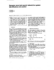
and can be used to control the secThus, the new inputs ondary flux amplitude and mover position, respectively. However, the secondary flux of the LIM is required to decouple the secondary flux dynamics from the motion dynamics completely. In this paper, an adaptive flux observer proposed by Lin et al. [27] is adopted to estimate the secondary flux. The detailed derivation of the adaptive flux observer is similar to [27] and is omitted here. A block diagram of the nonlinear decoupled LIM servo drive system combined with an adaptive flux observer is shown in Fig. 1, which consists of a ramp-comparison current-controlled pulsewidth modulated (PWM) voltage source inverter (VSI), a feedback linearization controller, two coordinate translators, a speed-control loop, and a position-control loop. The LIM used in this drive system is a three-phase Y-connected two-pole 3-kW 60-Hz 180-V/14.2-A type. The detailed parameters of the LIM are

(9) A From (9), the feedback linearization controller can be derived as follows: (10)

m

H H

where

is the flux current command.

H (13)


105

Fig. 2. Simplified position control system.

Fig. 3. Hybrid control system.

By using the nonlinear decoupled technique, the LIM servo drive shown in Fig. 1 can be reasonably represented by the control system block diagram shown in Fig. 2, in which (14) (15) is the thrust current command, and is the Laplace where operator. The curve-fitting technique based on step response is applied to find the drive model off line at the nominal case ). The results are (on a scale of 1.5915 (m/s)/V) ( N/WbA kg kg/s

Ns/V

where is a RFNN controller, and is a compensated is the main tracking concontroller. The RFNN control troller that is used to mimic a perfect control law, and the comis designed to compensate the difference pensated control between the perfect control law and the RFNN controller. The dynamic equation of the LIM servo drive system can be formulated by rewriting (12) as follows: (18) , where is the mover position of the LIM; , and . Define the tracking error vector as follows: (19)

N/V

(16)

The “ ” symbol represents the system parameters in the nominal condition. III. HYBRID CONTROL SYSTEM In order to control the mover position of the LIM effectively, a hybrid control system is proposed in this section. The configuration of the proposed hybrid control system, which combines a RFNN controller and a compensated controller, is shown in Fig. 3. The control law is assumed to take the following form [9]: (17)

and represent the desired mover position and where speed; is the tracking error of mover position. If the paramare well known, the eters of the LIM servo drive system and perfect control law which is designed in the sense of feedback linearization can be defined as follows [9]: (20) , in which and are positive conwhere stants. Substituting (20) into (18), it can be obtained (21) . Therefore, the perfect which implies that control law is an optimal-feedback linearization control law. However, the parameter variations of the system are difficult to

106

Fig. 4.


Structure of four-layer RFNN.

measure, and the exact value of the external force disturbance is also difficult to know in advance for practical applications. Therefore, a RFNN is proposed to mimic the perfect control law, and a compensated controller is proposed to compensate and the RFNN controller instead of the difference between increasing the rules of the RFNN.

Layer 2—Membership Layer: In this layer, each node performs a membership function. The Gaussian function is adopted as the membership function. For the th node

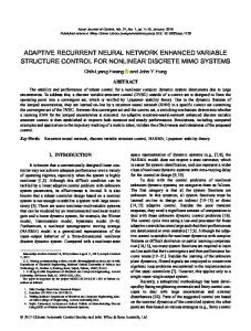
A. RFNN (23) A four-layer RFNN as shown in Fig. 4, which comprises the input (the layer), membership (the layer), rule (the layer), and output layer (the layer), is adopted to implement the RFNN controller in this paper. The signal propagation and the basic function in each layer of the RFNN are introduced as follows: Layer 1—Input Layer: For every node in this layer, the net input and the net output are represented as

and are, respectively, the mean and the standard where deviation of the Gaussian function in the th term of the th to the node of layer 2, and is the input linguistic variable total number of the linguistic variables with respect to the input nodes. Layer 3—Rule Layer: Each node in this layer is denoted by , which multiplies the input signals and outputs the result of product. For the th rule node

(22) where tions.

;

;

denotes the number of itera(24)


107

where th input to the node of layer 3; weights between the membership layer and the rule layer are assumed to be unity; recurrent weights for the units in the rule layer; number of rules with complete rule connection if each input node has the same linguistic variables. Layer 4—Output Layer: The single node in this layer is labeled with , which computes the overall output as the summation of all input signals

(25) is the output action strength where the connecting weight represents the of the th output associated with the th rule; th input to the node of layer 4, and . Moreover, can be rewritten as follows [11]:

will be proved in Section III-D. From (28), the error equation (27) can be rewritten as follows:

(29) Theorem 1: Consider the LIM servo drive system represented by (18), if the hybrid control law is designed as (17), in which the adaptation law of the RFNN is designed as (30) and the compensated controller is designed as (31), then asymptotical stability is guaranteed. (30) (31) where sgn is a sign function. Proof: A Lyapunov function is defined as

(26) (32) , in which is iniwhere tialized to be zero and adjusted during on-line operation; , in which is determined by the selected . membership function and Remark 1: The architecture of the RFNN used in this paper is designed to possess the advantage of simple structure with dynamic characteristics. The FNN proposed in [9], which has the merit of simple structure, is adopted to form the feedforward part of the RFNN. Moreover, the meaning of the recurrent is to consider the past firing strength of its corresponding rule in the rule layer owing to the feedback terms contain the firing history of the rules. Thus, the recurrent network has dynamic characteristics. In addition, the dynamic reasoning can be represented in the form: “If is and is and is , then is .”

where is a positive constant, and is a symmetric positive definite matrix which satisfies the following Lyapunov equation [28], [29]: (33) is selected by the designer. Take the derivative of the and Lyapunov function and use (29) and (33), then

B. Compensated Controller From (17), (18), and (20), an error equation is then obtained as follows: (27)

(34) Substitute (30) into (34) then

where (35) Use (31), thus is a stable matrix and . To develop the compensated controller, first, a minimum approximation error is defined as follows: (28) is an optimal weight vector achieves the minimum where approximation error, and the absolute value of is assumed to be ). The existence less than a small positive constant, (i.e., , i.e., the convergence of the RFNN, of finite value of

(36) , Since ), which implies

is negative semidefinite (i.e., and are bounded. Let function , and integrate function with

respect to time (37)

108


Because is bounded, and bounded, then

is nonincreasing and

The adaptation law of tion:

can be obtained by the following equa-

(38) Differentiate

(43)

with respect to time, then (39)

Since all the variables on the right-hand side (RHS) of (29) are is uniformly bounded, it implies is also bounded. Then continuous [28]. By using Barbalat’s lemma [28], [29], it can be . Therefore, as . shown that As a result, the hybrid control system is asymptotically stable. Moreover, the tracking error of the system will converge to . zero according to Remark 2: The minimum approximation error can be arbitrarily small by using more rules to construct the RFNN. However, the structure of the RFNN will become more complex with heavy computation load. To deal with the abovementioned problem, the proposed compensated controller can compensate the minimum approximation error and ensure the stability of the control system without increasing the number of rule. C. On-Line Parameter Training Selection of parameters for the membership functions and recurrent weights has a significant effect on the network performance. If inappropriate values are given for the membership functions and recurrent weights, the network will converge at a low speed. In order to train the RFNN effectively, an on-line parameter training methodology, which is derived using the Lyapunov stability theorem and the gradient descent method, is proposed. Not only the connecting weights between rule layer and output layer are adjusted on line but also the recurrent weights and the membership functions. This training scheme will increase the learning capability of the RFNN. The adaptation law shown in (30) can be rewritten as follows [9]: (40) is the learning-rate parameter of the weights in where the output layer and is some positive constant to be determined. According to the gradient descent method, the adaptation law of the weights in the output layer can be represented as follows:

In the membership layer, the error term is computed as follows:

(44) and also can be obtained by the The adaptation laws of gradient decent search algorithm, i.e., (45) (46) Remark 3: The derivations of the adaptation laws (43), (45), and (46) can help to overcome the inappropriate selection of the membership functions and the recurrent weights. It will not affect the stability property. D. Convergence Analyses of RFNN According to the assumption of the bound of the minimum approximation error, the stability proof of the hybrid control system can be guaranteed; however, the convergence condition of the RFNN must be satisfied. If the parameters of the RFNN are bounded, the convergence property of the RFNN can be guaranteed. From (26), the output of the RFNN is bounded if the weights between the output layer and the rule layer are bounded. for as Define the constrain set (47) is a two-norm of vector. According to the projection where algorithm [11], the adaptation law (30) can be modified as follows: if

if

(41) . The approximated error term needs Thus, to be calculated and propagated by the following equation:

or

and

and

(48) be defined in (47). If Theorem 2: Let the constraint set , the adaptation law the initial values of the weights for all . (48) guarantees that Proof: Define a Lyapunov function (49) Take the derivative of the Lyapunov function with respect to time

(42)

(50)


109

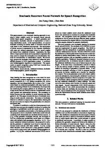
Fig. 5. DSP-based computer control system.

When the conditions ( ) hold, can be guaranteed that and the conditions

) or (

and . Thus, it . On the other hand, when hold,

(45), (46), and (48), and the compensated controller is designed as (31), then asymptotically stability is guaranteed. Proof: When the conditions or ( and ) hold, the stability analysis is the and same as Theorem 1. On the other hand, when , the derivative of the Lyapunov function shown in (34) can be rewritten as follows:

Thus, it also can be guaranteed that . Since the initial ), is value of is initialized to be zero (i.e., for all . bounded by the constraint set Remark 4: Since the convergence property of the RFNN can be guaranteed, it is reasonable that the minimum approximation error is assumed to be bounded. The bound of the approximation error is chosen to achieve the best transient control performance in both the simulation and experimentation considering the possible variation of operating conditions. E. Stability Analyses Using Projection Algorithm The modification of the adaptation law shown in (48) can guarantee that the weights between the output layer and the rule layer are bounded. Thus, the convergence property of the RFNN can be guaranteed. Moreover, the asymptotical stability of the proposed hybrid control system using the projection algorithm can be shown by the following theorem. Theorem 3: Consider the LIM servo drive system represented by (18), if the hybrid control law is designed as (17), in which the adaptation laws of the RFNN are designed as (43),

(51)

Use the property , which is according to

, and the

110

Fig. 6.


Sliding mode control system.

Fig. 7. Simulated results of sliding mode control system. (a) Mover position at Case 1. (b) Control effort at Case 1. (c) Mover position at Case 2.

By use of Barbalat’s lemma [28], [29] as shown in Theorem 1, as . Thus, the stability property also can be guaranteed. The effectiveness of the hybrid control system using RFNN based on the proposed on-line parameter training methodology is demonstrated by the following simulated and experimental results.

compensated controller shown in (31), then

IV. SIMULATION AND EXPERIMENTATION (52)

A block diagram of the DSP-based computer control system for a LIM servo drive using the current-controlled technique


Fig. 7. (Continued.)

111

Simulated results of sliding mode control system. (d) Control effort at Case 2. (e) Mover position at Case 3. (f) Control effort at Case 3.

is shown in Fig. 5. The current-controlled PWM VSI is implemented by an IPM switching component (PM50RSA060) manufactured by Mitsubishi Co. with a switching frequency of 15 kHz. A servo control card is installed in the control computer, which includes multichannels of D/A and encoder interface circuits. Digital filter and frequency multiplied by four circuits are built into the encoder interface circuit to increase the precision of position feedback. The resulting precision is one pulse to 50 m. The feedback linearization controller and the hybrid control system are realized in a Pentium CPU, moreover, the adaptive flux observer is realized in a TMS320C31 DSP. Three-phase voltages and currents are sampled by the A/D converters connected to the DSP to provide input signals for the observation system. The control intervals of the feedback linearization controller and the observation system are set at 0.2 ms, and the control interval of the position control loop is set at 1 ms. The control objective is to control the mover to move 0.1 m to 0.1 m periodically. The gains of the hybrid control system are given in the following equation: (53)

All the gains in the hybrid control system are chosen to achieve the best transient control performance in both the simulation and experimentation considering the requirement of stability, limitation of control effort, and possible operating conditions. To show the effectiveness of the RFNN control with small rule set, the RFNN has two, six, nine, and one neurons at the input, membership, rule, and output layers, respectively. It can be regarded that the associated fuzzy sets with Gaussian function for each input signal are divided into N (negative), Z (zero), and P (positive), and the number of rules with complete rule connection is nine ( ). On the other hand, if the RFNN is designed with small numbers of neurons at membership and rule layers, the convergence of tracking error is slow. Moreover, if the RFNN is designed with large numbers of neurons at membership and rule layers, the improvement of control performance is limited, and the computation burden for the CPU is significantly increased. In addition, some heuristics can be used to roughly initialize the parameters of the RFNN for practical applications, e.g., the mean and standard deviation of the Gaussian functions can be determined according to the maximum variand . The effect due to the inaccurate selecation of tion of the initialized parameters can be retrieved by the on-line

112


Fig. 8. Simulated results of hybrid control system. (a) Mover position at Case 1. (b) Control effort at Case 1. (c) Mover position at Case 2.

training methodology. Therefore, for simplicity, the means of , 0, 1 for the N, Z, P neuthe Gaussian functions are set at rons, and the standard deviations of the Gaussian functions are set at 1. A. Simulation To investigate the effectiveness of the sliding mode and hybrid control systems, three cases with parameter variations and external force disturbance are considered here. Case 1: (54) (55)

Case 2: Case 3:

at 3 s.

(56)

To show the advantages of the proposed hybrid control system, the sliding-mode control designed by Slotine and Li [28] is adopted here for comparison. The adopted sliding mode control law is (57)

where is the geometric mean of the bounded by known , in which and are the upper and constants ; is the selected sliding surlower bounds of the face, in which is a positive constant setting at 1 for simplicity; is the equivalent control; is the control gain to satisfy the sliding condition. The block diagram of the sliding mode control system is shown in Fig. 6. Selection of the control gain is relative to the magnitude of uncertainties to keep the trajectory on the sliding surface. However, the parameter variations of the system are difficult to measure, and the exact value of the external force disturbance is also difficult to know in advance for practical applications. To demonstrate the effect of the selection of the control gain in sliding-mode control, the control gain is set at 10 only considering the possible parameter variations in the simulation. The simulated results of the sliding-mode control system due to periodic sinusoidal command at Case 1, Case 2, and Case 3 are shown in Fig. 7, in which the position responses of the mover at Case 1, Case 2, and Case 3 are shown in Fig. 7(a), (c), and (e); the associated control efforts are shown in Fig. 7(b), (d), and (f). Though favorable tracking responses can be obtained by the sliding mode controller as shown in Fig. 7(a) and (c), the chattering control efforts are caused by the switching operation. Moreover, since the


113

Fig. 8. (Cont’d) Simulated results of hybrid control system. (d) Control effort at Case 2. (e) Mover position at Case 3. (f) Control effort at Case 3.

external force disturbance is not considered in the selection of control gain, unstable tracking performance is resulted as shown in Fig. 7(e) due to the inappropriate selection of the control gain. Though large control gain may solve the problem of unstable or slow tracking responses, it will result impractical large control efforts. Therefore, the control gain is difficult to determine due to the unknown uncertainties in practical applications, and is ordinarily chosen as a compromise between the stability and control performance. On the other hand, the simulated results of the hybrid control system due to periodic sinusoidal command at Case 1, Case 2, and Case 3 are shown in Fig. 8, in which the position responses of the mover at Case 1, Case 2, and Case 3 are shown in Fig. 8(a), (c), and (e); the associated control efforts are shown in Fig. 8(b), (d), and (f). Since all the parameters of the RFNN are roughly initialized, accurate tracking control performance of the LIM servo drive can be obtained after one cycle of on-line training of the RFNN for periodic sinusoidal command. However, the chattering phenomena do not exist in the control efforts of the hybrid control system as shown in Fig. 8(b), (d), and (f). In addition, the robust control performance of the hybrid control system, both in the conditions of parameter variations and external force disturbance, is obvious as shown in Fig. 8(c) and (e). From the simulated results, the proposed hybrid control

system is more suitable to control the mover position of the LIM servo drive system. B. Experimentation Some experimental results are provided to demonstrate the control performance of the sliding-mode and hybrid control systems. Two test conditions are provided in the experimentation, which are the nominal case and the parameter variation case. The parameter variation case is the addition of one iron disk with 8.34 kg weight to the mass of the mover, i.e., the total mass is four times the nominal mass. The experimental results ) due to periodic siof the sliding mode control system ( nusoidal command at the nominal case and the parameter variation case are shown in Fig. 9, in which the position responses of the mover at the nominal case and the parameter variation case are shown in Fig. 9(a) and (c); the associated control efforts are shown in Fig. 9(b) and (d). Though favorable tracking responses can be obtained by the sliding-mode controller, the chattering phenomena existed in the control efforts result in inaccurate tracking responses. Moreover, the chattering control efforts will wear the bearing mechanism and might excite unstable system dynamics. On the other hand, the experimental results

114

Fig. 9. Experimental results of sliding mode control system. (a) Mover position at nominal case. (b) Control effort at nominal case. (c) Mover position at parameter variation case. (d) Control effort at parameter variation case.

of the hybrid control system due to periodic sinusoidal command at the nominal case and the parameter variation case are shown in Fig. 10, in which the position responses of the mover at the nominal case and the parameter variation case are shown in Fig. 10(a) and (c); the associated control efforts are shown in Fig. 10(b) and (d). Since all the parameters of the RFNN are roughly initialized, accurate tracking control performance of the LIM servo drive can be obtained after one cycle of on-line training of the RFNN for periodic sinusoidal command. However, the chattering phenomena are not existed in the control efforts of the hybrid control system as shown in Fig. 10(b) and (d). In addition, the robust control performance of the hybrid control system under the occurrence of the parameter variations is ob-


Fig. 10. Experimental results of hybrid control system. (a) Mover position at nominal case. (b) Control effort at nominal case. (c) Mover position at parameter variation case. (d) Control effort at parameter variation case.

vious as shown in Fig. 10(d). From the experimental results, the control performance of the proposed hybrid control system is better than the sliding mode control system for the tracking of periodic commands.

V. CONCLUSION This paper has successfully demonstrated the applications of a hybrid control system to the periodic motion control of a LIM servo drive. First, the feedback linearization theory was used to decouple the thrust force and the flux amplitude of the LIM.


Then, a hybrid control system was proposed to control the periodic motion of the mover of the LIM. In the hybrid control system, the RFNN controller is the main tracking controller, which is used to mimic a perfect control law, and the compensated controller is designed to guarantee the asymptotical stability of the hybrid control system. Moreover, an on-line parameter training methodology, which is derived using the Lyapunov stability theorem and the gradient descent method, was proposed to increase the learning capability of the RFNN. Not only the connecting weights between rule layer and output layer are adjusted on line but also the recurrent weights and the membership functions. The effectiveness of the proposed hybrid control scheme has been confirmed by some simulated and experimental results. Compared with the sliding-mode controller, the merits of the hybrid control system for the tracking of periodic reference inputs are: 1) small control effort; 2) alleviation of chattering phenomenon; and 3) without using prior knowledge of the controlled plant in the design of controller. REFERENCES [1] K. S. Narendra and K. Parthasarathy, “Identification and control of dynamical systems using neural networks,” IEEE Trans. Neural Networks, vol. 1, pp. 4–27, 1990. [2] Y. M. Park, M. S. Choi, and K. Y. Lee, “An optimal tracking neuro-controller for nonlinear dynamic systems,” IEEE Trans. Neural Networks, vol. 7, pp. 1099–1110, 1996. [3] S. C. Sivakumar, W. Robertson, and W. J. Phillips, “On-line stabilization of block-diagonal recurrent neural networks,” IEEE Trans. Neural Networks, vol. 10, pp. 167–175, 1999. [4] C. C. Ku and K. Y. Lee, “Diagonal recurrent neural networks for dynamic systems control,” IEEE Trans. Neural Networks, vol. 6, pp. 144–156, 1995. [5] M. A. Brdys and G. J. Kulawski, “Dynamic neural controllers for induction motor,” IEEE Trans. Neural Networks, vol. 10, pp. 340–355, 1999. [6] T. W. S. Chow and Y. Fang, “A recurrent neural-network-based real-time learning control strategy applying to nonlinear systems with unknown dynamics,” IEEE Trans. Indust. Electron., vol. 45, pp. 151–161, 1998. [7] Y. Fang, T. W. S. Chow, and X. D. Li, “Use of a recurrent neural network in discrete sliding-mode control,” IEE Proc. Contr. Theory Applicat., vol. 146, no. 1, pp. 84–90, 1999. [8] F. J. Lin, R. J. Wai, and H. P. Chen, “A PM synchronous servo motor drive with an on-line trained fuzzy neural network controller,” IEEE Trans. Energy Conversion, vol. 13, pp. 319–325, 1998. [9] F. J. Lin, W. J. Hwang, and R. J. Wai, “A supervisory fuzzy neural network control system for tracking periodic inputs,” IEEE Trans. Fuzzy Syst., vol. 7, pp. 41–52, Feb. 1999. [10] Y. C. Chen and C. C. Teng, “A model reference control structure using a fuzzy neural network,” Fuzzy Sets Syst., vol. 73, pp. 291–312, 1995. [11] L. X. Wang, A Course in Fuzzy Systems and Control. Englewood Cliffs, NJ: Prentice-Hall, 1997. [12] J. Zhang and A. J. Morris, “Recurrent neuro-fuzzy networks for nonlinear process modeling,” IEEE Trans. Neural Networks, vol. 10, pp. 313–326, 1999. [13] C. F. Juang and C. T. Lin, “A recurrent self-organizing neural fuzzy inference network,” IEEE Trans. Neural Networks, vol. 10, pp. 828–845, 1999. [14] I. Takahashi and Y. Ide, “Decoupling control of thrust and attractive force of a LIM using a space vector control inverter,” IEEE Trans. Indust. Applicat., vol. 29, pp. 161–167, 1993. [15] I. Boldea and S. A. Nasar, Linear Electric Actuators and Generators. Cambridge, U.K.: Cambridge University Press, 1997. [16] Z. Zhang, T. R. Eastham, and G. E. Dawson, “Peak thrust operation of linear induction machines from parameter identification,” in IEEE IAS Conf. Rec., 1995, pp. 375–379.

115

[17] G. Bucci, S. Meo, A. Ometto, and M. Scarano, “The control of LIM by a generalization of standard vector techniques,” in IEEE IAS Conf. Rec., 1994, pp. 623–626. [18] Z. Zhang, G. E. Dawson, and T. R. Eastham, “Microcontroller based on-line identification of variable parameters in induction motors,” Electric Machine Power Syst., vol. 23, pp. 353–360, 1995. [19] D. W. Novotny and T. A. Lipo, Vector Control and Dynamics of AC Drives. Oxford, U.K.: Clarendon, 1996. [20] C. C. Chan and H. Wang, “An effective method for rotor resistance identification for high-performance induction motor vector control,” IEEE Trans. Indust. Electron., vol. 37, pp. 477–482, 1990. [21] F. J. Lin, H. M. Su, and H. P. Chen, “Induction motor servo drive with adaptive rotor time-constant estimation,” IEEE Trans. Aerosp. Electron. Syst., vol. 34, pp. 224–234, 1998. [22] G. S. Kim, I. J. Ha, and M. S. Ko, “Control of induction motors for both high dynamic performance and high power efficiency,” IEEE Trans. Indust. Electron., vol. 39, pp. 323–333, 1992. [23] R. Marino, S. Peresada, and P. Valigi, “Adaptive input–output linearizing control of induction motors,” IEEE Trans. Automat. Contr., vol. 38, pp. 208–221, 1993. [24] M. Bodson, J. Chiasson, and R. Novotnak, “High-performance induction motor control via input–output linearization,” IEEE Contr. Syst. Mag., vol. 14, pp. 25–33, 1994. [25] W. J. Wang and C. C. Wang, “Composite adaptive position controller for induction motor using feedback linearization,” IEE Proc. Contr. Theory Applicat., vol. 145, pp. 25–32, 1998. [26] H. J. Shieh and K. K. Shyu, “Nonlinear sliding-mode torque control with adaptive backstepping approach for induction motor drive,” IEEE Trans. Indust. Electron., vol. 46, pp. 380–389, 1999. [27] F. J. Lin, R. J. Wai, and P. C. Lin, “Robust speed sensorless induction motor drive,” IEEE Trans. Aerosp. Electron. Syst., vol. 35, pp. 566–578, 1999. [28] J. J. E. Slotine and W. Li, Applied Nonlinear Control. Englewood Cliffs, NJ: Prentice-Hall, 1991. [29] K. J. Astrom and B. Wittenmark, Adaptive Control. New York: Addison-Wesley, 1995.

Faa-Jeng Lin (M’93–SM’99) received the B.S. and M.S. degrees from National Cheng Kung University, Tainan, Taiwan, R.O.C., and the Ph.D. degree from National Tsing Hua University, Hsin Chu, Taiwan, R.O.C., in 1983, 1985, and 1993, respectively, all in electrical engineering. During 1985–1989, he was with the Chung-Shan Institute of Science and Technology as a Group Leader of Automatic Test Equipment and Microcomputer System Design Division. He is currently Professor in the Department of Electrical Engineering, Chung Yuan Christian University, Chung Li, Taiwan, R.O.C. His research interests include motor servo drives, computer-based control systems, control theory applications, power electronics, and mechatronics.

Rong-Jong Wai (M’00) was born in Tainan, Taiwan, in 1974. He received the B.S. degree in electrical engineering and the Ph.D. degree in electronic engineering from the Chung Yuan Christian University, Chung-Li, Taiwan, in 1996 and 1999, respectively. Since 1999, he has been with the Department of Electrical Engineering, Yuan Ze University, Chung-Li, Taiwan, where he is currently an Assistant Professor. His research interests include motor servo drives, mechatronics, nonlinear control, and intelligent control system including neural networks and fuzzy logic. He is the chapter-author of Intelligent Adaptive Control: Industrial Applications in the Applied Computational Intelligence Set (CRC Press LLC, 1998) and the co-author of Drive and Intelligent Control of Ultrasonic Motor (Taiwan: Tsang-Hai, 1999). He is a member of the IEEE Industrial Electronics Society.