Hybrid In-Database Inference for Declarative ... - Semantic Scholar

Hybrid In-Database Inference for Declarative Information Extraction Daisy Zhe Wang

Michael J. Franklin

University of California, Berkeley

University of California, Berkeley

Minos Garofalakis

Joseph M. Hellerstein

Michael L. Wick

Technical University of Crete

University of California, Berkeley

University of Massachusetts, Amherst

ABSTRACT

1

In the database community, work on information extraction (IE) has centered on two themes: how to effectively manage IE tasks, and how to manage the uncertainties that arise in the IE process in a scalable manner. Recent work has proposed a probabilistic database (PDB) based declarative IE system that supports a leading statistical IE model, and an associated inference algorithm to answer top-k-style queries over the probabilistic IE outcome. Still, the broader problem of effectively supporting general probabilistic inference inside a PDB-based declarative IE system remains open. In this paper, we explore the in-database implementations of a wide variety of inference algorithms suited to IE, including two Markov chain Monte Carlo algorithms, the Viterbi and the sum-product algorithms. We describe the rules for choosing appropriate inference algorithms based on the model, the query and the text, considering the trade-off between accuracy and runtime. Based on these rules, we describe a hybrid approach to optimize the execution of a single probabilistic IE query to employ different inference algorithms appropriate for different records. We show that our techniques can achieve up to 10-fold speedups compared to the non-hybrid solutions proposed in the literature.

For most organizations, textual data is an important natural resource to fuel data analysis. Information extraction (IE) techniques parse raw text and extract structured objects that can be integrated into databases for querying. In the past few years, declarative information extraction systems [1, 2, 3, 4] have been proposed to effectively manage IE tasks. The results of IE extraction are inherently uncertain, and queries over those results should take that uncertainty into account in a principled manner. Research in probabilistic databases (PDBs) has been exploring scalable tools to reason about these uncertainties in the context of structured query languages and query processing [5, 6, 7, 8, 9, 10, 11, 12]. Our recent work [4, 13] has proposed a PDB system that natively supports a leading statistical IE model (conditional random fields (CRFs)), and an associated inference algorithm (Viterbi). It shows that the in-database implementation of the inference algorithms enables: (1) probabilistic relational queries that returns top-k results over the probabilistic IE outcome; (2) a tight integration between the relational and inference operators, which leads to significant speed-up by performing query-driven inference. While this work is an important step towards building a probabilistic declarative IE system, the approach is limited by the capabilities of the Viterbi algorithm, which can only handle top-k-style queries over a limited class of CRF models: linear chain models, which do a poor job capturing features like repeated terms. Different inference algorithms are needed to deal with non-linear CRF models, such as skip-chain CRF models, complex IE queries that induce cyclic models over the linear-chain CRFs, and marginal inference queries that produce richer probabilistic outputs than top-k. The broader problem of effectively supporting general probabilistic inference inside a PDB-based declarative IE system remains open. In this paper, we first explore the in-database implementation of a number of inference algorithms suited to a broad variety of models and outputs: two variations of the general sampling-based Markov chain Monte Carlo (MCMC) inference algorithm—Gibbs Sampling and MCMC Metropolis-Hastings (MCMC-MH)—in addition to the Viterbi and the sum-product algorithms. We compare the applicability of these four inference algorithms and study the data and the model parameters that affect the accuracy and runtime of those algorithms. Based on those parameters, we develop a set of rules for choosing an inference algorithm based on the characteristics of the model and the data. More importantly, we study the integration of relational query processing and statistical inference algorithms, and demonstrate that, for SQL queries over probabilistic extraction results, the proper choice of IE inference algorithm is not only model-dependent, but also query- and text-dependent. Such dependencies arise when re-

Categories and Subject Descriptors H.2.4 [Database Management]: Systems—Textual databases, Query Processing; G.3 [Mathematics of Computing]: Probability and statistics—Probabilistic algorithms (including Monte Carlo)

General Terms Algorithms, Performance, Management, Design

Keywords Probabilistic Database, Probabilistic Graphical Models, Information Extraction, Conditional Random Fields, Viterbi, Markov chain Monte Carlo Algorithms, Query Optimization

Permission to make digital or hard copies of all or part of this work for personal or classroom use is granted without fee provided that copies are not made or distributed for profit or commercial advantage and that copies bear this notice and the full citation on the first page. To copy otherwise, to republish, to post on servers or to redistribute to lists, requires prior specific permission and/or a fee. SIGMOD’11, June 12–16, 2011, Athens, Greece. Copyright 2011 ACM 978-1-4503-0661-4/11/06 ...$10.00.

Introduction

lational queries are applied to the CRF model, inducing additional variables, edges and cycles; and when the model is instantiated over different text, resulting in model instances with drastically different characteristics. To achieve good accuracy and runtime performance, it is imperative for a PDB system to use a hybrid approach to IE even within a single query, employing different algorithms for different records. In the context of our CRF-based PDB system, we describe query processing steps and an algorithm to generate query plans that apply hybrid inference for probabilistic IE queries. Finally, we describe example queries and experiment results showing that such hybrid inference techniques can improve the runtime of the query processing by taking advantage of the appropriate inference methods for different combinations of query, text, and CRF model parameters. Our key contributions can be summarized as follows: • We show the efficient implementation of two MCMC inference algorithms, in addition to the Viterbi and the sumproduct algorithms, and we identify a set of parameters and rules for choosing different inference algorithms over models and datasets with different characteristics; • We describe query processing steps and an algorithm to generate query plans that employ hybrid inference over different text within the same query, where the selection of the inference algorithm is based on all three factors of data, model, and query; • Last, we evaluate our approaches and algorithms using three real-life datasets: DBLP, NYTimes, and Twitter. The results show that our hybrid inference techniques can achieve up to 10-fold speedups compared to the non-hybrid solutions proposed in the literature. Based on our experience in implementing different inference algorithms, we also present four design guidelines for implementing statistical methods in the database in the Appendix.

2

Related Work

In the past few years, declarative information extraction systems [1, 2, 3, 4, 13] have been proposed to effectively manage information extraction (IE) tasks. The earlier efforts in declarative IE [1, 2, 3] lack a unified framework supporting both a declarative interface as well as the state-of-the-art probabilistic IE models. Ways to handle uncertainties in IE have been considered in [14, 15]. A probabilistic declarative IE system has been proposed in [4, 13], but it only supports the Viterbi algorithm, which is unable to handle complex models that arise naturally from advanced features and relational operators. In the past decade, there has been a groundswell of work on Probabilistic Database Systems (PDBS) [5, 6, 7, 8, 9, 10, 11, 12]. As shown in previous work [8, 10, 12], Graphical Modeling techniques can provide robust statistical models that capture complex correlation patterns among variables, while, at the same time, addressing some computational efficiency and scalability issues as well. In addition, [8] showed that other approaches to represent and handle uncertainty in database [5, 6], can be unified under the framework of Graphical Models, which express uncertainties and dependencies through the use of random variables and joint probability distribution. However, there is no work addressing the problem of effectively supporting and optimizing different probabilistic inference algorithms in a single PDB, especially in the IE setting.

3

Background

This section covers our definition of a probabilistic database, the conditional random fields (CRF) model and the different types of inference algorithms over CRF models in the context of information extraction. We also introduce a template for the types of IE queries studied in this paper. 3.1

Probabilistic Database

As we described in [10], a probabilistic database DBp consists of two key components: (1) a collection of incomplete relations R with missing or uncertain data, and (2) a probability distribution F on all possible database instances, which we call possible worlds, and denote by pwd(DBp ). An incomplete relation R ∈R is defined over a schema Ad ∪ Ap comprising a (non-empty) subset Ad of deterministic attributes (that includes all candidate and foreign key attributes in R), and a subset Ap of probabilistic attributes. Deterministic attributes have no uncertainty associated with any of their values. A probabilistic attribute Ap may contains missing or uncertain values. The probabilistic distribution F of these missing or uncertain values is represented by a probabilistic graphical model, such as Baysian Networks or Markov Random Fields. Each possible database instance is a possible completion of the missing and uncertain data in R. 3.2

Conditional Random Fields

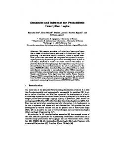
The linear-chain CRF [16, 17], similar to the hidden markov model, is a leading probabilistic model for solving IE tasks. In the context of IE, a CRF model encodes the probability distribution over a set of label random variables (RVs) Y, given the value of a set of token RVs X. We denote an assignment to X by x and to Y by y. In a linear-chain CRF model, label yi is correlated only with label yi−1 and token xi . Such correlations are represented by the feature functions {fk (yi , yi−1 , xi )}K k=1 . E XAMPLE 1. Figure 1(a) shows an example CRF model over an address string x ’2181 Shattuck North Berkeley CA USA’. Observed (known) variables are shaded nodes in the graph. Hidden (unknown) variables are unshaded. Edges in the graph denote statistical correlations. The possible labels are Y = {apt.num, streetnum, streetname, city, state, country}. Two possible feature functions of this CRF are: f1 (yi , yi−1 , xi ) f2 (yi , yi−1 , xi )

= =

[xi appears in a city list] · [yi = city] [xi is an integer] · [yi = apt.num] ·[yi−1 = streetname]

A segmentation y = {y1 , ..., yT } is one possible way to tag each token in x of length T with one of the labels in Y . Figure 1(d) shows two possible segmentations of x and their probabilities. D EFINITION 3.1. Let {fk (yi , yi−1 , xi )}K k=1 be a set of realvalued feature functions, and Λ = {λk } ∈ RK be a vector of real-valued parameters, a CRF model defines the probability distribution of segmentations y given a specific token sequence x: p(y | x) =

T X K X 1 exp{ λk fk (yi , yi−1 , xi )}, Z(x) i=1 k=1

(1)

where Z(x) is a standard normalization function that guarantees the probability distribution sums to 1 over all possible extractions.  3.3

Relational Representation of Text and CRF

We implement IE algorithms over the CRF model within a database using the relational representations of text and the CRF-based distribution in the token table T OKEN T BL and the factor table MR respectively.

3.5

Y=labels (a) X=tokens 2181

Shattuck

id docID pos token

North

Berkeley

token

Label

CA

USA

prevLabel label

score

1

1

0

2181

2181 (DIGIT) null

street num

22

2

1

1

Shattuck

2181 (DIGIT) null

street name

5

3

1

2

North

(b) …

(c)

..

..

street

street name

10 25

4

1

3

Berkeley

Berkeley

5

1

4

CA

Berkeley

street

city

6

1

5

USA

..

..

..

x

2181

Shattuck

North

Berkeley CA

y1

street num

street name

city

city

state country

(0.6)

y2

street num

street name

street name

city

state country

(0.1)

Viterbi, a special case of the Max-Product algorithm [19, 20] can compute top-k inference for linear-chain CRF models. Viterbi is a dynamic programming algorithm that computes a two dimensional V matrix, where each cell V (i, y) stores a ranked list of partial label sequences (i.e., paths) up to position i ending with label y and ordered by score. Based on Equation (1), the recurrence to compute the top-1 segmentation is as follows:  0 0 (V (i − 1, y )  maxyP V (i, y) = + K λ f (y, y 0 , xi )), k k k=1  0,

USA (d)

Figure 1: (a) Example CRF model; (b) Example T OKEN T BL table; (c) Example MR table; (d) Two possible segmentations y1 , y2 . Token Table: The token table T OKEN T BL, as shown in Figure 1(b), is an incomplete relation R in DBp , which stores a set of documents or text-strings D as a relation in a database, in a manner akin to the inverted files commonly used in information retrieval. T OKEN T BL (id, docID, pos, token, labelp )

T OKEN T BL contains one probabilistic attribute—labelp , and the main goal of IE is to perform inference on labelp . As shown in the schema above, each tuple in T OKEN T BL records a unique occurrence of a token, which is identified by the text-string ID (docID) and the position (pos) the token is taken from. The id field is simply a row identifier for the token in T OKEN T BL. Factor Table: The probability distribution F over all possible “worlds” of T OKEN T BL can be computed from the MR. The MR is a materialization of the factor tables in the CRF model for all the tokens in the corpus D. The factor tables φ[yi , yi−1 | xi ], as shown in Figure 1(c), represent the correlation between xi , yi , and yi−1 , and are computed by the weighted sum of Pa set of feature functions in the CRF model: φ[yi , yi−1 | xi ] = K k=1 λk fk (yi , yi−1 , xi ). As in the following schema, each unique token string xi is associated with an array, which contains a set of scores ordered by {prevLabel, label}. MR (token, score ARRAY[])

3.4

Viterbi Algorithm

Inference Queries over a CRF Model

There are two types of inference queries over the CRF model [17]. • Top-k Inference: The top-k inference computes the label sequence y (i.e., extraction) with the top-k highest probabilities given a token sequence x from a text-string d. Constrained top-k inference [18] is a special case, where the topk extractions are computed, conditioned on a subset of the token labels, that are provided as evidence. • Marginal Inference: Marginal inference computes a marginal probability p(yt , yt+1 , ..., yt+k |x, s) over a single label or a sub-sequence of labels conditioned on the set of evidence s = {s1 , ..., sT }, where si is either NULL (i.e., no evidence) or the evidence label for yi . Many inference algorithms are known that can answer the above inference queries over the CRF models, varying in their effectiveness for different CRF characteristics (e.g., shape of the graph). In the next sections, three inference algorithms will be described: Viterbi, sum-product, Markov chain Monte Carlo (MCMC) methods.

if if

i>0 i = −1.

(2)

The top-1 extraction y ∗ can be backtracked from the maximum entry in V (T, yT ), where T is the length of the token sequence x. The complexity of the Viterbi algorithm is O(T · |Y |2 ), where |Y | is the number of possible labels. The constrained top-k inference can be computed by a variant of the Viterbi algorithm which restricts the chosen labels y to conform with the evidence s. 3.6

Sum-Product Algorithm

Sum-product (i.e., belief propagation) is a message passing algorithm for performing inference on graphical models, such as CRF [19]. The simplest form of the algorithm is for tree-shaped models, in which case the algorithm computes exact marginal distributions. The algorithm works by passing real-valued functions called messages along the edges between the nodes. These contain the “influence” that one variable exerts on another. A message from a variable node yv to its “parent” variable node yu in a tree-shaped model is computed by summing the product of the messages from all the “child” variables of yv in C(yv ) and the feature function f (yu , yv ) between yv and yu over variable yv : µyv →yu (yu ) =

X yv

Y

f (yu , yv )

∗ →y (yv ). µyu v

(3)

∗ ∈C(y ) yu v

Before starting, the algorithm first designates one node as the root; any non-root node which is connected to only one other node is called a leaf. In the first step, messages are passed inwards: starting at the leaves, each node passes a message along the edge towards the root node. This continues until the root has obtained messages from all of its adjoining nodes. The marginal of the root note can be computed at the end of the first step. The second step involves passing the messages back out: starting at the root, messages are passed in the reverse direction, until all leaves have received their messages. Like Viterbi, the complexity of the sum-product algorithm is also O(T · |Y |2 ). Variants of the sum-product algorithm for cyclic models require either an intractable junction-tree step, or a variational approximation such as loopy belief propagation (BP). In this paper, we do not study these variants further as they are either intractable (junction tree), or can fail to converge (loopy BP) on models with longdistance dependencies such as those we discussed in this paper. 3.7

MCMC Inference Algorithms

Markov chain Monte Carlo (MCMC) methods are a class of randomized algorithms for estimating intractable probability distributions over large state spaces by constructing a Markov chain sampling process that converges to the desired distribution. Relative to other sampling methods, the main benefits of MCMC methods are that they (1) replace a difficult sampling procedure from a highdimensional target distribution π(w) that we wish to sample with an easy sampling procedure from a low-dimensional local distribution q(·|w), and (2) sidestep the #P -hard computational problem of computing a normalization factor. We call q(·|w) a “pro-

G IBBS (N ) w0 ← I NIT(); w ← w0 ; // initialize for idx = 1, ..., N do i ← idx%n; // propose variable to sample next w0 ∼ π(wi | w−i ) // generate sample return next w0 // return a new sample w ← w0 ; // update current world endfor

SELECT

1 2 3 4 5 6 7

Figure 2: Pseudo-code for Gibbs sampling algorithm over a model with n variables. posal distribution”, which—conditioned on a previous state w— probabilistically produces a new world w0 with probability q(w0 |w). In essence, we use the proposal distribution to control a random walk among points in the target distribution. We review two MCMC methods we will adapt to our context in this paper: Gibbs sampling and Metropolis-Hastings (MCMC-MH). 3.7.1

Gibbs Sampling

Let w = (w1 , w2 , ..., wn ) be a set of n random variables, distributed according to π(w). The proposal distribution of a specific variable wi is its marginal distribution q(·|w) = π(wi |w−i ) conditioned on w−i , which are the current values of the rest of the variables. The Gibbs sampling algorithm (i.e., Gibbs sampler) first generates the initial world w0 , for example, randomly. Next, samples are drawn for each variable wi ∈ w in turn, from the distribution π(wi |w−i ). Figure 2 shows the pseudo-code for the Gibbs sampler that returns N samples. In Line 4, ∼ means a new sample w0 is drawn according to the proposal distribution π(wi |w−i ). 3.7.2

Metropolis-Hastings (MCMC-MH)

Like Gibbs, the MCMC-MH algorithm first generates an initial world w0 (e.g., randomly). Next, samples are drawn from the proposal distribution w0 ∼ q(wi |w), where a variable wi is randomly picked from all variables, and q(wi |w) is a uniform distribution over all possible values. Different proposal distribution q(wi |w) can be used, which results in different convergence rates. Lastly, each resulting sample is either accepted or rejected according to a Bernoulli distribution given by parameter α: α(w0 , w) = min(1,

π(w0 )q(w|w0 ) ) π(w)q(w0 |w)

(4)

The acceptance probability is determined by the product of two ratios: the model probability ratio π(w0 )/π(w), which captures the relative likelihood of the two worlds; and the proposal distribution ratio q(w|w0 )/q(w0 |w), which eliminates the bias introduced by the proposal distribution. 3.8

Query Template

Over the CRF-based IE from text, the queries we consider are probabilistic queries, which inference over the probabilistic attribute labelp in the T OKEN T BL table. Each T OKEN T BL is associated with a specific CRF model stored in the MR table. Such CRFbased IE is captured by a sub-query with logic that produces the IE results from the base probabilistic T OKEN T BL tables. The subquery consists of a relational part Qre over the probabilistic token tables T OKEN T BL and the underlying CRF models, followed by an inference operator Qinf . A canonical “query template” captures the logic for the “SQL+IE” sub-query in Figure 3. It supports SPJ queries, aggregate conditions and two types of inference operators, Top-k and Marginal, over the probabilistic T OKEN T BL tables. The relational part of a “SQL+IE” query Qre first specifies, in the FROM clause, the T OKEN T BL table(s) over which the query and extraction is performed.

Top-k(T1.docID,[T1.pos|exist]) | [Marginal(T1.docID,[T1.pos|exist])] | [Top-k(T1.docID, T2.docID,[T1.pos|T2.pos|exist])] | [Marginal(T1.docID,T2.docID,[T1.pos|T2.pos|exist])] FROM TokenTbl1 T1[, TokenTbl2 T2] WHERE T1.label = ’bar1’ [and T1.token = ’foo1’] [and T1.docID = X] [and T1.pos = Y] [and T1.label = T2.label] [and T1.token = T2.token] [and T1.docID = T2.docID] GROUP BY T1.docID[, T2.docID] HAVING [aggregate condition]

Figure 3: The “SQL+IE” query template. The WHERE clause lists a number of possible selection as well as join conditions over the T OKEN T BL tables. These conditions when involve labelp are probabilistic conditions, and deterministic otherwise. For example, a probabilistic condition label=’person’ specifies the entity types we are looking for is ’person’, while a deterministic condition token=’Bill’ specifies the name of the entity we are looking for is ’Bill’. We can also specify a join condition T1.token=T2.token and T1.label=T2.label that two documents need to contain the same entity name with the same entity type. In the GROUP BY and the HAVING clause, we can specify conditions on an entire text “document”. An example of such aggregate condition over a bibliography document can be that all title tokens are in front of all the author tokens. Following the Possible World Semantics [5], the execution of these relational operators involve modification to the original graphical models as will be shown in Section 4.1. The inference part Qinf , of a “SQL+IE” query, takes the docID, the pos, and the CRF model resulting from Qre as input. The inference operation is specified in the SELECT clause, which can be either a Top-k or a Marginal inference. The inference can be computed over different random variables in the CRF model: (1) a sequence of tokens (e.g., a document) specified by docID; or (2) a token at a specific location specified by docID and pos; or (3) the “existence” (exist) of the result tuple. The “existence” of the result tuple becomes probabilistic with a selection or join over a probabilistic attribute, where exist variables are added to the model [10]. For example, the inference Marginal(T1.docID,T1.pos), for each position (T1.docID,T1.pos) computed from Qre , returns the distribution of the label variable at that position. The inference Marginal(T1.docID,exist) computes the marginal distribution of exist variable for each result tuple. We can also specify an inference following a join query. For example, the inference Top-k(T1.docID,T2.docID), for each document pair (T1.docID,T2.docID), returns the top-k highest probability joint extractions that satisfy the join constraint.

4

In-Database MCMC Inference

In this section, we first describe IE models that are cyclic (e.g., the skip-chain CRF model) and review the way that simple relational queries can often induce cyclic models—even over text that is itself modeled by simple linear-chain CRFs. Such cyclic models call for an efficient general-purpose inference algorithm such as an MCMC algorithm. Next, we describe our efficient in-database implementation of the Gibbs sampler and MCMC-MH. Finally, we discuss query-driven sampling techniques that push the query constraints into the MCMC sampling process. 4.1

Cycles from IE Models and Queries

In many IE tasks, good accuracy can only be achieved using nonlinear CRF models like skip-chain CRF models, which model the

1 2 3 4 5

…… IBM Corp.

said

that

IBM

for

IBM.

Figure 4: A skip-chain CRF model that includes skip-edges between non-consecutive tokens with the same string (e.g.,“IBM”). …… …… CEO Bill Gates talked about (a) …… …… assigned by

Bill

met

with

Bill

……

(b)

…… assigned by

Bill

9

10 11

…… Clinton

7 8

Clinton today

…… Bill

6

Clinton today

13 14

(c) ……

…… The Viterbi Algorithm Dave

Forney

Figure 5: (a) and (b) are example CRF models after applying a join query over two different pairs of documents. (c) is the resulting CRF model from a query with an aggregate condition.

correlation not only between the labels of two consecutive tokens as in linear-chain CRF, but also between those of non-consecutive tokens. For example, a correlation can be modeled between the labels of two tokens in a sentence that have the same string. Such a skip-chain CRF model can be seen in Figure 4, where the correlation between non-consecutive labels (i.e., skip-chain edges) form cycles in the CRF model. In simple probabilistic databases with independent base tuples, the “safe plans” [5] give rise to tree-structured graphical models [8], where the exact inference is tractable. However, in a CRF-based IE setting, an inverted-file representation of text in T OKEN T BL inherently has cross-tuple correlations. Thus, even queries with “safe plans” over the simple linear-chain CRF model, result in cyclic models and intractable inference problems. For example, the following query computes the marginal inference Marginal(T1.docID,T2.docID,exist), which returns pairs of docIDs and the probabilities of the existence (exist) of their join results. The join query is performed between each document pair on having the same token strings labeled as ’person’. The join query over the base T OKEN T BL tables adds cross-edges to the pair of linear-chain CRF models underlying each document pair. Figure 5(a),(b) shows two examples of the resulting CRF model after the join query over two different pairs of documents. As we can see, the CRF model in (a) is tree-shaped, and the one in (b) is cyclic. Q1: [Probabilistic Join Marginal] SELECT Marginal(T1.docID,T2.docID,exist) FROM TokenTbl1 T1, TokenTbl2 T2 WHERE T1.label = T2.label and T1.token = T2.token and T1.label = ’person’;

Another example is a simple query to compute the top-k extraction conditioned on an aggregate constraint over the label sequence of each document (e.g., all “title” tokens are in front of “author” tokens). This query induces a cyclic model as shown in Figure 5(c). Q2: [Aggregate Constraint Top-k] SELECT Top-k(T1.docID) FROM TokenTbl1 T1 GROUP BY docID HAVING [aggregate constraint] = true;

12

CREATE FUNCTION Gibbs (int) RETURN VOID AS $$ -- compute the initial world: genInitWorld() insert into MHSamples select setval(’world_id’,1) as worldId, docId, pos, token, trunc(random()*num_label+1) as label from tokentbl; -- generate N sample proposals: genProposals() insert into Proposals with X as ( select foo.id, foo.docID, (tmp\%bar.doc_len) as pos from ( select id, ((id-1)/($1/numDoc)+1) as docID, ((id-1)\%($1/numDoc)) as tmp from generate_series(1,$1) id) foo, doc_id_tbl bar where foo.doc_id = bar.doc_id ) select X.id,S.docId,S.pos,S.token, null as label, null::integer[] as prevWorld, null::integer[] as factors from X, tokentbl S where X.docID = S.docID and X.pos = S.pos;

15 -- fetch context: initial world and factor tables 16 update proposals S1 17 set prev_world = (select * from getInitialWorld(S1.docId)) 18 from proposals S2 19 where S1.docId S2.docId and S1.id = S2.id+1; 20 update proposals S1 21 set factors = (select * from getFactors(S1.docId)) 22 from proposals S2 23 where S1.docId S2.docId and S1.id = S2.id+1; 24 25 26 27 28

-- generate samples: genSamples() insert into MHSamples select worldId, docId, pos, token, label from ( select nextval(’world_id’) worldId, docId, pos, token, label, getalpha_agg((docId,pos,label,prev_world,factors) ::getalpha_io) over (order by id) alpha 29 from (select * from proposals order by id) foo) foo; 30 $$ 31 LANGUAGE SQL;

Figure 6: The SQL implementation of Gibbs sampler takes input N – the number of samples to generate. Next, we describe general inference algorithms for such cyclic models. 4.2

SQL Implementation of MCMC Algorithms

Both the Gibbs sampler and the MCMC-MH algorithm are iterative algorithms, which contain three main steps: 1) initialization, 2) generating proposals, and 3) generating samples. They differ in their proposal and sample generation functions. We initially implemented the MCMC algorithms in the SQL procedure language provided by PostgreSQL—PL/pgSQL—using iterations and three User Defined Functions (UDF’s): •

GEN I NIT W ORLD () to compute the initialized world (line 1 for Gibbs in Figure 2); • GEN P ROPOSAL () to generate one sample proposal (line 3 for Gibbs in Figure 2); • GEN S AMPLE () to compute the corresponding sample for a given proposal (line 4 for Gibbs in Figure 2).

However, this implementation ran hundreds of times slower than the Scala/Java implementation described in [12]. This is mainly because calling UDF’s iteratively a million times in a PL/pgSQL function is similar to running a SQL query a million times. A more efficient way is to “decorrelate”, and run a single query over a million tuples. The database execution path is optimized for this approach. With this basic intuition, we re-implemented the MCMC algorithms, where the iterative procedures are translated into set operations in SQL.

The efficient implementation of the Gibbs sampler is shown in Figure 6, which uses the feature of window functions introduced in PostgreSQL 8.4. MCMC-MH can be implemented efficiently in a similar way with some simple adaptations. This implementation achieves similar (within a factor of 1.5) runtime compared to the Scala/Java implementation of the MCMC algorithms, as shown in the results in Section 7.1. 4.3

Query-Driven MCMC Sampling

Previous work [4] has developed query-driven techniques to integrate probabilistic selection and join conditions into the Viterbi algorithm over the linear-chain CRF model. However, the kind of constraint that Viterbi can handle is limited and specific to the Viterbi and potentially the sum-product algorithm. In this section, we explore query-driven techniques for the sampling-based MCMC inference algorithms. Query-driven sampling is needed to compute inference conditioned on the query constraints. Such query constraints can be highly selective, where most samples generated by the vanilla MCMC methods do not “qualify” (i.e., satisfy the constraints). Thus, we need to adapt the MCMC methods by pushing the query constraints into the sampling process. Note that our adapted, query-driven MCMC methods still converge to the target distribution as long as the proposal function can reach every “qualified” world in a finite number of steps. There are three types of query constraints: (1) selection constraints; (2) join constraints; and (3) aggregate constraints. Both (1) and (2) were studied for Viterbi in [4]. The following query contains an example selection constraint, which is to find the top-k highest likelihood extraction that contains a ’person’ entity ’Bill’. Q3: [Selection Constraint Top-k] SELECT Top-k(T1.docID) FROM TokenTbl1 T1 WHERE token = ’Bill’ and label = ’person’

An example of a join constraint can be found in Q1 in Section 4.1, and an example of an aggregate constraint can be found in Q2 in the same Section. The naive way to answer those conditional queries using MCMC methods is to: first, generate a set of samples using Gibbs sampling or MCMC-MH regardless of the query constraint; second, filter out the samples that do not satisfy the query constraint; last, compute the query over the remaining “qualified” samples. In contrast, our query-driven sampling approach pushes the query constraints into the MCMC sampling process by restricting the worlds generated by GEN I NIT W ORLD (), GEN P ROPOSALS () and GEN S AMPLES () functions, so that all the samples generated satisfy the query constraint. One of the advantages of the MCMC algorithms is that the proposal and sample generation functions can naturally deal with the deterministic constraints, which might induce cliques with high tree-width in the graphical model. Such cliques can easily “blow up” the complexity of known inference algorithms [19]. We exploit this property of MCMC to develop query-driven sampling techniques for different types of queries. The query-driven GEN I NIT W ORLD () function generates an initial world that satisfies the constraint. The first “qualified” sample can either be specified according to the query or generated from random samples. The query-driven GEN P ROPOSAL () and GEN S AMPLES () functions are called iteratively to generate new samples that satisfy the constraint. The next “qualified” jump (i.e., new sample) can be generated by restricted jumps according to the query constraints or from random jumps.

5

Choosing Inference Algorithms

Different inference algorithms over the probabilistic graphical models have been developed in a diverse range of communities (e.g., natural language processing, machine learning, etc). The characteristics of these inference algorithms (e.g., applicability, accuracy, convergence rate, runtimes) over different model structures have since been studied to help modeling experts select an appropriate inference algorithm for a specific problem [19]. In this section, we first compare the characteristics of the four inference algorithms we have developed over the CRF model. Next we introduce parameters that capture important properties of the model and data. Using these parameters, we then describe a set of rules to choose among different inference algorithms. 5.1

Comparison between Inference Algorithms

We have implemented four inference algorithms over the CRF model for IE applications: (1) Viterbi, (2) sum-product, and two samplingbased MCMC methods: (3) Gibbs Sampling and (4) MCMC MetropolisHastings (MCMC-MH). In Table 1, we show the applicability of these algorithms to different inference tasks (e.g. top-k, or marginal) on models with different structures (e.g., linear-chain, tree-shaped, cyclic). As we can see, Viterbi, Gibbs and MCMC-MH can all compute top-k queries over the linear-chain CRF models; sum-product, Gibbs and MCMC-MH can all compute marginal queries over the linear-chain and tree-shaped models; while only MCMC algorithms can compute queries over cyclic models. Although there are heuristic adaptations of the sum-product algorithm for cyclic models, past literature found MCMC methods to be more effective in handling complicated cyclic models with long-distance dependencies and deterministic constraints [21, 22]. In terms of handling query constraints, Viterbi and sum-product algorithms can only handle selection constraints, Gibbs sampling can handle selection constraints and aggregate constraints that do not break the distribution into disconnected regions. On the other hand, MCMC-MH can handle arbitrary constraints in the “SQL+IE” queries. 5.2

Parameters

Next, we introduce a list of parameters that affect the applicability, accuracy and runtime of the four inference algorithms that we have just described: 1. Data Size: the size of the data is measured by the total number of tokens in information extraction; 2. Structure of Grounded Models: the structural properties of the model instantiations over data: (a) shape of the model (i.e., linear-chain, tree-shaped, cyclic), (b) maximum size of the clique, (c) maximum length of the loops (e.g., skip-chain in linear CRF) 3. Correlation Strength: the relative strength of transitional correlation between different label variables; 4. Label Space: the number of possible labels. The data size affects the runtime for all the inference algorithms. The runtime of Viterbi and sum-product algorithms is linear to the data size. The MCMC algorithms are iterative optimizations that can be stopped at any time, but the number of samples needed to converge depend linearly on the size of the data. The structure of the grounded model can be quantified with three parameters: shape of the model, maximum size of the clique and the maximum length of the loops. The first parameter determines the applicability of the models, and is also the most important factor

inference algorithm Viterbi sum-product MCMC-Gibbs MCMC-MH

Top-k Chain X

Tree

Cyclic

Marginal Chain

Tree

Cyclic

X X

X X

X X

X X X

X X X

X X

Constraints Some X X X

Arbitrary

X

Table 1: Applicability of different inference algorithms for different queries (e.g., top-k, marginal) over different model structures (e.g., linear-chain, tree-shaped, cyclic), and in handling query constraints.

in the accuracy and the runtime of the inference algorithms over the model. Although not studied in this paper, the maximum clique size and the length of the loops play an important role in the runtime of several known inference algorithms (including, for example, the junction tree and the loopy belief propagation algorithms) [19]. The correlation strength is the relative strength of the transition correlation between different label variables over the state correlation between tokens with their corresponding labels. The correlation strength does not influence the accuracy or the runtime of the Viterbi or the sum-product algorithm. However, it is a significant factor in the accuracy and runtime of the MCMC methods, especially the Gibbs algorithm. Weaker correlation strengths result in faster convergence for the Gibbs sampler. At the extreme, zero transition correlation results in complete label independence, rendering consecutive Gibbs samples independently, which would converge very quickly. The size of the label space of the model is also an important factor of the runtime of all the inference algorithms. The runtime of the Viterbi and sum-product algorithms is quadratic in the size of the label space, while the runtime of the Gibbs algorithm is linear in the label space because each sampling step requires enumerating all possible labels. 5.3

Rules for Choosing Inference Algorithms

Among the parameters described in the previous section, we focus on (1) the shape of the model, (2) the correlation strength, and (3) the label space into consideration, because the rest are less influential in the four inference algorithms we study in this paper. The data size is important for optimizing the extraction order in the join over top-k queries as described in [4]. However, since the complexity of the inference algorithms we study in this paper are all linear in the size of the data, it is not an important factor for choosing inference algorithms. Based on analysis in the last section on the parameters, the following are the rules to choose an inference algorithm for different data and model characteristics, quantified by the three parameters, and the query: • For cyclic models: • If cycles are induced by query constraints, choose querydriven MCMC-MH over Gibbs Sampling; • Otherwise, choose Gibbs Sampling over MCMC-MH. As shown in our experiments in Sections 7.3-7.4, the Gibbs Sampler converges much faster than the random walk MCMCMH for computing both top-k extractions and marginal distribution; • For acyclic models: • For models with small label space, choose Viterbi over MCMC methods for top-k and sum-product over MCMC methods for marginal queries; • For models with strong correlations, choose Viterbi and sum-product over MCMC methods; • For models with both large label space and weak correlations, choose Gibbs Sampling over MCMC-MH, Viterbi, and sum-product.

For a typical IE application, the label space is small (e.g., 10), and the correlation strength is fairly strong. For example, title tokens are usually followed by the author tokens in a bibliography string. Moreover, strong correlation exists with any multitoken entity names (e.g., a person token is likely to be followed by another person token). Thus, the above rules translate in most cases in IE to: choose Viterbi and sum-product over MCMC methods for acyclic models for top-k and marginal queries respectively; choose Gibbs Sampling for cyclic models unless the cycles are induced by query constraints, in which case choose query-driven MCMC-MH. In this paper, we use heuristic rules to decide the threshold for a “small” label space and for a “strong” correlation for a data set. Developing a cost-based optimizer to make such choices based on the data and model is one of our future directions.

6

Hybrid Inference

Typically, for a given model and dataset, a single inference algorithm is chosen based on the characteristics of the model. In this section, we first show that in the context of SQL queries over probabilistic IE results, the proper choice of IE inference algorithm is not only model-dependent, but also query- and text-dependent. Thus, to achieve good accuracy and runtime performance, it is imperative for a PDB system to use a hybrid approach to IE even within a single query, employing different inference algorithms for different records. We describe the query processing steps that employ hybrid inference for different documents within a single query. Then we describe an algorithm, which, given the input of a “SQL+IE” query, generates a query plan that applies the hybrid inference. Finally, we show the query plans with hybrid inference generated from three example “SQL+IE” queries to take advantage of the appropriate IE inference algorithms for different combinations of query, text and CRF models. 6.1

Query Processing Steps

In the context of SQL queries over probabilistic IE results, the proper choice of the IE inference algorithm is not only dependent on the model, but also dependent on the query and the text. First of all, the relational sub-query Qre augments the original model with additional random variables, cross-edges and factor tables, making the model structure more complex, as we explained in Section 4.1. The characteristics of the model may change after applying the query over the model. For example, a linear-chain CRF model may become a cyclic CRF model, after the join query in Q1 or the query with aggregate constraint in Q2. Secondly, when the resulting CRF model is instantiated (i.e., grounded) over a document, it could result in a grounded CRF model with drastically different model characteristics. For example, the CRF model, resulting from a join query over a linear-chain CRF model, when instantiated over different documents, can result in either a cyclic or a tree-shaped model, as we have shown in Figure 5(a) and (b). The applicability, accuracy and runtime of different inference algorithms vary significantly over models with different characteristics, which can result from different data for the same query and

H YBRID -I NFERENCE -P LAN -G ENERATOR (Q) apply Qre over the base CRF models → CRF ∗ apply deterministic selections in Q over base T OKEN T BLs → {Ti } apply deterministic joins in Q over {Ti } → T apply model instantiation over T using CRF ∗ → groundCRFs apply split operation to groundCRFs → linearCRFs, treeCRFs, cyclicCRFs if Qinf is Marginal then apply sum-product to (linearCRFs + treeCRFs) → res2 apply Gibbs to (cyclicCRFs) → res3 else if Qinf is Top-k then apply Viterbi to (linearCRFs) → res1 if Qre contains aggregate constraint but no join then apply Viterbi to (cyclicCRFs + treeCRFs) → res apply aggregate constraint in Q over res → res1 apply query-driven MCMC-MH to (res − res1).T → res3 else apply Gibbs to (cyclicCRFs + treeCRFs) → res3 endif endif if Qinf is Top-k then apply union of res1 and res3 else if Qinf is Marginal then apply union of res2 and res3 endif

1 2 3 4 5 6 7 8 9 10 11 12 13 14 15 16 17 18 19 20 21 22

Figure 7: Pseudo-code for the hybrid inference query plan generation algorithm.

model. As a result, to achieve good accuracy and runtime, we apply different inference algorithms (i.e., hybrid inference) for different documents within a single query. The choice of the inference algorithm over a document is based on the characteristics of its grounded model, and rules for choosing inference algorithms we described in Section 5.3. The main steps in query processing with hybrid inference are as follows: 1. Apply Query over Model: Apply the relational part of the query Qre over the underlying CRF model; 2. Instantiate Model over Data: Instantiate the resulting model from the previous step over the text, and compute the important characteristics of the grounded models; 3. Partition Data: Partition the data according to the properties of grounded models from the previous step. In this paper, we only partition the data according to the shape of the grounded model. More complicated partitioning techniques, such as one based on the size of the maximum clique can be considered for future work; 4. Choose Inference: Choose the inference algorithms to apply according to the rules in Section 5.3 over the different data partitions based on the characteristics of the grounded models; 5. Execute Inference: Execute the chosen inference algorithm over each data partition, and return the union of the results from all partitions. 6.2

Query Plan Generation Algorithm

We envision that the query parser takes in a “SQL+IE” query and outputs, along with others non-hybrid plans, a query plan which applies hybrid inference over different documents. The algorithm in Figure 7 generates a hybrid inference query plan for an input “SQL+IE” query Q, consisting of the relation part Qre , and the subsequent inference operator Qinf . In Line 1, the relational operators in Qre are applied to the CRF models underlying the base T OKEN T BL tables, resulting in a new CRF model CRF ∗ . In Lines 2 to 3, selection and join conditions on the deterministic attributes (e.g., docID, pos, token) are applied to the base T OKEN T BL tables, resulting in a set of tuples T , each of which

represents a document or a document pair. In Line 4, the model instantiation is applied over T using CRF ∗ to generate a set of “ground” models groundCRFs. In Line 5, a split operation is performed to partition the groundCRFs according to their model structures into linearCRFs, treeCRFs and cyclicCRFs. Lines 6 to 19 capture the rules for choosing inference algorithms we described in Section 5.3. Finally, a union is applied over the result sets from different inference algorithms for the same query. Lines 11 to 14 deals with a special set of queries, which compute the top-k results over a simple query with aggregate conditions that induce cycles over the base linear-chain CRFs. The intuition is that it is always beneficial to apply the Viterbi algorithm over the base linear-chain CRFs as a fast filtering step before applying the MCMC methods. In Line 12, it first computes the top-k extractions res without the aggregate constraint using Viterbi. In Line 13, it applies the constraint to the top-k extractions in res, which results in a set of top-k extractions that satisfy the constraints in res1. In Line 14, the query-driven MCMC-MH is applied to the documents in T with extractions that do not satisfy the constraint: (res-res1).T. An example of this special case is described in Section 6.3.3. Complexity: The complexity of generating the hybrid plan depends on the complexity of the operation on Line 5 in Figure 7, where the groundCRFs are split into subsets of linearCRFs, treeCRFs and cyclicCRFs. The split is performed by traversing the ground CRFs to determine their structural properties, which is linear to the size of the ground CRF O(N ), where N is the number of random variables. The complexity of choosing the appropriate inference (lines 6 to 21) is O(1). On the other hand, the complexity of Viterbi, sum-product algorithms over linearCRFs and treeCRFs is O(N ) with a much larger constant, because of the complex computation (i.e., sum, product) over |Y | × |Y | matrices, where |Y | is the number of possible labels. The complexity of exact inference algorithm over cyclicCRFs is NP-hard. Thus the cost of generating the hybrid plan is negligible from the cost of the inference algorithms. 6.3

Example Query Plans

In this section, we describe three example queries and show the query plans with hybrid inference generated from the algorithm in Figure 7, which take advantage of the appropriate inference algorithms for different combinations of query, text and CRF models. 6.3.1

Skip-Chain CRF

In this query, we want to compute the marginal distribution or the top-k extraction over an underlying skip-chain CRF model as shown in Figure 4. The query is simply: Q4: [Skip-Chain Model] SELECT [Top-k(T1.docID) | Marginal(T1.pos|exist)] FROM TokenTbl T1

As described in [12], the MCMC methods are normally used to perform inference over the skip-chain CRF model for all the documents, like the query plan in Figure 8(b). The Viterbi algorithm fails to apply because the skip-chain model contains skip-edges, which make the CRF model cyclic. However, the existence of such skip-edges in the grounded models, instantiated from the documents, is dependant on the text! There exist documents, like the one shown in Figure 4, in which one string appears multiple times. Those documents result in cyclic CRF models. But, there also exist documents, in which only unique tokens are used except for “stop-words”, such as “for”, “a”. Those documents result in linear-chain CRF models.

Union

Union

Gibbs/MCMC-MH

Sum-Product/Viterbi

Gibbs/MCMC-MH

zero skip-edge (linear)

at least one skip-edge (cyclic)

model instantiation

TokenTbl

Skip-Chain CRF

(a)

Sum-product

Gibbs/MCMC-MH

only 1 cross-edge (tree)

more than 2 cross-edges (cyclic)

model instantiation

TokenTbl

Skip-Chain CRF

model instantiation

CRF1-2

Join(token1=token2)

Join(token1=token2 & label1=label2)

(b)

Figure 8: The query plan for an inference, either top-k or marginal, over a skip-chain CRF model.

TokenTbl1

TokenTbl2

CRF1

CRF2

Figure 9: The query plan for the probabilistic join query followed by marginal inference.

The query plan generated with hybrid inference is shown in Figure 8(a). After the model instantiation, the ground CRF model is inspected: if no skip-edge exists (i.e., no duplicate strings exist in a document), then the Viterbi or the sum-product algorithm is applied; otherwise, the Gibbs algorithm is applied to the cyclic ground CRFs. Compared to the non-hybrid query plan, the query plan with hybrid inference is more efficient by applying more efficient inference algorithms (e.g., Viterbi, sum-product) over the subset of the documents, where the skip-chain CRF model does not induce cyclic graphs. The speedup depends on the performance of Viterbi/sum-product compared to Gibbs Sampling, and on the percentage of such documents that instantiate a skip-chain CRF model into a grounded linear-chain CRF models. 6.3.2

Join over Linear-chain CRF

In this example, we use the join query Q1 described in Section 4.1, which computes the marginal probability of the existence of a join result. The join query is performed between each document pair on having tokens with the same strings labeled as ’person’. Such a join query over the underlying linear-chain CRF models induces cross-edges and cycles in the resulting CRF model. A typical non-hybrid query plan, shown in Figure 9 with black edges, perform MCMC inference over all the documents. However, as we see in Figure 5(a) and (b), depending on the text, the joint CRF model can be instantiated into either a cyclic graph or a tree-shaped graph. The red edge in Figure 9 shows the query plan with hybrid inference for the join query Q1. As we can see, instead of performing MCMC methods unilaterally across all “joinable” document pairs (i.e., contain at least 1 pair of common tokens), the sum-product algorithm is used over the document pairs that contain only 1 pair of common tokens. Compared to the non-hybrid query plan, the hybrid inference reduces the runtime by applying the more efficient inference (i.e., sum-product) when possible. The speedup depends on the performance of sum-product compared to the MCMC methods, and the percentage of the “joinable” document pairs that only share one pair of common tokens that are not “stop-words”. 6.3.3

Aggregate Constraints

In this example, we use Q2, the query with an aggregate constraint, described in Section 4.1. As shown in Figure 5(c), the aggregate constraints can induce a big clique including all the label variables in each document. In other words, regardless of the text, based on the model and the query, each document is instantiated into a cyclic graph with high tree-width. Again, typically, for such a high tree-width cyclic model, MCMCMH algorithms are used over all the documents to compute the top-

Query-Driven MCMC-MH

Query-Driven MCMC-MH

Model instantiation

Model instantiation

Union

satisfy

un-satisfy CRF with cliques

aggregate condition

CRF with cliques

Viterbi & Model instantiation

aggregate condition

aggregate condition

Linear-chain CRF

Linear-chain CRF

TokenTbl

(a)

TokenTbl

(b)

Figure 10: The query plan for the aggregate selection query followed by a top-k inference.

k extractions that satisfy the constraint. Such a non-hybrid query plan is shown in Figure 10(b). However, this query falls into the special case described in the query plan generation algorithm in Section 6.2 for hybrid inference. The query is to return the top-k extractions over the cyclic graph induced by an aggregate constraint over a linear-chain CRF model. Thus, the resulting query plan is shown in Figure 10(a). In the query plan with hybrid inference, the Viterbi algorithm runs first to compute the top-k extraction without the constraint. Then, the results are run through the aggregate: those that satisfy the constraint are returned as part of the results, and those that do not satisfy the constraint are fed into the query-driven MCMC-MH algorithm.

7

Evaluation

So far, we have described the implementation of the MCMC algorithms, and the query plans for the hybrid inference algorithms. We now present the results of a set of experiments aimed to (1) evaluate the efficiency of the SQL implementation of the MCMC methods and the effectiveness of the query-driven sampling techniques; (2) compare the accuracy and runtime of the four inference algorithms: Viterbi, sum-product, Gibbs and MCMC-MH, for the two IE tasks—top-k and marginal; and (3) analyze three real-life text datasets to quantify the potential speedup of a query plan with hybrid inference compared to one with non-hybrid inference. Setup and Dataset: We implemented the four inference algorithms: Viterbi, sum-product, Gibbs and MCMC-MH in PostgreSQL 8.4.1. We conducted the experiments reported here on a 2.4 GHz Intel Pentium 4 Linux system with 1GB RAM. For evaluating the efficiency of the in-database implementation of the MCMC methods, and for comparing the accuracy and run-

Number of Samples

SQL MCMC-MH

SQL Gibbs Scala/Java MCMC-MH

0

200000

400000 600000 Number of Samples

800000

mentations of MCMC-MH and Gibbss algorithms over DBLP.

time of the inference algorithms, we use the DBLP dataset [23] and a CRF model with 10 labels and features similar to those in [18]. The DBLP database contains more than 700, 000 papers with attributes, such as conference, year, etc. We generate bibliography strings from DBLP by concatenating all the attribute values of each paper record. We also have similar results for the same experiments over NYTimes dataset, which we include in our technical report. For quantifying the speedup of query plans with hybrid inference, we examine the New York Times (NYTimes) dataset, and the Twitter dataset in addition to the DBLP dataset. The NYTimes dataset contains ten-million tokens from 1, 788 New York Times articles from the year 2004. The Twitter dataset contains around 200, 000 tokens from over 40, 000 tweets obtained in January 2010. We label both corpora with 9 labels, including person, location, etc. MCMC SQL Implementation

In this experiment, we compare the runtime of the in-database implementation of the MCMC algorithms, including Gibbs Sampling and MCMC-MH, with the runtime of the Scala/Java (with Scala 2.7.7 and Java 1.5) implementation of MCMC-MH described in [12] over linear-chain CRF models. The runtime of Scala/Java implementation is measured on a different machine with better configurations (2.66GHz CPU Mac OSX 10.6.4 with 8G RAM). As we can see in Figure 11, the runtime of the MCMC algorithms grow linearly with the number of samples for both the SQL and the Java/Scala implementations. While the Scala/Java implementation of MCMC-MH can generate 1 million samples in around 51 seconds, it takes about 78 seconds for the SQL implementation of the MCMC-MH, and about 89 seconds for that of the Gibbs Sampling. This experiment shows that the in-database implementations of the MCMC sampling algorithms achieve comparable (within a factor of 1.5) runtimes to the Java/Scala implementation. 7.2

MCMC-MH Query-driven MCMC-MH

1

1000000

Figure 11: Runtime comparison of the SQL and Java/Scala imple-

7.1

MCMC-MH vs. Query-driven MCMC-MH 1600 1400 1200 1000 800 600 400 200 0

Query-Driven MCMC-MH

In this experiment, we evaluate the effectiveness of the query-driven MCMC-MH algorithm described in Section 4.3 with the vanilla MCMC-MH in generating samples that satisfy the query constraint. The query we use is Q2 described in Section 4.1, which computes the top-1 extractions that satisfy the aggregate constraint that all title tokens are in front of the author tokens. We run the query-driven MCMC-MH and the vanilla MCMCMH algorithm over a randomly picked 10 documents from the DBLP dataset. Figure 12 shows the number of “qualified” samples that are generated by each algorithm in 1 second. As we can see, the querydriven MCMC-MH generates more “qualified” samples, roughly 1200 for all the documents, and for half of the documents the query-driven MCMC-MH generates more than 10 times more qualified samples than vanilla MCMC-MH.

2

3

4 5 7 Document Number

8

9

10

Figure 12: The number of qualified samples generated by the querydriven MCMC-MH and the vanilla MCMC-MH algorithm in 1 second for different documents in DBLP.

Top-1: MCMC-MH, Gibbs vs. Viterbi Compuation Error (Number of Labels)

Runtime (sec)

MCMC-MH Runtime: SQL vs. Scala/Java 100 90 80 70 60 50 40 30 20 10 0

50000

Viterbi MCMC-MH Gibbs

40000 30000 20000 10000 0

0

50 100 Execution Time (sec)

150

Figure 13: Runtime-Accuracy graph comparing Gibbs, MCMC-MH and Viterbi over linear-chain CRF for top-1 inference on DBLP.

7.3

MCMC vs. Viterbi on Top-k Inference

This experiment compares the runtime and the accuracy of the Gibbs, the MCMC-MH and the Viterbi algorithms in computing top-1 inference over linear-chain CRF models. The inference is performed over 45, 000 tokens in 1000 bibliography strings from the DBLP dataset. We measure the “computation error” as the number of labels different from the exact top-1 labelings according to the model 1 . The Viterbi algorithm only takes 6.1 seconds to complete the exact inference over these documents, achieving zero computation error. For the MCMC algorithms, we measure the computation error and runtime for every 10k more samples, starting from 10k to 1 million samples over all documents. As we can see in Figure 13, the computation error of the Gibbs algorithm drops to 22% from 45, 000 to 10, 000 when 500k samples are generated. This takes around 75 seconds, more than 12 times longer than the runtime of the Viterbi algorithm. The MCMC-MH converges much slower than the Gibbs Sampling. As more samples are generated, the top1 extractions generated from the MCMC algorithms get closer and closer to the exact top-1, however very slowly. Thus, Viterbi beats the MCMC methods by far in computing top-1 extractions with linear-chain CRF models: more than 10 times faster with more than 20% fewer computation errors. 7.4

MCMC vs. Sum-Product on Marginal Inference

This experiment compares the runtime and the accuracy of the Gibbs, MCMC-MH and the sum-product algorithms over tree-shaped graphical models induced by a join query similar to Q1, described in Section 4.1. The query computes the marginal probability of the existence of a join result for each document pair in DBLP, joining on the same ’publisher’. The query is performed over a set of 10, 000 pairs of documents from DBLP, where the two documents in each pair have exactly one token in common. 1 The top-1 extractions with zero computation error may still contain mistakes, which are caused by inaccurate models.

Correlation Strength: Gibbs vs. Viterbi

0.8

Gibbs

0.6

Sum-Product

0.4

MCMC-MH

0.2

40000 30000 20000 10000 0

0

0

0

100

200 300 Execution Time (sec)

400

500

Figure 14: Runtime-Accuracy graph comparing Gibbs, MCMC-MH and sum-product over tree-shaped models for marginal inference on DBLP. Data Skip-chain Probabilistic Aggregate Corpora CRF Join Constraint NYTimes ×5.0 ×4.5 ×10.0 Twitter ×5.0 ×2.6 N/A DBLP ×1.0 ×1.0 N/A

Table 2: Speed-ups achieved by hybrid inference for different queries. The sum-product algorithm over these 10, 000 tree-shaped graphical models takes about 60 seconds. As an exact algorithm, the sum-product algorithm achieves zero computation error. We measure the “computation error” as the difference between the marginal probabilities of join computed from the MCMC-MH algorithms and the sum-product algorithm, averaging over all document pairs. For the MCMC algorithms, we measure the computation error and runtime for every 200k more samples, starting from 200k to 2 million samples over all document pairs. As we can see in Figure 14, the probability difference between Gibbs and sum-product converges to zero quickly: at 400 second, the probability difference is dropped to 0.01. The MCMC-MH on the other hand, converges much slower than the Gibbs. This experiment shows that MCMC algorithms performs relatively better in computing marginal distributions than in computing top-1 extractions. However, sum-product algorithm still outperforms MCMC algorithms in computing marginal probabilities over tree-shaped models: more than 6 times faster with about 1% less computation error. 7.5

Gibbs_corr=1 Gibbs_corr=0.5 Gibbs_corr=0.2 Gibbs_corr=0.001 Viterbi

50000

Computation Error (Number of Labels)

Average Probability Difference

MCMC-MH, Gibbs vs. Sum-Product 1

Exploring Model Parameters

In this experiment, we explore how different correlation strengths, one of the parameters we discussed in Section 5.2, affect the runtime and the accuracy of the inference algorithms. As we explained earlier, the correlation strength does not affect the accuracy or the runtime of the Viterbi algorithm. On the other hand, weaker correlation between different random variables in the CRF model leads to faster convergence for the MCMC algorithms. The setup of this experiment is the same as in Section 7.3. In Figure 15, we show the runtime-accuracy graph of the Viterbi and the Gibbs algorithm to compute the top-1 extractions over models with different correlation strengths. We synthetically generated models with correlation strengths of 1, 0.5, 0.2 and 0.001 by dividing the original scores in the transition factors by 1, 2, 5 and 1000 respectively. As we can see, the weaker correlation strengths lead to faster convergence for the Gibbs algorithm. When correlation strength is 0.001 the computation error reduces to zero in less than twice that of the Viterbi runtime. The correlation strength of the CRF model depends on the dataset on which the CRF model is learned. The model we learned over NYTimes and DBLP dataset both contains strong correlation strength.

5

10

15

20

Execution Time (sec)

Figure 15: Runtime-Accuracy graph comparing Gibbs and Viterbi over models with different correlation strengths on DBLP.

7.6

Hybrid Inference for Skip-chain CRF

In this and the next two sections, we describe the results, in terms of runtime speed-ups, comparing the query plan generated by hybrid inference with a non-hybrid solution. Table 2 summarizes the results of hybrid inference for different queries over different models. The query we use in this experiment is Q4 over the skip-chain CRF model, described in Section 6.3.1. Given that the Viterbi is more than 10 times more efficient than Gibbs with zero computation error, as we showed in Section 7.3, the speed-up enabled by the hybrid inference for Q4 is determined by the percentage of the documents that do not contain duplicate non-“stop-word” tokens. For NYTimes dataset, we use the sentence breaking function in NLTK toolkit [24], and the full-text stop-word list from MySQL [25]. Over all sentences, only about 10.3% contain duplicate non-“stopword” tokens. Thus, the optimizer will use the Viterbi algorithm for 89.7% of the sentences, while using the Gibbs algorithm for the rest. This hybrid inference plan can achieve a 5-fold speedup compared to the non-hybrid solution, where the Gibbs algorithm is used over all the documents. We did the same analysis on the Twitter dataset. The number sentences that contains non-“stop-word” duplicate tokens is 10.0%, which leads to a similar 5-fold speedup. On the other hand, for DBLP dataset, the number of documents that contains non-“stopword” duplicates is as high as 96.9%, leading to a 3% speedup. 7.7

Hybrid Inference for Probabilistic Join

The query used in this experiment is the join query Q1, described in Section 6.3.2. Given that the sum-product is more than 6 times more efficient than Gibbs with zero computation error, as we showed in Section 7.4, the speed-up enabled by the hybrid inference for Q1 is determined by the percentage of the “joinable” document pairs that share only one pair of common non-“stop-word” tokens. For the NYTimes dataset, about 6.0% “joinable” sentence pairs share more than one pair of non-“stop-word” common tokens. Thus, the sum-product algorithm can be applied to the other 93.6% of the sentences, achieving a 4.5 times speedup compared to the nonhybrid approach of running Gibbs over the joint CRF model of all the document pairs. For the Twitter datset, around 25.6% “joinable” sentence pairs share more than one pair of tokens. This is much lower than NYTimes dataset mainly because tweets contain a lot of common shorthands. Thus the speedup is around 2.6 times. For DBLP dataset, on the other hand, the speedup is little due to the high percentage of document pairs contain more than one pair of common words. 7.8

Hybrid Inference for Aggregate Constraint

The query used in this experiment is Q2 with an aggregate constraint described in Section 6.3.3. We performed this query over

the DBLP dataset. Out of all the top-1 extractions of the 10, 000 bibliography strings, only 25 of them do not satisfy the aggregate constraint that all title tokens are in front of all author tokens. Thus, although the aggregate constraint in the query induce a big clique in the CRF model, which calls for MCMC algorithms, the MCMC is not needed for most of the cases. To perform Q2 over DBLP, MCMC only needs to be performed over 25 out of 10, 000 documents, which leads to a 10-fold speedup. Summary: The results in Section 7.1 and Section 7.2 show that MCMC algorithms can be implemented in database, achieving comparable runtimes to the Scala/Java implementation. The querydriven sampling techniques can effectively generate more samples that satisfy query constraints for conditional queries. Section 7.3 and Section 7.4 show that the Viterbi and sum-product algorithms are by far more efficient and more accurate than the MCMC algorithms over linear-chain and tree-shaped models in IE. Lastly, based on the text analysis over NYTimes, Twitter and DBLP datasets, we conclude that the query plans with hybrid inference can achieve up to 10-fold speed-up compared to the non-hybrid solutions.

8

Conclusion

In this work, we show the in-database implementations of two MCMCbased inference algorithms. The in-database implementations enable efficient probabilistic query processing with a tight integration of the inference and relational operators. This work also demonstrates the feasibility and potential of using a query optimizer to support a declarative query language for different inference operations over probabilistic graphical models. Results from three reallife datasets demonstrate that hybrid inference can achieve up to 10-fold speed-up compared to the non-hybrid solutions. As future work, we intend to explore the development of a cost-based optimizer that can balance the efficiency and accuracy in answering probabilistic queries. In addition, we intend to support other text analysis tasks, such as entity resolution, and learning algorithms. Acknowledgements: This work was supported by AMPLab founding sponsors Google and SAP, and RADLab sponsors Amazon Web Services, Cloudera, Huawei, IBM, Intel, Microsoft, NEC, NetApp, and VMWare, NSF grants 0722077 and 0803690, and the European Commission under FP7-PEOPLE-2009-RG-249217 (HeisenData).

9

Appendix

Having implemented a number of inference algorithms in the database, including Viterbi dynamic programming for linear-chain CRF, sumproduct belief propagation, and the MCMC methods described above, we have developed a set of design guidelines for implementing statistical methods in the database: • Avoid using iterative programming patterns in PL/pgSQL and other database extension languages. This is easily overlooked, since many machine learning inference techniques are described as iterative methods. Database architectures are optimized for running a single query over lots of data, rather than iteratively running a little query over small amounts of data. The passing of “iterative state” is achieved in a single query expression via recursive queries in Viterbi and sumproduct, and window aggregate functions in MCMC-MH and Gibbs. • Use efficient representations for factor tables. Tables and rows are heavy-weight representations for cells in a factor table. Array data types (which are now standard in many relational database systems) provide better memory locality, faster look-up and more efficient operations. • Drive the data-flow via a few SQL queries, and use userdefined functions (and aggregates) to do inner-loop arith-

metic. This design style enables the database optimizer to choose an efficient data-flow, while preserving programmer control over fine-grained efficiency issues. • Keep running state in memory, and update using user-defined functions and aggregates. This is typically far more efficient than storing algorithm state in the database and updating using SQL.

10

References

[1] F. Reiss, S. Raghavan, R. Krishnamurthy, H. Zhu, and S. Vaithyanathan, “An Algebraic Approach to Rule-Based Information Extraction,” in ICDE, 2008. [2] W. Shen, A. Doan, J. Naughton, and R. Ramakrishnan, “Declarative Information Extraction Using Datalog with Embedded Extraction Predicates,” in VLDB, 2007. [3] A. Doan, R. Ramakrishnan, F. Chen, P. DeRose, Y. Lee, R. McCann, M. Sayyadian, and W. Shen, “Community information management,” 2006. [4] D. Wang, M. Franklin, M. Garofalakis, and J. Hellerstein, “Querying Probabilistic Information Extraction,” in PVLDB, 2010. [5] N. Dalvi and D. Suciu, “Efficient Query Evaluation on Probabilistic Databases,” in VLDB, 2004. [6] O. Benjelloun, A. Sarma, A. Halevy, and J. Widom, “ULDB: Databases with Uncertainty and Lineage,” in VLDB, 2006. [7] A. Deshpande and S. Madden, “MauveDB: Supporting Model-based User Views in Database Systems,” in SIGMOD, 2006. [8] P. Sen and A. Deshpande, “Representing and Querying Correlated Tuples in Probabilistic Databases,” in ICDE, 2007. [9] L. Antova, T. Jansen, C. Koch, and D. Olteanu, “Fast and Simple Relational Processing of Uncertain Data,” in ICDE, 2008. [10] D. Wang, E. Michelakis, M. Garofalakis, and J. Hellerstein, “BayesStore: Managing Large, Uncertain Data Repositories with Probabilistic Graphical Models,” in VLDB, 2008. [11] R. Jampani, L. Perez, M. Wu, F. Xu, C. Jermaine, and P. Haas, “MCDB: A Monte Carlo Approach to Managing Uncertain Data,” in SIGMOD, 2008. [12] M. Wick, A. McCallum, and G. Miklau, “Scalable Probabilistic Databases with Factor Graphs and MCMC,” in VLDB2010, 2010. [13] D. Wang, E. Michelakis, M. Franklin, M. Garofalakis, and J. Hellerstein, “Probabilistic Declarative Information Extraction,” in ICDE, 2010. [14] E. Michelakis, P. Haas, R. Krishnamurthy, and S. Vaithyanathan, “Uncertainty Management in Rule-based Information Extraction Systems,” in Proceedings of the SIGMOD, 2009. [15] W. Shen, P. DeRose, R. McCann, A. Doan, and R. Ramakrishnan, “Toward best-effort information extraction,” in SIGMOD, 2008. [16] J. Lafferty, A. McCallum, and F. Pereira, “Conditional Random Fields: Probabilistic Models for Segmenting and Labeling Sequence Data,” in ICML, 2001. [17] C. Sutton and A. McCallum, “Introduction to Conditional Random Fields for Relational Learning,” in Introduction to Statistical Relational Learning, 2008. [18] T. Kristjansson, A. Culotta, P. Viola, and A. McCallum, “Interactive Information Extraction with Constrained Conditional Random Fields,” in AAAI’04, 2004. [19] D. Koller and N. Friedman, “Probabilistic Graphical Models: Principles and Techniques,” in PVLDB, 2009. [20] G. D. Forney, “The Viterbi Algorithm,” IEEE, vol. 61, no. 3, pp. 268–278, March 1973. [21] B. Milch, B. Marthi, and S. Russell, “BLOG: Relational modeling with unknown objects,” Ph.D. dissertation, University of California, Berkeley, 2006. [22] A. McCallum, K. Schultz, and S. Singh, “Factorie:probabilistic programming via imperatively defined factor graphs,” in NIPS, 2009. [23] “DBLP dataset, http://kdl.cs.umass.edu/data/dblp/dblp-info.html.” [24] “NLTK toolkit. http://www.nltk.org/.” [25] “MySQL full-text stop-words. http://dev.mysql.com/doc/refman/5.1/en/fulltext-stopwords.html.”