HOT: Hypergraph-based Outlier Test for Categorical Data ? †
Li Wei
†
Weining Qian
??
†
Aoying Zhou
‡
Wen Jin
§
Jeffrey X. Yu
†
Dept. of C.S.E., I.I.P. Lab., Fudan University ‡ Dept of C.S., Simon Fraser University § Dept. of S.E.E.M., The Chinese University of Hong Kong {lwei, wnqian, ayzhou}@fudan.edu.cn,
[email protected],
[email protected]
Abstract. As a widely used data mining technique, outlier detection is a process which aims to find anomalies with good explanations. Most existing methods are designed for numeric data. However, they will meet problems in real-life applications, which always contain categorical data. In this paper, we introduce a novel outlier mining method based on hypergraph model for categorical data. Since hypergraphs precisely capture the distribution characteristics in data subspaces, this method is effective in identifying anomalies in dense subspaces and presents good interpretations for the local outlierness. By selecting the most relevant subspaces, the problem of ”curse of dimensionality” in very large databases can also be ameliorated. Furthermore, the connectivity property is used to replace the distance metrics, so that the distance-based computation is not needed anymore, which enhances the robustness for handling missing-value data. The fact that connectivity computation facilitates the aggregation operations supported by most SQL-compatible database systems, makes the mining process much efficient. Finally, we give experiments and analysis which show that our method can find outliers in categorical data with good performance and quality.
1
Introduction
Outlier detection is one of the major technologies in data mining, whose task is to find small groups of data objects that are exceptional when compared with rest large amount of data. Outlier mining has strong application background in telecommunication, financial fraud detection, and data cleaning, since the patterns lying behind the outliers are usually interesting for helping the decision makers to make profit or improve the service quality. A descriptive definition of outliers is firstly given by Hawkins [8]. Although some different definitions have been adopted by researchers, they may meet ?
??
The work was partially supported by the ”973” National Fundamental Research Programme of China (Grant No. G1998030414), National ”863” Hi-Tech Programme of China (Grant No. 2002AA413310), grants from Ministry of Education of China, and Fok Ying Tunk Education Foundation The author is partially supported by Microsoft Research Fellowship
problems when being applied to real-life data. In real applications, data are usually mix-typed, which means they contain both numeric and categorical data. Since most current definitions are based on distance, such as distance-based outlier [11, 12], local outlier [5], or density in cells, such as high-dimensional outlier [1], they cannot handle categorical data effectively. The following example shows the difficulties of processing categorical data. Example 1. Consider a ten-record, five-dimensional customer dataset shown in Table 1. We are interested in dimensions Age-range, Car, and Salary-level, which may be useful for analyzing the latent behavior of the customers. The occurrences of the combinations of the attribute values are close to each other - there are two instances of (’Middle’, ’Sedan’, ’Low’ ), three of (’Young’, ’Sports’, ’Low’ ), one of (’Young’, ’Sedan’, ’High’ ), one of (’Young’, ’Sports’, ’High’ ), and three of (’Middle’, ’Sedan’, ’High’ ). So it is hard to figure out the outliers based on the occurrence. With the dimensionality and the number of possible values of each attribute increase, we even cannot calculate out the occurrence of all combinations, due to curse of dimensionality and combinational explosion. Furthermore, in some applications, data may contain missing values, which means that for some objects, the value of certain attribute is unknown. And distance- or density-in-cell- based definitions cannot process this kind of data. How to define the local outliers in mix-typed, high-dimensional data? Is there an approach to find the outliers efficiently? This paper introduces a possible solution to these two questions. Table 1. Customer Data RID Agerange 1 2 3 4 5 6 7 8 9 10
Middle Middle Young Middle Young Young Middle Young Middle Young
Car
Salarylevel
Sedan Sedan Sedan Sedan Sports Sports Sedan Sports Sedan Sports
Low High High Low High Low High Low High Low
Table 2. Hypergraph modeling HyperedgeID
Frequent itemsets
1 2 3 4 5 6
(’Middle’, *, *) (’Young’, *, *) (*, ’Sedan’, *) (*, *, ’Low’) (*, *, ’High’) (’Middle’, ’Sedan’, *)
Vertices 1, 3, 1, 1, 2, 1,
2, 5, 2, 4, 3, 2,
4, 6, 3, 6, 5, 4,
7, 8, 4, 8, 7, 7,
9 10 7, 9 10 9 9
The major contribution of this paper is as follows: – We propose a definition for outliers in high-dimensional categorical data, which not only considers the locality of the whole data space, but also of the dimensions, so that the outliers can be easily explained;
– We provide an efficient algorithm for finding this kind of outliers, which is robust for missing values; – The techniques for handling real life data are discussed, which include the preprocessing for numeric data, handling missing values, postprocessing for pruning banal outliers, and explanation and management of outliers and the corresponding knowledge; – We introduce a quantified method for measure the outliers, which can be used to analyze the quality of outliers found. The rest of the paper is organized as follows. Section 2 provides the hypergraph model and the definitions of outliers formally. In section 3, the algorithm for mining outliers is presented with the enhancement for handling real-life data. The empirical study of the proposed method is given in section 4. After a brief introduction to related work in section 5, section 6 is for concluding remarks.
2
Problem Statement
To describe the hypergraph model, based-on which the outlier is defined, the notions to be used are listed in Table 3 first. Table 3. Notations Notion Meaning N
The number of objects in Table 4. Selected deviation values database DB. RID Age- Car Salary- Devhe (o, Car) kDSk The number of elements in range level set DS. 3 Young Sedan High -0.708 A, Ai Each denotes an attribute. 5 Young Sports High 0.708 B, C Each denotes a set of attributes. 6 Young Sports Low 0.708 voi The value of attribute Ai in object o. 8 Young Sports Low 0.708 ADS The set of values of A appearing 10 Young Sports Low 0.708 in dataset DS. DS SA (x) Given x ∈ A and dataset DS, it is k{o|voA = x, o ∈ DS}k
Definition 1. A hypergraph H = (V, HE) is a generalized graph, where V is a set of vertices and HE is a set of hyperedges. Each hyperedge is a set that contains more than two vertices. In our model, each vertex v ∈ V corresponds to a data object in the dataset, and each hyperedge he ∈ E denotes a group of objects that all contain a frequent itemset. Definition 2. For data object o in a hyperedge he and attribute A, the deviation of the data object o on attribute A w.r.t. he is defined as Dev he (o, A) =
he (xo )−µS he SA he σS
A
A
, where µSAhe =
for all x ∈ Ahe , and σSAhe =
1 kAhe k
q
he (x) for all x ∈ Ahe . tion of SA
P
1 kAhe k
x∈A
P
he he SA (x) is the average value of SA (x)
he (x) − µ he )2 is the standard devia(SA SA
Definition 3. Given a hyperedge he, a data object o in it is defined as an outlier with common attributes C and outlying attribute A, in which C is the set of attributes that have values appear in the frequent itemset corresponding to he, if Dev he (o, A) < θ. The threshold of deviation θ determines how abnormal the outliers will be. Usually, θ is set to a negative value. Example 2. Continue working on Example 1. Assume that the minimum support count is set to five, we can get the hyperedges shown in Table 2. The frequent itemsets in the table are presented in trinaries, whose elements denote the values in Age−range, Car, and Salary−level respectively. Furthermore, the ’*’ denotes that any value of the corresponding attribute does not appear in the itemset. The items in the vertices column denotes the RID of the objects that appear in each hyperedge. We calculate the deviation of objects in the second hyperedge on attribute Car. The result is shown in Table 4. According to the outlier definition , object 3 is discerned as an outlier. The explanation is that, data records with Age − range =0 Y oung 0 usually have that Car =0 Sports0 , but the third object is different since it has Car =0 Sedan0 . Therefore, it is an outlier. This example shows that although objects are always sparse in the whole space, some of them are anomalies when observed from certain viewpoint. And hyperedges are the appropriate viewpoints. Firstly, the large frequency of the hypergraph guarantees that the objects gathered in each hyperedge are common from certain view. Secondly, a hyperedge determines not only the locality of objects but also the dimensions. And, since only part of the dimensions are considered in each hyperedge, the objects with missing-values can also be examined in the hyperedges which are not related to the attribute its missing values belong to. Furthermore, the example shows that discriminating the common attributes and outlying attributes when finding outliers is important for searching anomalous objects. Therefore, in this paper, we study the problem of given the minimum support threshold min sup and the deviation threshold θ, finding all outliers according to definition 3.
3
Algorithm
The main algorithm for mining outliers is shown in Algorithm 1. The process for mining outliers can be roughly divided into three steps for each outlier. Step 1 Building the hierarchy of the hyperedges Line 1 and 2 of main algorithm find the frequent itemsets and build the hierarchy of them. For one k-frequent-itemset Ik and one (k + 1)-frequent-itemset Ik+1 , if
Algorithm 1 HypergraphBasedOutlierTest Input: DB, min sup, θ Output: Ouliers: (o, C, A), C is the set of common attributes, A is the outlying attribute 1: Mine frequent itemsets(DB,min sup); 2: Build hypergraph and construct the hierarchy; 3: for each node i in level 1 do 4: Construct multi-dim. array Mi ; 5: end for 6: for level l = 2 to n do 7: for each node i in level l do 8: Choose one of i’s ancestor j; 9: Construct multi-dim. array Mi from Mj ; 10: FindOutlier(hei ,Mi ,θ); 11: end for 12: end for
Ik ⊂ Ik+1 , then Ik is Ik+1 ’s ancestor in the hierarchy. And, i-frequent-itemset is in ith level. We employ Apriori [2] for finding the frequent itemsets. Note that Apriori tests all subsets of Ik+1 , including Ik , when finding Ik+1 [2]. Our algorithm just records the subset relationships, so that the two steps are integrated together. Step 2 Constructing multidimensional array For each frequent itemset I = {A1 = a1 , A2 = a2 , ..., Ap = ap }, we construct a multi-dimensional array M , whose dimensions are attributes other than A1 , A2 , ..., Ap , and coordinates are the identities of values of corresponding attributes. Each entry in the array is the count of objects fall in the hyperedge whose attribute values are equal to the coordinates respectively. More formally, the entry of the array, named as amount in the following paper, according to frequent itemset I above with coordinates (ap+1 , ap+2 , ..., ak ) is k{o|o.Ai = ai , i = 1, 2, ..., k}k, in which Ai , i = p + 1, ..., k are the attributes that have no value appear in I. Assume that i and j are two nodes in the hierarchy, and j is one of i’s ancestor, which means j ⊂ i, and kik = kjk + 1. Mi and Mj are their multi-dimensional arrays respectively. Mj is stored in a table (A01 , A02 , ..., A0k−p , amount), in which 0 i − j = {Ak−p = a}, and Mi will be stored in table (A01 , A02 , ..., A0k−p−1 , amount). Then, we get Mi from Mj like this: 0 select A01 , A02 , ..., Ak−p−1 , sum(amount) into Mi from Mj where A0k−p = a Step 3 Finding outliers in the array Given a multi-dimensional array, the process to traverse the array to find outliers is shown in Algorithm 2. For each dimension, it calculates the occurrence of each value. Then, the deviation of each value is tested, so that outliers are found.
Algorithm 2 FindOutlier Input: he, M , θ Output: (o, C, A) 1: Set C as the set of attributes forming he; 2: for each dimension Ai in M do he 3: Calculate SA (v) for each value v in Aihe ; i 4: Calculate µS he ; Ai
5: for each value v in Ahe i do if Dev he (v, Ai ) < θ then 6: 7: for each object o ∈ he with v in Ai do 8: Output (o, C, Ai ); 9: end for 10: end if 11: end for 12: end for
Heuristic 1 When choosing ancestors to generate multidimensional array (line 8 of Algorithm 1), we choose the ancestor with minimum records. Although any ancestor of a node can be chosen for computing the multidimensional array, using the smallest one is the most efficient choice, since choosing the smallest one can reduce the number of entries to be examined, and minimize the I/O cost. Heuristic 2 If both i and j are nodes in the hierarchy, and j is an ancestor of i (so, i has one more item A = a than j), then, when finding outliers in the hyperedge corresponding to j, we don’t execute the test of line 6 in Algorithm 2. Since any object o in i has quite a lot of similar objects on attribute A in j, for i is frequent, they may not be outliers with outlying attribute A. In all of our experiments, whether using this heuristic doesn’t affect the outliers found. 3.1
Analysis
The performance analysis for frequent itemset mining using Apriori is given in [2]. To construct a multi-dimensional array for node i, the complexity is O(nj ), in which nj is the number of entries in multi-dimensional array of j. he (v), In the outer iteration of Algorithm 2, the time complexity to calculate SA i he he µSAhe and outliers are O(ni ), O(kAi k), and O(kAi k) respectively. ni denotes i the number of entries in multi-dimensional array of i. The outer iteration will be executed at most (k − p) times, where k is the dimensionality of the database, and p is the number of itemsets corresponding to the hyperedge. Note that in each hyperedge, ni is always larger than any kAhe k, and smaller than khek, the total time complexity is O(kHEk · k · max{khek}), where kHEk is the number of hyperedges found by Apriori, after the hyperedges are found. The algorithm needs to store the multi-dimensional array for each hyperedge. Therefore, the space complexity is O(kHEk · k · max{khek}).
3.2
Enhancement for Real Applications
The data sets in real-life applications are usually complex. They have not only categorical data but also numeric data. Sometimes, they are incomplete. And in most cases, the data sets are very huge. Explanation and postprocessing are important. Furthermore, in real applications, expert knowledge is usually a valuable resource. In this section, we discuss the techniques for handling data with these characteristics in HOT. Handling numeric data To process numeric data, we apply the widely used binning technique [9] and choose equal-width method for its insensitiveness to outliers. The number of bins is set to the maximum cardinality of all categorical attributes, to make sure the bins are enough for discriminating the different characteristics of different objects. Handling missing-value data HOT is robust to incomplete data, since the relationships between two objects are tested on attributes one by one, instead of on distance. An incomplete object will not be considered when the attribute containing the missing-value is tested. However, it may still be found as outlier with other outlying attributes. Meanwhile, this object is also considered in hyperedges it falls in, so that it still contributes in finding other outliers that have common attribute values with it. Existing knowledge integration HOT can take advantage of two kinds of expert knowledge: horizontal and vertical. Horizontal knowledge means the information of grouping of objects. The groups of objects can be added into the hypergraph as new hyperedges or even just use these groups as hyperedges. Vertical knowledge means the information of interested attributes. The attributes interested by experts or users can be viewed as class labels, and their attributes as class attributes. Then, the HOT changes from an unsupervised algorithm to a supervised one. Only the class attributes values are tested in the algorithm. Pruning banal outliers Outliers found by HOT may be of unequal interest. Some outliers are consistent with the ”already-known” exceptions. Others are out of the expectation and are more valuable. To distinguish the two kinds of outliers, we give out following definitions. Definition 4. Given a hyperedge he and the outlier o in it with common khek·S he (x ) attributes C and outlying attribute A, N ·S DBA(xoo) is called the degree of A interest of outlier o with common attributes C and outlying attribute A, denoted as Doihe (o, A). Definition 5. Given an outlier o in he with outlying attribute A, if Doihe (o, A) ≥ δ, where δ is the threshold of interest, in he o is an interesting outlier according to A, otherwise it is a banal outlier according to A. The degree of interest can be regarded as a measurement of the difference between reality and estimation. The larger the value is, the more surprising
the outlier is. A pruning process can be integrated easily into HOT algorithm to filter banal outliers, as postprocessing. Mining result explanation HOT provides sufficient information for explaining an outlier: common attributes, outlying attribute and deviation. Meanwhile, the values in outlying attributes can be provided to users. This kind of knowledge is useful in applications such as data cleaning. Furthermore, the deviation values can help users to find possible correct values.
4 4.1
Experimental Result Experiments on Real-life Data
The experimental environment is a Pentium 4 PC workstation with 256MB RAM running Microsoft Windows 2000. We test the effectiveness of HOT on the Mushroom and Flag datasets obtained from UCI repository [13]. Mushroom Dataset Mushroom dataset is an 8124-record dataset, which includes descriptions of hypothetical samples of gilled mushrooms in the Agaricus and Lepiota Family. Each mushroom is identified as definitely edible, definitely poisonous, or of unknown edibility and not recommended. Besides the classification propriety, there are other 22 attributes for each mushroom, some of which contain missing values. When finding frequent itemsets, the minimal support is set to 40 percent and 565 frequent itemsets are generated. When the threshold of deviation is set to -0.849 to discover outliers deviating greatly from other data, we find that among 3968 records satisfying the frequent itemset {V eil = p, Ring = p}, only 4 records have the attribute value Cap − surf ace = g, as shown in Table 5. Table 5. The deviation of data records in Table 6. The deviation of data records hyperedge of {V eil = p, Ring = p} in hyperedge {Bruises = f, Gill − attachment = f, Gill − spacing = Cap-surface Number of Dev he (o, c, V eil = p} occurrence Cap − surf ace) he f 1248 0.22 Edibility Number of Dev (o, occurrence Edibility) g 4 -0.85 s y
1212 1504
0.19 0.44
p e
3170 160
0.71 -0.71
When the threshold is set to -0.7, another interesting kind of outliers is as follows. Totally, there are 3330 records comply the frequent itemset {Bruises = f, Gill − attachment = f, Gill − spacing = c, V eil = p}, most of which are poisonous. But there are 160 mushrooms of this kind are edible and so are regarded as outliers. Table 6 illustrates the condition clearly. These outliers are not only interesting but also useful. When the knowledge is applied to practice, it will gain much benefit.
Flag Dataset Flag dataset contains details of 194 nations and their flags. There are overall 30 attributes, 10 of which are numeric-valued, others are categorical. Numeric-valued attributes are ignored in our experiments. We set the minimal support to 60 percent and 75 frequent itemsets are found. When the threshold of deviation is set to -0.71, 13 data objects are detected as outliers, which belong to two types. One kind is that most countries (111 countries) whose flags have white color but have neither crescent moon symbol nor letters, are not located in South America. However, we find 11 countries having these attributes are in South American. The other kind is that gold color appears in two countries’ flags which have no black or orange colors, while it is not present in the flags of other 120 countries without black or orange colors. 4.2
Quantitative Empirical Study
Definition 6. In a database DB, for an object o(vo1 , vo2 , ..., vok ), its density in whole space is defined as densityoall = k{p|p ∈ DB, vpi = voi , i = 1, ..., k}k/kDBk. Given an attribute set B = {Ai1 , Ai2 , ...Ail } ⊆ A, o’s subspace density over i i B is defined as densityoB = k{p|p ∈ DB, vpj = voj , j = 1, 2, ...l}k/kDBk. We study an outlier o in hyperedge he with common attributes C and outlying attribute Ao from following four aspects: – o’s density in whole space vs. minimum, maximum, and average density in whole space for all p ∈ DB; – o’s density in whole space vs. minimum, maximum, and average density in whole space for all p ∈ he; – o’s subspace density over C ∪ {Ao } vs. minimum, maximum, and average subspace density over A ∪ {Ao } for all p ∈ DB; – o’s subspace density over C ∪ {Ao } vs. minimum, maximum, and average subspace density over A ∪ {Ao } for all p ∈ he;
Outliers Logarithmic subspace density
1
2
3
4
5
6
7
8
9
10 11 12 13 14 15 16 17 18 19 20 21 22 23 24 25 26 27 28 29 30 31 32
1
0.1
0.01
0.001
Subspace density of oulier
Min. subspace density
Max. subspace density
Avg. subspace density
0.0001
Fig. 1. o’s subspace density over A ∪ {Ao } vs. minimum, maximum, average subspace density over A ∪ {Ao } for all p ∈ DB
The experiments still run on mushroom dataset, with the threshold of deviation set to -0.84. 32 outlier class (we call outliers in the same hyperedge belong to the same outlier class) are found as well as 76 outliers. Figure 1 shows the result for comparison of subspace density between outliers and all data. The x-axis denotes the 32 outlier classes found by HOT, the y-axis denotes the logarithmic subspace density. Although outliers found by HOT always have very low subspace density in the database, they are not always the most sparse ones. This situation happens for two reasons: 1) Some objects with very low subspace density over some attributes do not appear in any hyperedge. These data can be treated as noises. 2) Some objects appear in certain hyperedges, but they do not have outlying attributes. It means that in those hyperedges, most distinct values in attributes other than common ones occur few times. Therefore, no object is special when compared to other objects similar to it.
Outliers Logarithmic subspace density
1
2
3
4
5
6
7
8
9
10 11 12 13 14 15 16 17 18 19 20 21 22 23 24 25 26 27 28 29 30 31 32
1
0.1
0.01
0.001
Subspace density of outlier
Min. subspace density
Max. subspace density
Avg. subspace density
0.0001
Fig. 2. o’s subspace density over A ∪ {Ao } vs. minimum, maximum, average subspace density over A ∪ {Ao } for all p ∈ he
Figure 2 shows the result of comparison of subspace density between outliers and all data in the hyperedge the outlier falls in. Different from 1, outliers’ subspace densities are always the lowest ones in the hyperedge. This property is guaranteed by our definition and algorithm. It ensures that the most anomalous data can be found in each local dense area.
5
Related Work
Outlier detection is firstly studied in the field of statistics [3, 8]. Many techniques have been developed to find outliers, which can be categorized into distributionbased [3, 8] and depth-based [14, 16]. Recent research proved that these methods are not suitable for data mining applications, since that they are either ineffective and inefficient for multidimensional data, or need a priori knowledge about the distribution underlying the data [11]. Traditional clustering algorithms focus on minimizing the affect of outliers on cluster-finding, such as DBSCAN [6] and
CURE [7]. Outliers are eliminated without further analyzing in these methods, so that they are only by-products which are not cared about. In recent years, outliers themselves draw much attention, and outlier detection is studied intensively by the data mining community [11, 12, 4, 15, 5, 10, 17, 1]. Distance-based outlier detection is to find data that are sparse within the hyper-sphere having given radius [11]. Researchers also developed efficient algorithms for mining distance-based outliers [11, 15]. However, since these algorithms are based on distance computation, they may fall down when processing categorical data or data sets with missing values. Graph-based spatial outlier detection is to find outliers in spatial graphs based on statistical test [17]. However, both the attributes for locating a spatial object and the attribute value along with each spatial object are assumed to be numeric. In [4] and [5], the authors argue that the outlying characteristics should be studied in local area, where data points usually share similar distribution property, namely density. This kind of methods is called local outlier detection. Both efficient algorithms [4, 10] and theoretical background [5] have been studied. However, it should be noted that in high-dimensional space, data are almost always sparse, so that density-based methods may suffer the problems that all or none of data points are outliers. Similar condition holds in categorical datasets. Furthermore, the density definition employed also bases on distance computation. As the result, it is inapplicable for incomplete real-life data sets. Multi- and high-dimensional data make the outlier mining problem more complex because of the impact of curse of dimensionality on algorithms’ both performance and effectiveness. In [12], Knorr and Ng tried to find the smallest attributes to explain why an object is exceptional, and is it dominated by other outliers. However, Aggarwal and Yu argued that this approach may be expensive for high-dimensional data [1]. Therefore, they proposed a definition for outliers in low-dimensional projections and developed an evolutionary algorithm for finding outliers in projected subspaces. Both of these two methods consider the outlier in global. The sparsity or deviation property is studied in the whole data set, so that they cannot find outliers relatively exceptional according to the objects near it. Moreover, as other existing outlier detection methods, they are both designed for numeric data, and cannot handling data set with missing values.
6
Conclusion
In this paper, we present a novel definition for outliers that captures the local property of objects in partial dimensions. This definition has the advantages that 1) it can process categorical data effectively, since it overcomes the curse of dimensionality and combinational explosion problems; 2) it is robust to incomplete data, for its independent to traditional distance definition; 3) the knowledge, which includes common attributes, outlying attribute, and deviation, are provided along with the outliers, so that the mining result is easy for explanation. Therefore, it is suitable for modelling anomalies in real applications, such as fraud detection or data cleaning for commercial data. Both the algorithm for
mining such kind of outliers and the techniques for applying it in real-life dataset are introduced. Furthermore, a method for analyzing outlier mining results in subspaces is developed. By using this analyzing method, our experimental result shows that HOT can find interesting, although may not be most sparse, objects in subspaces. Both qualitative and quantitative empirical studies support the conclusion that our definition of outliers can capture the anomalous properties in categorical and high-dimensional data finely. To the best of our knowledge, this is the first trial to finding outliers in categorical data.
References 1. C. Aggarwal and P. Yu. Outlier detection for high dimensional data. In Proc. of SIGMOD’2001, pages 37–47, 2001. 2. R. Agrawal and R. Srikant. Fast algorithms for mining association rules in large databases. In Proc. of VLDB’94, pages 487–499, 1994. 3. V. Barnett and T. Lewis. Outliers In Statistical Data. John Wiley, Reading, New York, 1994. 4. M. Breunig, H.-P. Kriegel, R. Ng, and J. Sander. Optics-of: Identifying local outliers. In Proc. of PKDD’99, pages 262–270, 1999. 5. M. Breunig, H.-P. Kriegel, R. Ng, and J. Sander. Lof: Identifying density-based local outliers. In Proc. of SIGMOD’2000, pages 93–104, 2000. 6. M. Ester, H.-P. Kriegel, J. Sander, and X. Xu. A density-based algorithm for discovering clusters in large spatial databases with noise. In Proc. of KDD’96, pages 226–231, 1996. 7. S. Guha, R. Rastogi, and K. Shim. Cure: An efficient clustering algorithm for large databases. In Proc. of SIGMOD’98, pages 73–84, 1998. 8. D. Hawkins. Identification of Outliers. Chapman and Hall, Reading, London, 1980. 9. F. Hussain, H. Liu, C. L. Tan, and M. Dash. Discretization: An enabling technique. Technical Report TRC6/99, National University of Singapore, School of Computing, 1999. 10. W. Jin, A. K. Tung, and J. Han. Mining top-n local outliers in large databases. In Proc. of KDD’2001, pages 293–298, 2001. 11. E. Knorr and R. Ng. Algorithms for mining distance-based outliers in large datasets. In Proc. of VLDB’98, pages 392–403, 1998. 12. E. Knorr and R. Ng. Finding intensional knowledge of distance-based outliers. In Proc. of VLDB’99, pages 211–222, 1999. 13. G. Merz and P. Murphy. Uci repository of machine learning databases. Technical Report, University of California, Department of Information and Computer Science: http://www.ics.uci.edu/mlearn/MLRepository.html, 1996. 14. F. Preparata and M. Shamos. Computational Geometry: an Introduction. SpringerVerlag, Reading, New York, 1988. 15. S. Ramaswamy, R. Rastogi, and K. Shim. Efficient algorithms for mining outliers from large data sets. In Proc. of SIGMOD’2000, pages 427–438, 2000. 16. I. Ruts and P. Rousseeuw. Computing depth contours of bivariate point clouds. Journal of Computational Statistics and data Analysis, 23:153–168, 1996. 17. S. Shekhar, C.-T. Lu, and P. Zhang. Detecting graph-based spatial outliers: Algorithms and applications (a summary of results). In Proc. of KDD’2001, 2001.