Identifiability and Estimation of Aircraft Parameters ...

Identifiability and Estimation of Aircraft Parameters and Delays Carine Jauberthie† , Lilianne Denis-Vidal† , Ghislaine Joly-Blanchard‡ † Univ. Sciences and Tech. Lille, UFR Math(M3,M2) 59655 Villeneuve d’Ascq, France, [email protected], [email protected] ‡ University of Technology, BP 20 529, 60205 Compi`egne, France [email protected]

Key words Nonlinear systems, Time-delay systems, Identifiability, Differential algebra, Estimation.

by: (σi v)(t) := v(t − τi ),

(2)

and let also τ3 = τ2 − τ1 . The projection of equations (1) on the aerodynamic reference frame of the aircraft yields the following nonlinear and retarded equations [4]:  V˙ = k0 sin(θ − α) + V 2 (k1 + k2 α),     ˙ V (θ − α) ˙ = k0 cos(θ − α) + k3 q V + V 2 [k4 +     p1 (α + u) + p2 (α + σ1 u)+   Xp  p (α + σ u) + p p (σ α + σ u)],

Abstract This paper considers an identifiability and estimation problem given by aerospace domain describing aircraft nonlinear dynamics with time delays. The original idea is to use an approximation well in line with the given system and an algebraic approach to analyze identifiability. Then the approximate model is considered to estimate the parameters and delays of the original model. Numerical results are given.

1

i = 1, .., 3,

3

2

3

4

3

2

k5 q V + V 2 [k6 + p5 (α + u)+ p6 (α + σ1 u) + p7 (α + σ2 u)+ p4 p7 (σ3 α + σ2 u)], θ˙ = q, (3) where V denotes the speed of the aircraft, α the angle of attack, θ the pitch angle, q the pitch rate, and u the input. The set of parameters ki , i = 0, ..., 6 is assumed a priori known (here for instance k0 = g, the gravity coefficient) and doesn’t need to be estimated. The state vector is defined by: x := (V, α, q, θ)T (4)           

Introduction

System identification based on physical laws often involves parameter estimation. Before performing estimation problem, it is necessary to investigate its identifiability. It is a mathematical and a priori problem. This paper is concerned with the identifiability of a model given by aerospace domain describing aircraft dynamics. This model is derived from the general equations of motion:  P dV   Fe ,   m dt = (1)   P dC   = Me , dt

q˙ =

and is also assumed available from measurements. In this paper we are interested in the identifiability of the set: p = (p, τ1 , τ2 ) with p = (p1 , ..., p7 ).

(5)

The vector p is assumed in some subset Ω of R9 , and the main problem in our case comes from the introduction of the delays in the set of unknown parameters. The identifiability of linear delay-differential systems described by:  Pr ˙ = i=0 (Ai x(t − τi ) + Bi u(t − τi )) ,  x(t) 0 = τ 0 < τ1 < . . . < τ r ,  x(s) = x0 (s) , s ∈ [−τr , 0] , (6)

where dV of the gravity dt denotes the acceleration P center, C the kinetic moment, P Fe the sum of the forces acting on the aircraft and Me the moment of these forces. In order to improve the model accuracy, the input which consists here in the turbulence, is supposed to act at three different points of the fuselage. Let σi denote the shift operator associated to τi > 0 and defined for some function v(t)

1

has been analyzed by [1], [11], [12] and [13]. In this case, the set of unknown parameters is {A0 , . . . , Ar , B0 , . . . , Br , τ1 , . . . , τr }. To our knowledge, there is no existing method for solving the identifiability problem for general nonlinear and retarded systems with a priori unknown delays. Unlike the free delay case where the properties one can obtain from the linearized system still hold for the original plant in the vicinity of the linearization point, the extension of such result to the retarded case is still an open problem. The aim of this paper is to show how a particular approximation derived from the original nonlinear and retarded system may result in different identifiability conclusions and can be used to estimate the parameters and delays of the model. The presentation is organized as follows: An algebraic approach is developed in Section 2, where the nonlinearities are maintained and a particular input (a practicable input) is used with Pad´e approximation on the retarded terms of state. In Section 3 the parameters and delays of the model are estimated using this identifiable approximated model. Section 4 presents some numerical results. Most of the computations, concerning identifiability, related to the aircraft models are implemented in Maple, a symbolic computation language and in Matlab for the estimation procedures.

2 2.1

not be unique and some solutions may be degenerate. Therefore the set of non-degenerate solutions x ¯(p, u), y¯(p, u), corresponding to every possible initial condition, have to be involved in the identifiability definition. Here we adopt the definition introduced in [9]. Definition 2.1 The model Γp is globally identifiable with respect to Ω at p if for any p∗ ∈ Ω, p∗ 6= p there exists a control u, such that y¯(p, u) 6= ∅ and y¯(p, u) ∩ y¯(˜ p, u) = ∅. The previous definition is well in line with the usual formulation [14] which considers initial conditions: If y¯(p, u) = y¯(p∗ , u) then p = p∗ . In most models there exist atypical points in Ω where the model is unidentifiable. Therefore, the previous definition can also be generically extended so that: Definition 2.2 Γp is said to be globally structurally identifiable if it is globally identifiable at all p ∈ Ω except at the points of a subset of zero measure in Ω. In this approach I is the radical of the differential ideal generated by the equations of Γp and the ranking: [p] ≺ [y, u, u] ˙ ≺ [x] (8) is chosen in order to eliminate the state variables. In general, I should be written as the intersection of regular differential ideals which admit a characteristic presentation. A characteristic presentation [3] is a set of polynomials which is a canonical representant of the ideal and it gives the exhaustive summary of the system which allows us to obtain identifiability results. Generally several characteristic presentations are obtained but only one gives general input-output polynomials and general results of identifiability. The others correspond to particular cases of value of parameters or degenerate solutions. The method is validated by checking the independence of some monomials in y, u and their derivatives occuring in the input-output polynomials. The computation are achieved with an algorithm implemented in Maple [5]. It is based on the Rosenfeld-Groebner algorithm which has been realized and implemented by F. Boulier in the package Diffalg [3]. Now, when the delays are unknown, the presented approach is unusable unless some modifications. It has been shown in [7], by using this approach, that among possible approximations some expansion in Taylor series of the retarded terms leads to an unidentifiable model when the use of Pad´e approximants to approximate the retarded terms gives

Algebraic approach Input-output approach for testing Identifiability

The input-output approach can be used to test identifiability of some nonlinear systems. This method is based on differential algebra [8] and consists in rewritting, when it is possible, the nonlinear system as a differential polynomial system that will be completed with p˙ = 0 where p is the vector of parameters of the system. The resulting system Γp can be described by the following polynomial system:  ˙ x, u, u, ˙ p) = 0,  R(x, S(x, y, p) = 0, Γp (7)  p˙ = 0. The notion of identifiability is strongly connected to observability. In the 90s Fliess and Diop propose a new approach of nonlinear observability and identifiability based on differential algebra [6]. The initial conditions are ignored as they are in the model Γp . A solution of Γp is a quadruplet of functions (x, y, u, p) which satisfies all the equations of the model. Thus, the solution of these equations may 2

The approach described in the preceding section 2.1 gives the general characteristic presentation which contains two input-output polynomials which are too large to be written here. The exhaustive summary of the parameters in the set p is analyzed with the same algorithm which concludes to the structural global identifiability of D p .

a global identifiable model. In the next section another idea is considered. To analyze identifiability and also to estimate the parameters and delays of the model (3) only an approximation of the retarded state variable is done and a specific input is used.

2.2

Identifiability analysis

The delay expression in frequency domain is given by an exponential function which is approached with Pad´e approximants at first order by: sτ3 sτ3 )/(1 + ). e−sτ3 ≈ (1 − 2 2

3 3.1

In the time domain, this yields the differential equation: τ3 τ3 ˙ (9) (σ3 v)(t) + (σ3˙ v)(t) = v(t) − v(t). 2 2

l1 − l 0 , (ekt + l0 )(ekt + l1 )

Introduction

The aim of this section is to estimate parameters and delays of the model (3) by using a classical least-square objective function given by:

With this approximation, one has to define a new state variable z3 (t), which consists in the unknown term σ3 α. The input u is given by: u(t) = 5.73ekt

Parameter and delay estimation

J(p) =

N X

(z(ti ) − y(ti , p))> R−1 (z(ti ) − y(ti , p)),

i=1

(14) where R is the measurement noise covariance matrix given by:   25.10−4 0 0 0  0 0.04 0 0   .  0 0 0.04 0  0 0 0 0.04

(10)

where l0 , l1 , k are known constants. It is clear from (3) that the identifiablity of p (as well as that of p) only depends on the second and third equations. Let us define z(t) = ekt thus z(t) ˙ = kz(t) and F1 (x, x), ˙ F2 (x, x) ˙ such that:  ˙ = V (θ˙ − α) ˙ − k0 cos(θ − α)  V 2 F1 (x, x) −k3 qV − V 2 k4 ,  2 V F2 (x, x) ˙ = q˙ − k5 qV − V 2 k6 . (11) On the other hand:  5.73(l1 − l0 )z  u(t) = ,    (z + l0 )(z + l1 )    5.73a1 (l1 − l0 )z σ1 u(t) = , (12) (z + a1 l0 )(z + a1 l1 )     5.73a2 (l1 − l0 )z   ,  σ2 u(t) = (z + a2 l0 )(z + a2 l1 )

The vector z represents the data. The measurement noise is assumed to be white gaussian with zero mean. The initial vector p0 = (p0 , τ10 , τ20 ) is assumed to be known. The cost function is minimized with respect to the unknown parameters and delays. This problem is solved by a Quasi-Newton method which is implemented in the toolbox optimization of Matlab 5.3. It leads to an estimation denoted by pˆls the soobtained parameter and delay vector.

3.2

Estimation results

The following study was conducted in simulation with the input u(t) given by (10) with l0 = ekt˜1 and l1 = ekt˜2 where k is equal to 100, t˜1 = 0.3 seconds and t˜2 = 0.6 seconds. The columns of the Table 1 successively give the true parameter vector p¯, the initial parameter vector p0 and the estimated parameter vector pˆls . The last column gives the relative errors as indicated.

where ai = ekτi , i = 1, 2 are parameters to identify (replacing τi , i = 1, 2). Finally the original problem is rewritten in the following rational form (7) where the set of polynomials is given by:  w1 = p1 (α + u) + p2 (α + σ1 u)+     p3 (α + σ2 u) + p3 p4 (σ2 u + z3 ),      w2 = p5 (α + u) + p6 (α + σ1 u)+ p7 (α + σ2 u) + p4 p7 (σ2 u + z3 ), Dp   τ z ˙ = 2(−z ˙  3 3 3 + α) − τ3 α,    ˙ y 5 = z3 ,  y1 = w1 , y2 = w2 , y3 = α, y4 = α,   p˙ = 0. (13) 3

Parameter p1 p2 p3 p4 p5 p6 p7 τ1 τ2

p¯ 0.2440 4.6260 0.8450 0.2550 0.3720 0.2440 -3.0360 0.0120 0.0440

p0 0.2806 5.3199 0.9717 0.2932 0.4278 0.2806 -3.4914 0.0138 0.0506

pˆls 0.4009 5.0489 0.5950 0.2324 0.4448 0.1235 -2.9239 0.0126 0.0451

|pˆls −p| ¯ |p| ¯

last system is used to estimate parameters and delays of the original nonlinear and retarded model. This procedure gives satisfactory results for the delay estimation and some parameter estimation. The accuracy of the others could be improved by using optimal input design.

0.6430 0.0914 0.2959 0.0886 0.1957 0.4943 0.0370 0.0500 0.0250

References [1] L. Belkoura, Y Orlov. ”Identifiability analysis of linear delay-differential systems”, IMA Journal of Math. Control and Information, 19, 73-81, (2002).

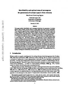
Table 1: Estimation results. The results presented Table 1 show a good improvment in the estimation of parameters p2 , p4 , p7 and delays. The estimation of the other parameters could be improved by using an optimal input design which consists in searching a suitable choice of experimental conditions. Thus a significant increase in accuracy of the parameter estimation can be obtained. The trajectories presented in the figures 1, 2, 3, 4 are obtained by the following way: p = p¯ (full line) and either p = p0 (dotted line) (figures 1, 3) or p = pˆls (dotted line) (figures 2, 4). They show a good trajectory reconstruction and point out the efficiency of the approximated method.

3.3

[2] R. Bellman, K. E. Cooke. ”Differentialdifference equations”, Academic Press, New York (1963). [3] F. Boulier, D. Lazard, F. Ollivier, M. Petitot. ”Computing representations for the radicals of a finitely generated differential ideals” , Technical report, LIFL, Universit´e Lille I. [4] P. Coton. ”Validation de mod`eles de repr´esentation du comportement des a´erodynes en rafales verticales”, Rapport technique IMFL 81/20 (1981). [5] L. Denis-Vidal, G. Joly-Blanchard, C. Noiret, M. Petitot. ”An algorithm to test identifiability of non-linear systems”, Proc. 5th IFAC NOLCOS, St Petersburg, Russia pp 174-178 (2001).

Relation between the approximated system and original system

[6] S, Diop, M. Fliess. ”Nonlinear observability, identifiability, and persistent trajectories”, Proc. 30th CDC, Brighton, pp 714-719 (1991).

The adequacy between the approximate system described previously and the discretized original system has been verified. The obtained trajectories (figures 5, 6 ,7, 8) with the both systems are very closed: in fact they are indistinguishable relatively to the measure error of all states. The trajectories presented in the figures 5, 6, 7, 8 are obtained by the following way: p = pˆls , the discretized original system is given by full line and the approximate system described previously is given by dotted line.

4

[7] C.Jauberthie, L.Belkoura, L.Denis-Vidal, ”Aircraft Parameter and Delay Identifiability”, Proc. 7th ECC, CD Cambridge,(2003). [8] E.R. Kolchin. ”Differential algebra and algebraic groups”, Academic Press, New York. [9] L. Ljung, T. Glad. ”On global identifiability for arbitrary model parametrizations”, Automatica 30-2, pp 265-276 (1994).

Conclusion

[10] M. Malek-Zavarei. ”Time-delay systems, Analysis, Optimization and Applications”, NorthHolland Systems and Control Series, 9, 1987.

This paper presents an approach for the parameter and delay identifiability of aircraft dynamics which consists in a nonlinear and retarded system. In case of unknown delays, the classical methods to test identifiability can’t be applied. By using a practicable input and an approximation of the retarded state based on the Pad´e approximants, a structurally identifiable system is obtained. This

[11] S.I. Nakagiri & M. Yamamoto , ”Unique identification of coefficient matrices, time delays and initial functions of functional differential equations”, J. Math. Syst. Estimation Control, 5, pp 323-344 (1995). 4

3

[12] Y Orlov, L. Belkoura, J.P. Richard, M. Dambrine. ”On identifiability of linear time delay systems”, IEEE Transactions on automatic Control, 47, No.8, pp 1319-1325 (2002).

2

1

0 degree

[13] S.M. Verduyn Lunel, ”Parameter identifiability of differential delay equations”, Int. J. Adapt. Cont. Signal Proc. 15, pp 655-678 (2001).

−1

−2

−3

[14] E. Walter. ”Identifiability of state space models”, Lecture Notes Biomath, 46, (1982).

−4

−5

0

0.1

0.2

0.3

0.4

0.5 time (s)

0.6

0.7

0.8

0.9

1

28.6

Figure 3: Pitch angle reconstruction with p0 .

28.5

28.4

28.3 3 28.2 m/s

2 28.1 1 28 0 degree

27.9

27.8

27.7

−1

−2 0

0.1

0.2

0.3

0.4

0.5 time (s)

0.6

0.7

0.8

0.9

1 −3

Figure 1: Speed reconstruction with p0 .

−4

−5

0

0.1

0.2

0.3

0.4

0.5 time (s)

0.6

0.7

0.8

0.9

1

28.5

Figure 4: Pitch angle reconstruction with pˆls . 28.4

28.3

m/s

28.2

28.1

28

27.9

27.8

0

0.1

0.2

0.3

0.4

0.5 time (s)

0.6

0.7

0.8

0.9

1

Figure 2: Speed reconstruction with pˆls .

5

28.5

20

15

28.4

10 28.3

degree/second

meter/second

5 28.2

28.1

0

−5 28 −10

27.9

27.8

−15

0

0.1

0.2

0.3

0.4

0.5 time (s)

0.6

0.7

0.8

0.9

−20

1

Figure 5: Speed reconstruction (approximate system and discretized original system).

0

0.1

0.2

0.3

0.4

0.5 time (s)

0.6

0.7

0.8

0.9

1

Figure 7: Pitch rate reconstruction (approximate system and discretized original system).

6

3

2 4 1 2

degree

degree

0

0

−1

−2 −2 −3 −4 −4

−6

0

0.1

0.2

0.3

0.4

0.5 time (s)

0.6

0.7

0.8

0.9

−5

1

Figure 6: Angle of attack reconstruction (approximate system and discretized original system).

0

0.1

0.2

0.3

0.4

0.5 time (s)

0.6

0.7

0.8

0.9

1

Figure 8: Pitch angle reconstruction (approximate system and discretized original system).

6