Even if the problem is already well known and solved both in software and in dedicated hardware, a satisfactory solution for FPGA-based real-time convolution is ...
Proceedings of the 24th Euromicro Conference (EUROMICRO 98). pp. 123-130
Image Convolution on FPGAs: the Implementation of a Multi-FPGA FIFO Structure
∗ ✥
Arrigo Benedetti∗✥, Andrea Prati∗, Nello Scarabottolo∗ Dept. of Engineering Sciences, Università di Modena, via Campi, 213, I41100 Modena, Italy phone +39 59 376739, fax +39 59 376799, e-mail {benedett, prati, scarabot}@dsi.unimo.it presently at Computational Vision Laboratory of California Institute of Technology, Pasadena
Abstract In this paper, we present an implementation of a real-time convolver, based on Field Programmable Gate Arrays (FPGA’s) to perform the convolution operations. Main characteristics of the proposed approach are the usage of external memory to implement a FIFO buffer where incoming pixels are stored and the partitioning of the convolution matrix among several FPGA’s, in order to allow data-parallel computation and to increase the size of the convolution kernel.
1. Introduction The work presented in this work is one of the result of a research activity aimed at implementing dedicated architectures for image processing. In particular, the research activity focuses on reconfigurable devices like Field Programmable Gate Arrays (FPGA’s) [1] as the most promising ones in applications where processing speed – typical of dedicated solutions – has to be matched with low-cost, flexible systems capable of performing several different tasks. Among the various algorithms frequently encountered in image processing, we put our attention to 2-D convolution, where a M×N pixels input image has to be convoluted with a K×R kernel to obtain an output image where each pixel depends on a K×R window of neighboring pixels in the input image [2] [3], as shown in Fig. 1. Even if the problem is already well known and solved both in software and in dedicated hardware, a satisfactory solution for FPGA-based real-time convolution is at our knowledge still lacking. To reach such a real-time behavior, it is in fact necessary to process input image pixels – entering the convolution system in the usual raster scan order row-byrow – to ensure an equal rate of output pixels (to avoid unlimited buffering capabilities) and to minimize
Draft version
D00 D01 D02 D03 D04
= pixels already grabbed
D10 D11 D12 D13 D14
= convolution matrix
D20 D21 D22 D23 D24
= central pixel
D30 D31 D32 D33 D34 D40 D41 D42 D43 D44 Figure 1. Convolution of a raster-scan image (K=R=3, M=N=5)
processing latency. In this perspective, a software based solution, where the overall image is stored in RAM memory before starting FPGA computation, seems inadequate for the added latency and the necessity of a large number of memory accesses, possibly exceeding the real-time constraints. A far better approach consists in the implementation of a pipeline processor, where pixels enter the pipeline and produce results as soon as the convolution window has been filled. Referring again to Fig. 1, this means that we need to store (K-1)×N+R pixels and a processing latency – relative to the central pixel of the convolution window – given by R K Lat = + N × 2 2 is introduced. To accomplish this, it is possible to adopt a set of shift registers [4], implementing a FIFO memory able to store the (K-1)×N+R pixels above mentioned. For a n bit per pixel image (i.e., a 2n colors/gray-levels image) this leads itself to n shift registers as shown in Fig. 2, where single flip-flops store pixels belonging to the convolution window (i.e., pixels required to perform the current convolution product) and FIFO blocks store pixels already grabbed and necessary for subsequent convolution
Proceedings of the 24th Euromicro Conference (EUROMICRO 98). pp. 123-130
DK-1,R-1 DK-1,R-2
DK-1,R-3 DK-1,1
FF11 D Q
…
IN
FF12 D Q
DK-1,0
FF1R-1 D Q
DK-2,R-1 DK-2,R-2 FIFO1
IN
FIFO blockOUT dim=N-R+1
FF21 D Q
DK-2,R-3 DK-2,1
FF22 D Q
DK-2,0
FF2R-1
…
D Q
CLK SHIFT1
FIFO2 IN
FIFO blockOUT dim=N-R+1
SHIFT2 D1,R-1
D1,R-2
D1,R-3 D1,1
FF(K-1)1 FF(K-1)2 D Q
D Q
…
D1,0
FF(K-1)R-1 D Q
D0,R-1 FIFO(K-1) IN
FIFO blockOUT dim=N-R+1
D0,R-2
D0,R-3
FF(K)1 FF(K)2 D Q D Q
D0,1
…
D0,0
FF(K) R-1
SHIFTK-1
CLK
OUT
D Q
SHIFTK
Figure 2. Memory structure allowin real-time convolution
products. This approach – quite obvious in dedicated devices – is not well suited to an FPGA implementation. In fact, commercially available FPGA devices contain a limited number of memory elements, since they are constituted by few hundreds of Configurable Logic Blocks (CLB’s), each provided with one or two flip-flops and a configurable logic network. Implementing a memory structure on FPGA’s means using a lot of devices, thus wasting their (re)configuration properties (e.g., with rather large FPGA devices like the Xilinx XC4010E, a 3×3 convolution matrix applied to a 512×512 image using 8 bits per pixels needs (512×2+3)×8=1027×8=8216 flipflops, requiring 11 FPGAs). In fact, previous works (as [5] and [6]) have presented methods for synthesizing FIFO memories using the flip-flops present inside the CLB’s of the Xilinx XC4000 series devices: unfortunately, the number of available CLB’s permits the implementation of FIFO memories far too small for our needs. For this reason, the solution we propose implements the shift registers of Fig. 2 using also external RAM memory interfaced with the convolution FPGA’s. In particular, flip-flops storing pixel values belonging to the convolution window are stored into internal CLB’s, while FIFO blocks storing pixels necessary for subsequent convolution operations are stored into the external RAM memory. The implementation of such a FIFO and its possibilities in terms of speed and kernel size are the main topics of this paper. In Sec. 2, we discuss the requirements of the FIFO memory and the solution that we have implemented for interfacing it with a single FPGA. In Sec. 3, we extend FIFO capabilities to allow parallel processing by several FPGAs, thus relaxing constraints on the convolution matrix dimension. In Sec. 4, an experimental prototype written in VHDL language and implemented in a G800 GigaOps Spectrum board containing 8 Xilinx XC4010E devices is discussed. Finally, possible developments are outlined in Sec. 5.
Draft version
D00 D01 D02 D03 D04
D00 D01 D02 D03 D04
D10 D11 D12 D13 D14 D20 D21 D22 D23 D24
D10 D11 D12 D13 D14 next step
D20 D21 D22 D23 D24
D30 D31 D32 D33 D34
D30 D31 D32 D33 D34
D40 D41 D42 D43 D44
D40 D41 D42 D43 D44
(a)
(b) = pixels already grabbed = convolution matrix = central pixel
Figure 3. Subsequent steps in the convolution of a raster-scan image (K=R=3, M=N=5)
2. The FIFO memory interfaced with a single FPGA To better understand the requirements of the external FIFO memory, it is worth to refer to Fig. 3. In order to minimize the number of external memory accesses necessary to obtain the required FIFO behavior, we propose an apporach based on the following assumptions: • each new pixel entering the convolution system (D23 in Fig. 3-b) is routed both to the FPGA convolver and to the external FIFO memory, where it is stored in a single write cycle; • the K-1 pixels belonging to the convolution “column” of the new pixel (D03 and D13 in Figure 3-b) must be read in K-1 read cycles in order to be routed to the FPGA convolver; • the remaining (R-1)×K pixels (D01, D02, D11, D12, D21 and D22 in Figure 3-b) necessary to perform the convolution are stored inside the FPGA. Summarizing, for each new pixel coming from the video signal source via the frame grabber, 1 memory write and K-1 memory reads must be performed to correctly feed the FPGA convolver.
Proceedings of the 24th Euromicro Conference (EUROMICRO 98). pp. 123-130
External RAM 0000 D01
D02
D00
0001
D00
0002 D Q
D Q
D Q
D Q
D Q
D Q
0003 0004
SHIFT1
SHIFT2
0005
SHIFT3
0006 0007
after the first R-1=2 pixels
0008
(a)
External RAM counter D03
D04
D02
00000 D00 D00 000 0001 D01 0002 D02
D Q
D Q
D Q
D Q
D Q
D Q
0003 0004
SHIFT1
SHIFT2
0005
SHIFT3
0006 0007
after N-R+1=3 more pixels
(b)
0008
counterrd(1) D13
D14
D12
D03
D04
D02
External RAM 00000 D00 D00 000 0001 D01 0002 D02
D Q
D Q
D Q
D Q
D Q
D Q
counterwr
0003 D03 0004 D04
SHIFT1
SHIFT2
0005 D10
SHIFT3
0006 D11 0007 D12
after N=5 more pixels
(c)
0008
External RAM counterrd(0) D21
D22
D20
D11
D12
D10
D01
D02
D00
D14 00000 D00 D00 000 0001 D01 D20 0002 D02
D Q
D Q
D Q
D Q
D Q
D Q
0003 D03 0004 D04
SHIFT1
SHIFT2
SHIFT3
counterrd(1)
0005 D10 0006 D11 0007 D12
after N-R+1=3 more pixels counterwr
(d) Figure 4. Behavior of the external FIFO (N=M=5, K=R=3)
Draft version
0008 D13
Proceedings of the 24th Euromicro Conference (EUROMICRO 98). pp. 123-130
This has been accomplished in the FPGA system by implementing the FIFO memory in a circular buffer stored in RAM, based on the following elements: 1. The input/output clock signal, here called video clock, which synchronizes frame grabber and video encoder operations. During each cycle of clock, a new pixel enters the convolver and a new complete convolution takes place. 2. A convolution clock, whose frequency fconv is K times higher than the frequency fplay of the play clock. During each cycle of the convolution clock, a memory access (either read or write) to the external FIFO is performed. 3. A write pointer counterwr, stored inside the FPGA convolver is used to address the first free location inside the external FIFO, where the incoming pixel has to be stored. 4. K-1 read pointers counterrd(i), also implemented inside the FPGA are used to address the locations of the pixels to be read from the external FIFO to complete the computation of the convolution window. Using the above elements, the external FIFO, requiring a memory able of accommodating at least (K-2)×N+(N-R+1)+1=(K-1)×N-R+2 pixels, is obtained
as summarized in Fig. 4, where a 3×3 convolution window and a 5×5 input image are assumed. Before starting to fill the FIFO, R-1 pixels have to be shifted into the SHIFT1 register (Fig. 4.(a)). The next NR+1 pixels are stored in the FIFO denoted FIFO1 in Fig. 2, filling it until counterwr reaches location 0002 (Fig. 4.(b)). At this time counterrd(1) is enabled and starts to address data from FIFO1 and to shift them into SHIFT2. After N additional pixels (i.e., a full image row has been read) counterrd(0) is enabled in turn and begins to store data in SHIFT3 The situation is shown in Fig. 4.(c). After N-R+1 additional pixels, the first convolution window is available and the FPGA starts the computation using counterrd(0) and counterrd(1) to fetch D02 and D12 from the FIFO (Fig. 4.(d)). It should be noticed that this approach poses the following limits on the dimension of the convolution matrix: 1) a first limit derives from the maximum frequency allowed for the convolution clock, used to access the external RAM memory to fetch the next “column” of pixels. This limit affects then the maximum number of rows (thus the value of K) in the convolution matrix: referring to the 8.33 MHz of the video clock (adopted by the european PAL video standard) and Input
delay unit
FIFOn-1 FIFOn
…
Calculationn
Draft version
…
Calculationn-1 FPGAn
Figure 5. Multi-FPGA architectural schema
delay unit (n-2)xk1xN
…
FPGAn-1
FPGA0
FIFO2
…
FIFO block dim= k 2 ∗ N
(n-1)xk1xN
delay unit k1xN
…
FPGA2
Calculation2
…
Output
Calculation: second level
FIFO block dim= [(n − 3) ∗ k1 + k 2 ] ∗ N
…
FPGA1
FIFO1
dim= [(n − 2 ) ∗ k1 + k 2 ]∗ N
Calculation1
FIFO block
Proceedings of the 24th Euromicro Conference (EUROMICRO 98). pp. 123-130
using 20 nsec access time RAM (i.e.,50 MHz maximum fconv), this results in a convolution matrix of at most 6 rows; 2) a second limit derives from the capacity of the FPGA convolver, that, even in case of particularly favorable convolution matrices (containing only 0s, 1s and power-of-2 coefficients, thus requiring only logical operations and shifts - e.g. Sobel, Prewitt and Laplace matrices [2] - which can be implemented using few CLBs), has to store inside the internal flip-flops the K×R pixels to be handled. This limit affects then the overall dimension of the convolution matrix. It is easier shown that the most critical parameter in terms of capability of handling large convolution kernels is the number K of rows; moreover, it can be noticed that, for a given “area” of the convolution matrix, it is more convenient to minimize K and maximize R in order to relax clock constraints. On the basis of the above considerations, we have devised a multi-FPGA structure that is presented in the next section.
3. Multi-FPGA solution When several FPGA devices are available, the most convenient way of partitioning computation among them is represented in Fig. 5: n FPGAs are used to process in parallel n different portions of the convolution window, and an additional FPGA (the 0-th one in Figure 5) merges intermediate results performing (usually) simple sum operations. This would mean to subdivide the K×R convolution matrix into n sub-matrices of size k×r, where the following relations hold: K R k= , r= , p×q=n . (1) p q A great deal of work exist about partitioning FPGA designs (e.g., [7], [8] and [9]), however, given the considerations expressed in previous section, the best choice for the convolution matrix subdivision in our case is given by p=n , q =1 , which means a set of horizontal “stripes”. It must be noticed however that the second level FIFO blocks shown in Fig. 5 have to be included to ensure that the results of each single convolution stripe reach FPGA0 aligned in time. These FIFO’s introduce the need of two additional accesses to external RAM: one to write the input and one to read the output. In other words, all the FPGA’s but the last one must use two cycles of the convolution clock to access the second level FIFO’s, which implies two less accesses to their first-level FIFO, which contains the pixel values to be multiplied. Since the number of allowed accesses to first-level FIFO’s is the upper limit to the number of rows in each stripe, and since the last FPGA does not need a second level FIFO, the best subdivision of the convolution matrix
Draft version
can be obtained as follows. Referring to Fig. 5, we see that the original K rows must be partiotioned into p stripes of R columns: one stripe of k2 rows and p-1 stripes of k1 rows. For previous considerations, k2=k1+2. Obviously, to correctly partition the original K rows, k1×(n-1)+k2=K must hold. From this equation we can show that K-2 K-2 k1 = k2 = +2 . (2) , n n Delay units in Fig. 5 allow each FPGA to obtain its own stripe of data. Besides the advantages already discussed, this approach allows to optimally map the convolution matrix into n FPGAs provided that: (K-2) mod n = 0 without any other constraint upon R. To estimate the effectiveness of such approach, let us revise the practical example made at the end of previous section. For a 20 nsec access time RAM to be used in a system working with the european PAL video standard, we have: • fplay = 8.33 MHz • maximum fconv = 50 MHz • maximum number k of accesses to external RAM in a 50 video clock cycle: =6 8.33 • maximum K dimension of the convolution window: (n-1)×(6-2)+6=4n+2 For a system with n=8 FPGAs, using only square kernels, this means a 34×34 upper limit to the kernel dimension. If we remove the choice of square matrices, it is possible to furtherly increase R up to the space limit given by the number of available CLB’s.
4. Prototypal implementation In this section, we present a VHDL [10] implementation of the multi-FPGA structure, discussed in previous section, on a multi-FPGA board designed for rapid prototyping [11]. To this purpose, we first describe the main characteristics of the prototyping board, with particular reference to the ones limiting the degrees of freedom in mapping computation and data paths onto the available FPGA’s. Then, we show our solution and we evaluate the results.
4.1 Prototypal board The prototyping board we used is the GigaOps G800 Spectrum board [12] , schematically shown in Fig. 6. In Fig. 6 it is possible to notice the main blocks of this system. • The actual computation is performed by pairs of Xilinx XC4010E FPGA’s, connected in modules
Proceedings of the 24th Euromicro Conference (EUROMICRO 98). pp. 123-130
Figure 6. Block diagram of the GigaOps G800 board
called XMOD’s: in Fig. 6, four modules (MOD0 thru MOD3) are shown. These FPGAs are named YPGA and XPGA (from the name of the bus they are connected with). Both these FPGAs have two memory ports: one connected only to a 2 MBytes DRAM and one connected both to a 2 MBytes DRAM and to a 128 KBytes SRAM device. XPGA and YPGA communicate through a bus switch on the first memory port. This switch works on two virtual busses: a 16-bit data bus and a 10-bit address bus. It is important to stress that only YPGA’s are connected to YBUS, i.e. to the input/output data bus. • A module called SCVIDMOD (S-VIDEO, COMPOSITE, VIDEO MODULE), that decodes/encodes video signals (PAL or NTSC). This module interfaces to YBUS for data input and output. • An input FPGA (here called VLPGA) connected to the VESA local bus of the PC hosting the board. The VLPGA is interfaced with the HBUS and the YBUS. It contains all the registers needed for correct board operation (e.g., the CLKMODE register, that sets frequencies of the clocks distributed on the board). • An output FPGA (here called VMC) connected to SCVIDMOD. This is an additional FPGA, directly interfaced with the video output and the XBUS. • Three main busses that allow connections among the various blocks of the board. These busses are: ¾ YBUS, a 32-bit I/O bus connected with VLPGA, VMC and the YPGA’s of the XMOD’s. ¾ HBUS, a 16-bit bus used to configure and to load the FPGA’s. ¾ XBUS, a 64-bit bus normally used as four 16-bit data busses. Each of these busses is connected only to the XPGAs of the and to VMC. The main data path of our application is the following: pixels generated by the video decoder are passed through the YBUS both to VLPGA and to the YPGA’s of the XMOD’s. These modules process data and pass the results either to the VMC FPGA through YBUS or to the XPGA’s through the bus switches. In the latter case, the XPGA’s can perform a further computation or simply pass the results to the VMC FPGA through the 64-bit XBUS. In
Draft version
both cases, the VMC FPGA outputs the results of its processing upon data coming from the XBUS or YBUS.
4.2 The convolver prototype A first characteristic that limits the degrees of freedom of this system is the kind of access to input/output data. In fact, XPGA’s are not connected to the YBUS, therefore they receive data to be processed only through the YPGA’s. This affects the effectiveness of the implementation: in particular, it makes more difficult to handle a multi-FPGA architecture that uses also XPGAs than an architecture using only YPGAs. Another limit is constituted by the busses that interconnect XPGA’s with YPGA’s. These busses are also used to access to the 2 MBytes DRAM’s. It is then extremely difficult to manage and to synchronize both connections with XPGA and with DRAM. It is easy to note that the above restrictions make very hard and not effective to use both XPGAs and YPGAs to map computations. On the contrary, XPGAs become useful to implement the second level FIFOs of Figure 5: this approach allows, in fact, to relax the constraints on the maximum number of accesses defined in the previous section. Thus, we can perform on each YPGA’s a convolution with a k×r kernel. Referring to the above considerations we decided to implement our prototype using only YPGA’s to perform convolution. In particular, since our own device has four XMOD’s, our multi-FPGA convolver uses the 4 YPGAs to map computation and the 4 XPGA’s to simply implement second level FIFO’s. Some additional considerations are needed to completely understand our prototype. Since every memory access requires first to present the memory address and to assert control signals (like memory read and memory write) then to deactivate these control signals before the next memory access, it is necessary to identify two timing events for starting and ending each memory access.
Proceedings of the 24th Euromicro Conference (EUROMICRO 98). pp. 123-130
External RAM1 0000 D01
D02 D Q
D00 D Q
D Q
SHIFT1
D Q
D Q
SHIFT2
D Q
SHIFT3
after the first R-1=2 pixels (a)
External RAM2
D00
0000
0001
0001
0002
0002
0003
0003
0004
0004
0005
0005
0006
0006
0007
0007
0008
0008
External RAM1 0000
D D0001
External RAM2 counterwr
0001 D03
D04 D Q
D02 D Q
D Q
SHIFT1
D Q
D Q
SHIFT2
D Q
SHIFT3
after N-R+1=3 more pixels
(b)
D13 D Q
D12
D03
D04
D Q
D Q
SHIFT1
D02 D Q
D Q
SHIFT2
(c)
D Q
SHIFT3
after N=5 more pixels
D21 D Q
D20 D Q
D11
D12 D Q
D10 D Q
D01
D02 D Q
D00 D Q
SHIFT2
SHIFT3
after N-R+1=3 more pixels
(d)
0001 0002 0003
0004
0004
0005
0005
0006
0006
0007
0007
0008
0008
0000
DD0001
0001
D03
0002
D10
0003
D12
External RAM2 counterrd(1)
counterwr
D00
0000
D02
0001
D04
0002
D11
0003
0004
0004
0005
0005
0006
0006
0007
0007
0008
0008
0000
DD0001
0001
External RAM2 counterrd(0)
D00
0000
D03
D02
0001
0002
D10
D04
0002
0003
D12
D11
0003
0004
D14
D13
0004
D20
0005
0005 SHIFT1
D02
0003
External RAM1
D22
0000
0002
External RAM1
D14
D00
counterrd(1)
counterwr
0006
0006
0007
0007
0008
0008
Figure 7. Behavior of the external FIFO implemented on dual-port memory (K=R=3, N=M=5)
Draft version
Proceedings of the 24th Euromicro Conference (EUROMICRO 98). pp. 123-130
Due to board and memory characteristics, this poses an additional limitation: the maximum-frequency clock available (33.33 MHz: four times the PAL video standard fplay) generates an event (either a rising edge or a falling edge) every 15 nsecs. This does not match the 30 nsec access time EDO DRAM access time (present on recent versions of the G800 board), nor the 60 nsec access time DRAM (present on our prototype board), thus implying to reduce the performance by using only some edges of the clock waveform. To avoid this problem, strictly related to the type of board and memory chips available, we exploited the second RAM port present on the X210 modules, to perform two memory accesses at a time. Clearly, we must properly alternate memory writes and reads on the two ports. In Fig. 7 an example is reported. With this approach, the FPGA’s make two memory accesses per cycle of video clock to each of the two RAM banks available, allowing to reach an upper limit of a 16×16 convolution matrix with 30 nsec access time EDO DRAM and an upper limit of an 8×8 kernel with a 60 nsec access time DRAM. In fact, in this case, FPGA’s can perform only one memory access per cycle of play clock to each of the two banks.
5. Conclusion and future work In this paper, we have presented the architecture of a real-time convolver implemented by using FPGA’s. In particular we have focused on the constraints that limit the maximum matrix dimension, which is directly related to the effectiveness of convolver. We have described a possible solution to relax these constraints, based on data parallelism. In our prototype, we started testing the multi-FPGA architecture with several 3×3 convolution matrices, e.g., Sobel, Prewitt, Kirsch, Laplace and Cantoni operators [2] [3]. The limited dimension of these convolution matrices allowed us to perform convolution row-by-row on three different YPGA’s, without requiring first-level FIFO memories, thus avoiding the two external memory accesses discussed in the previous section. Second level FIFO’s and final calculations are performed by the XPGA’s and the VMC, respectively. This choice led to meet the real-time constraints also in our G800 prototypal board: in fact, even with a 60 nsec access time DRAM, the dual port used by the XPGAs allows to implement second-level FIFOs. The next step will be the implementation of an 8×8 convolution matrix, spreading over 4 YPGAs the 8 convolution rows and using again the XPGAs for second level FIFO’s. The fact that each YPGA has to process two convolution rows implies the implementation of first level FIFO’s, requiring two external memory accesses per video clock as in the case of the XPGAs (thus still viable on our G800 board).
Draft version
Larger convolution matrices can be considered only using new versions of the G800 board, featuring faster DRAMs. A more significant evolution of the present architecture is the implementation of a series of convolutions. In fact, the experiences on the 3×3 matrices showed that both YPGA and XPGA are underutilized (25% to 30% of CLBs not used). It seems then feasible to use both YPGA and XPGA for computation and FIFO management, thus allowing to perform, on the same image, two subsequent convolutions. This can be useful to have an initial image filtering (to enhance signal-to-noise ratio) or to perform edge detection and computation of the brightness gradient (as required, for instance, in the Hough transform).
References [1] D. Buell (editor). Splash 2 : “FPGA’s in a Custom Computing Machine”. IEEE Computer Society Press, 1996 [2] Virginio Cantoni, Stefano Levialdi, “La visione delle macchine – Tecniche e strumenti per l’elaborazione di immagini e il riconoscimento di forme”, Tecniche Nuove, Milano, 1990 [3] Vito Cappellini, “Elaborazione numerica delle immagini”, Boringhieri, Torino, 1985 [4] The Programmable Logic Data Book. Xilinx, San Jose, CA, 1996 [5] Peter Alfke, “Synchronous and Asynchronous FIFO Designs”. Xilinx Application Note XAPP 051, September 1996, Version 2.0 [6] Jazi Eko Istiyanto, “The Formation of Super-Cliques in the Behavioural Synthesis of FIFO RAMs”, Tech Report, Gadjah Mada University [7] P.Athanas and L. Abbott. “Addressing the Computational Requirements of Image Processing with a Custom Computing Machine: An Overview”. In Proceedings of the 2nd Workshop on Reconfigurable Architecture, Santa Barbara, CA, April 1995 [8] Stephen L. Wasson, “FPGA Design: Early Implications In Partitioning”, Integrated System Design magazine, February 1997 [9] S. Hauck, Multi-FPGA Systems PhD thesis, Department of Computer Science, University of Washington, Sep 1995 [10] IEEE Standard VHDL Language Reference Manual. IEEE Standards [11] FPGA Compiler User Guide v3.5. Synopsys, Mountain View (USA), Sep 1996 [12] Giga Operations Spectrum Documentation. Giga Operations Corporation, Berkley, CA, 1995