In contrast, Convolution Shadow Maps (CSM) enable tri-linear filtering of shadows and thereby ... dard for rendering shadows in movie productions and video.
Eurographics Symposium on Rendering (2007) Jan Kautz and Sumanta Pattanaik (Editors)
Convolution Shadow Maps Thomas Annen1 1 MPI
Informatik Germany
Tom Mertens2
Philippe Bekaert2
Hans-Peter Seidel1
2 Hasselt University — EDM transationale Universiteit Limburg, Belgium
Percentage Closer Filtering
3 University
Jan Kautz3 College London UK
CSM with 7x7 blur and mip-mapping
Figure 1: Standard percentage closer filtering does not support tri-linear filtering and suffers from severe aliasing artifacts during minification. In contrast, Convolution Shadow Maps (CSM) enable tri-linear filtering of shadows and thereby achieve effective screen-space anti-aliasing. Additional convolution can hide shadow map discretization artifacts. Abstract We present Convolution Shadow Maps, a novel shadow representation that affords efficient arbitrary linear filtering of shadows. Traditional shadow mapping is inherently non-linear w.r.t. the stored depth values, due to the binary shadow test. We linearize the problem by approximating shadow test as a weighted summation of basis terms. We demonstrate the usefulness of this representation, and show that hardware-accelerated anti-aliasing techniques, such as tri-linear filtering, can be applied naturally to Convolution Shadow Maps. Our approach can be implemented very efficiently in current generation graphics hardware, and offers real-time frame rates. Categories and Subject Descriptors (according to ACM CCS): I.3.3 [Computer Graphics]: Picture/Image Generation–Bitmap and Frame Buffer Operations; I.3.7 [Computer Graphics]: Three-Dimensional Graphics and Realism–Color, Shading, Shadowing and Texture
1. Introduction Shadow Mapping [Wil78] has grown into a de facto standard for rendering shadows in movie productions and video games. As it is a purely image-based approach, Shadow Mapping is robust against increased scene complexity, and translates well to graphics hardware. Shadow Maps are constructed by rasterizing a depth image from the light source’s c The Eurographics Association 2007. �
vantage point, thereby recording the distance to the closest surfaces. Any scene point can be projected into the light’s view to retrieve the corresponding blocker distance. If this distance is smaller than the actual distance to the light source, the point is in shadow. Unfortunately, Shadow Mapping has its problems. Since the blockers are discretized, aliasing artifacts like jagged
T. Annen, T. Mertens, P. Bekaert, H.-P. Seidel & J. Kautz / Convolution Shadow Maps
edges can occur. Novel variants of Shadow Mapping have been introduced to alleviate discretization [FFB01, SD02, SCH03], but these methods do not offer a solution for screen-space aliasing. In particular, detailed shadows may give rise to Moiré patterns when viewed from far, especially as geometric complexity increases. For texture mapping, screen-space aliasing can be dealt with efficiently through high-quality filtering, which is commonly found on graphics hardware. Unfortunately, filtering the Shadow Map’s depth values does not produce the desired solution, as one wants to filter the results of the shadow test. Reeves et al. [RSC87] were the first to switch the order of filtering and testing. This led to the Percentage Closer Filtering (PCF) algorithm, and is available on current graphics hardware. PCF performs filtering by taking multiple shadow samples and averaging them together. Unfortunately, it cannot support prefiltering, and is therefore limited to small filter kernels for efficiency reasons. Mip-mapping is an efficient version of prefiltering [Wil83], which fetches pre-convolved texture samples from an image pyramid and allows for effective antialiasing. Since the shadow test depends on the distance between the query point and the light source, which can change at run-time, this kind of pre-filtering is not possible. However, Variance Shadow Mapping [DL06] showed that a statistical estimate of a convolved depth test can be computed at run-time allowing for filtered shadows. Unfortunately, this estimate is biased and leads to disturbing high-frequency artifacts for scenes with high depth complexity. This paper introduces the Convolution Shadow Map, a novel Shadow Mapping variant that permits filtering of Shadow Maps with arbitrary convolution filters. Convolution Shadow Maps support mip-mapping, which enables high quality tri-linear and anisotropic filtering, in order to prevent screen-space aliasing. In addition, we can directly blur the Convolution Shadow Map in order to soften shadow borders, which is particularly useful for concealing discretization artifacts and simulating penumbrae. Key to our approach is that we encode a binary visibility function instead of explicitly storing depth values at each pixel. These functions are approximated with a basis function expansion, which allows a “linearization” of the shadow test. Compared to Variance Shadow Maps [DL06], our approach is unbiased and can deal with arbitrary depth complexity. We demonstrate that Convolution Shadow Maps can be efficiently implemented on current graphics hardware.
2. Related Work Shadows. Ray tracing [Whi79] naturally takes care of shadowing, but is currently not feasible on commodity hardware. Shadow Volumes [Cro77] offer crisp shadows in a rasterization-based renderer, but they are strongly dependent on geometric complexity. Shadow Mapping [Wil78] is a purely image-based approach, and is therefore less sensi-
tive to geometric complexity. This paper proposes a novel way of filtering Shadow Maps for anti-aliasing. Anti-Aliasing. After its introduction, a lot of effort has focused on tackling the inherent aliasing problem with Shadow Mapping. First, efficient filtering techniques similar to texture filtering [Hec89] have been investigated. Reeves et al. [RSC87] observed that shadows should be anti-aliased by filtering Shadow Map pixels after the depth test. This idea was later implemented in graphics hardware. Unfortunately, high quality texture map filtering based on mipmapping [Wil83] is not directly applicable since the result of the filter cannot be precomputed. Deep Shadow Mapping [LV00] precomputes the aggregate result of binary shadow tests within each texel for excessively complex scenes like hair, yielding a continuous visibility function for each texel, which can be queried at render-time. Our technique bears some similarity to Deep Shadow Maps, since we also store a visibility function. However, we are only interested in using binary visibility functions, and applying spatial convolution instead of intra-pixel averaging. In a recent effort, Donnelly and Lauritzen [DL06] introduced Variance Shadow Maps for rendering filtered shadows. They compute only a statistical upper bound to the result of the filter, which yields noticeable artifacts (“light leaking”). The upper bound becomes an equality only when the receiver and occluders are planar and parallel, and therefore the artifacts quickly worsen as depth complexity increases (see Fig. 9). Our method requires less stringent assumptions, and even though it is also approximate, it converges to the exact solution instead of an upper bound. Researchers have also tried to tackle aliasing by extending the Shadow Map representation. Adaptive Shadow Mapping [FFB01] hierarchically refines shadow borders. Perspective Shadow Mapping [SD02] computes the Shadow Map in a perspectively distorted space which yields a better sampling distribution with respect to the vantage point. It is possible to find an optimal distribution [AL04], but unfortunately it is irregular and therefore does not map well to current graphics hardware. Shadow Silhouette Maps [SCH03] embed silhouettes for rendering perfectly hard shadows, but cannot deal with every possible configuration of shadow boundaries. Combinations between Shadow Mapping and Shadow Volumes are also possible [CD04]. These technique offer ways for rendering sharper shadows, but they do not address aliasing in screen-space. Our method could be used in conjunction with some of these techniques (e.g., [SD02]). Soft Shadows. Accurate real-time display of soft shadows due to extended light sources, is a topic of ongoing research. See Guennebaud et al. [GBP06] and references therein for recent work, and Hasenfratz et al. [HLHS03] for a survey. Instead of physically-based computation, rendering inaccurate but visually plausible soft shadows in order to lessen computational effort, is a viable alternative. Chan and Durand [CD03] and Wyman and Hansen [WH03] create plausic The Eurographics Association 2007. �
z(p2)
d(x1) = z(p1)
T. Annen, T. Mertens, P. Bekaert, H.-P. Seidel & J. Kautz / Convolution Shadow Maps
d(x2)
p1 p2
p
p-q
blocker
y x1
x2
(a)
x
y
(b)
Figure 2: Fig. (a) illustrates shadow mapping. Point x1 is lit, while point x2 is in shadow. Fig. (b) depicts convolution using a filter kernel w. Filtering for a point x is performed in shadow map space around point p. See text for more information on q and y. ble penumbrae, but overestimate umbra size and also require costly silhouette information. Brabec and Seidel [BS02] attenuate light rays near blockers to reproduce the outward decay in visibility with respect to the umbra region, but rely on a costly neighborhood search in the depth map. Our technique follows up on this line of work: we provide a way to mimic soft shadows by applying a large convolution filter. This effectively creates a soft penumbra, but its width is constant with respect to the projected Shadow Map size. This refrains us, for instance, from creating hard contact shadows where blocker and receiver meet. However, our approach is cheaper compared to previous techniques. Our method is similar to Soler and Sillion’s convolution method [SS98], which convolves binary blocker images. We extend their approach to depth maps [Wil78], but we are currently limited by a constant-sized convolution kernel. 3. Convolution Shadow Maps We first formally introduce Shadow Mapping, before we go on to Convolution Shadow Maps. Let x ∈ R3 be the worldspace position of a pixel. We will use boldface characters to indicate positions; other variables are scalars. Point p ∈ R2 represents the position of a shadow map pixel, which is obtained via a surjective mapping T : R3 → R2 between worldspace and shadow map space, such that p = T (x). This mapping basically warps a pixel into Shadow Map space via a perspective projection. The Shadow Map itself encodes a function z(p), that represents the depth of the blocker that is closest to the light source for each p. A pixel with worldspace position x is considered in shadow when d(x) > z(p), with d(x) being the depth of x (again, with respect to the light source). See Fig. 2. We now formally define a shadow function s, that basically encodes the shadow test: � � s(x) := f d(x), z(p) (1) where f (d, z) is a binary function that returns 0 if d > z and 1 otherwise. c The Eurographics Association 2007. �
Convolution In order to have anti-aliased shadows, we need to filter the shadow function s(x) (e.g., using a low pass filter). Generally speaking, a convolution (or linear filtering) operation on a function g with kernel w supported over a neighborhood N , is defined as: � � (2) w ∗ g (p) := ∑ w(q)g(p − q) q∈N
Let us now try to convolve the shadow function s(x), and denote the result as s f (x): � � (3) s f (x) = ∑ w(q) f d(y), z(p − q) q∈N
Even though s f is formulated in terms of x, the actual convolution happens in Shadow Map space, i.e. over variable p. Eq. 3 contains a new variable y, which is informally defined as the point that lies near x, such that T (y) = p − q. Unfortunately, there is no unique y = T −1 (p − q), because T is not invertible, see Fig. 2b. In order to arrive at a mathematically sound formulation of Shadow Map convolution, we need to assume that d(y) ≈ d(x), so that we can write: � � s f (x) = ∑ w(q) f d(x), z(p − q) q∈N
� � �� = w ∗ f d(x), z (p)
(4)
This assumption d(y) ≈ d(x) basically states that d(x) is a representative distance for the neighborhood N , which is only correct for a planar receiver, parallel to the Shadow Map’s image plane. Note that a similar approximation is made for percentage closer filtering [RSC87], and in Soler et al.’s work [SS98]. It is important to see that we cannot directly apply convolution to z(p), because f is nonlinear with respect to its arguments. In other words: � � �� � � (5) w ∗ f d(x), z (p) �= f d(x), (w ∗ z)(p) This explains why regular texture filtering cannot be applied to z(p) (i.e., the Shadow Map): filtering z(p)-values is not equivalent to filtering the result of the shadow test. It is possible however, to carry out the summation in Eq. 5 directly at runtime [RSC87]. However, our goal is to apply pre-filtering. In other words, to apply a filter before it is actually used. This would enable efficient separable filtering, and more importantly, to employ mip-mapping. To achieve this, we transform the z-values such that the shadow test can be written as a sum. This will allow us to “linearize” the depth test. Let us therefore expand f (d, z) as follows: f (d, z) =
∞
∑ ai (d)Bi (z)
(6)
i=1
Here, Bi are basis functions in terms of z, which we will concretely define in Section 3.1. Each basis is weighted by
T. Annen, T. Mertens, P. Bekaert, H.-P. Seidel & J. Kautz / Convolution Shadow Maps
corresponding coefficients ai depending on d. The expansion has to be truncated in practice to some truncation order N (and we silently omit the ≈-relation in the following formulas). We see that the expansion does not yield a direct linear dependence on z, but it is linear with respect to the basis set Bi=1...N . In order to apply this expansion in practice, we convert the Shadow Map to “basis images” � by�applying each basis function to the Shadow Map: Bi z(p) . Consequently, the shadow function in Eq. 1 can be translated to linear combination of these basis images: s(x) =
� � � � ∑ ai d(x) Bi z(p) N
(7)
function, in order to make it periodic (a requirement to apply a Fourier series approximation). Let S(t) be a square wave function with period 2. For t ∈ (−1, 1) we have H(t) = 1 1 2 + 2 S(t). For this particular case of S(t), the (truncated) Fourier series expansion yields: S(t) ≈
N � � � � = w ∗ ∑ ai d(x) Bi (p)
f (d, z) ≈
=
N
∑ ai
�
�� � d(x) w ∗ Bi (p)
sin(a − b) = sin(a) cos(b) − cos(a) sin(b)
3.1. Fourier Expansion We expand the shadowing function f according to Equation 6 using a Fourier series. In general, we can decompose any periodic function g(t) as an infinite sum of waves: ∞ � 2πn 2πn � 1 t) + bn sin( t) , g(t) = a0 + ∑ an cos( 2 T T n=1
(9)
where the coefficients an and bn are obtained by integrating the cosine and sine basis functions against g, respectively. This is the standard Fourier series and will be used to represent the shadowing function. f is a function in terms of 2 variables, but it can be expressed with as the Heaviside step (or the “unit step”) function, H(t), as follows: f (d, z) = H(d − z). Let us first focus on expanding H(t). We represent it using a square wave
M 1 1 cos(ck d) sin(ck z) +2 ∑ 2 c k=1 k M
(12)
(13)
1 −2 ∑ sin(ck d) cos(ck z) c k=1 k
i=1
The success of our technique will obviously depend on the chosen expansion. As detailed in the next section, we choose the Fourier series. For clarity, we note that the Fourier expansion will not be used for applying the convolution theorem to �perform � spatial filtering; convolution of the basis images Bi z(p) will be done explicitly.
(11)
Now we have:
(8)
The last equation is the key observation in our paper: any convolution operation on the shadow function � is equivalent � to convolving the individual basis images Bi z(p) . It is important to see that in order to reach Eq. 8, each term in the expansion (Eq. 6) had to be separable with respect to variables d and z. Decoupling d(x) from z(p) is important, be� � cause it enables us to convolve the images Bi z(p) before the shadow test.
M � � 1 1 sin ck (d − z)) , +2 ∑ 2 c k=1 k
with ck = π(2k −1). We convert the previous summation into a form similar to Eq. 6 using the trigonometric identity
f (d, z) ≈
i=1
(10)
Now, returning to f we have:
i=1
To see why this is useful, we fill in the expansion from Eq. 7 in the convolution in Eq. 4: � � �� s f (x) = w ∗ f d(x), z (p)
� � 4 M 1 sin (2k − 1)πt ∑ π k=1 2k − 1
We see that Eq. 13 complies with Eq. 6, and have separable terms w.r.t. d and z: a(2k−1) (d) = B(2k−1) (z) =
2 ck
cos(ck d), a(2k) (d) = sin(ck z), B(2k) (z) =
−2 ck
sin(ck d) (14) cos(ck z)
with k = 1 . . . M (note that N = 2M in Eq. 6). We add the constant term 12 separately. 3.2. Discussion of Fourier Expansion We opted for the Fourier expansion for two reasons. First, it is shift-invariant w.r.t. d and z, which is a general property of the Fourier transform (cf. rotational invariance of Spherical Harmonics [SKS02]). Intuitively speaking, this enables us to “move” the Heaviside step around without any loss in precision. In fact, this can be done by independently changing d and z, while keeping the approximation error due to truncation constant. The second reason is that the basis functions (sine and cosine waves) are bounded: they always map to the interval [−1, 1]. This affords a fixed point representation, which we can even quantize to 8 bits in practice. The Fourier series does not come without disadvantages. First, as with any Fourier representation, it is prone to ringing. Second, the Fourier expansion smoothes the step function, which can result in incorrect shadowing if not handled. We deal with both problems as shown the following subsections. 3.2.1. Ringing A Fourier expansion potentially suffers from ringing (Gibbs phenomenon), particularly when the expansion is truncated to a small number of terms M. We � effect by at� reduce this tenuating each k-th term by exp − α( Mk )2 . Parameter α c The Eurographics Association 2007. �
T. Annen, T. Mertens, P. Bekaert, H.-P. Seidel & J. Kautz / Convolution Shadow Maps 1.2
1.2 M=1 M=4 M = 16
Alpha = 1.0 1 CSM Shadow Test
CSM Shadow Test
1 0.8 0.6 0.4 0.2 0
0.8 0.6 0.4 0.2 0
−0.2 −0.5
0 (d−z)
−0.2 −0.2
0.5
(a) Reconstruction
−0.1
0 (d−z)
1.2
0.2
2.5 Offset = −0.032
1
Scaling by 2.0
2 CSM Shadow Test
CSM Shadow Test
0.1
(b) Ringing Suppression
0.8 0.6 0.4 0.2
1 0.5
0
0
−0.2 −0.2
−0.5 −0.2
−0.1
0 (d−z)
0.1
0.2
(c) Offset
(a) Scaling
−0.1
0 (d−z)
0.1
0.2
(d) Scaling
Figure 3: Reconstruction and various tradeoffs. The x-axis encodes the difference (d − z) along a shadow ray (lookup). (a) illustrates the conflict of increasing M to achieve a more reliable shadow test and introducing high frequencies noticeable as ringing artifacts. (b) shows the impact of attenuation to suppress ringing as the red turns into the blue signal. Plots in (c) and (d) show methods to enhance the shadow test. In (c) an offset is applied to d before reconstruction, which prevents incorrect darkening of lit areas. (d) shows how scaling makes the transition steeper and how it also prevents incorrect darkening. Please compare (c) and (d) with the results in Fig. 4. Note that for illustration purposes the range has been scaled to emphasize the effects. controls the attenuation strength (α = 0 leaves the series unchanged). The magnitude of the high frequencies is always reduced more, while the low frequencies remain almost the same. This incurs an important tradeoff: reducing ringing also means that the reconstructed Heaviside step becomes less steep (see Fig. 3). 3.2.2. Offsetting and Scaling The Fourier expansion of the step function introduces a smooth transition, which is especially obvious with loworder expansions M, see Fig. 3(a). This means that for lit surfaces, where (d − z) ≈ 0, the shadow function f (d, z) evaluates to 0.5. This is undesirable, as all lit surfaces would be 50% shadowed. We can correct this, by offsetting the expansion of the Heaviside step, see Fig. 3(c). After offsetting, f (d, z) goes through 1 for (d − z) ≈ 0, which results in correctly lit surfaces. The shift-invariance property of the Fourier expansion allows us to formulate a constant offset, which only depends on the truncation order and can thus be applied at every pixel. Of course, offsetting makes the transition from unshadowed to shadowed more obvious near contact points. Scaling the expansion by 2.0 makes the transition steeper c The Eurographics Association 2007. �
(b) Offset
1.5
Figure 4: Difference of scaling f or subtracting an offset from d. (a) illustrates that scaling f sharpens the transition but also reduces filtering (shadows are sharper). (b) shows that subtracting an offset preserves convolution results but may exhibit reconstruction limitations near contact points (depending on M). Here we used a 5 × 5 Gauss filter and M = 16. and also ensures that all lit surfaces (around d −z ≈ 0) are actually correctly lit, see Figure 3(d). However, scaling sharpens shadows and can potentially reintroduce aliasing. The shadow value is always clamped to [0, 1]. Figure 4 shows renderings with offsetting and scaling. 3.2.3. Alternatives to Fourier Expansion We have considered two other possible expansions: Taylor expansion and locally supported functions. The Heaviside step function can be approximated by a smooth analytic function (e.g. the sigmoid function), and subsequently expanded around (d − z) = 0. With some algebraic manipulation, it is possible to group terms in a factorized sum like Eq. 6. But, the approximation error will not be constant w.r.t. (d − z). Moreover, it often happens that |d − z| is large, in which case the approximation diverges. Locally supported functions like the block or hat basis, also produce a variable error because they lack shift-invariance. Furthermore, they are prone to severe temporal artifacts (popping). In general, any basis expansion always incurs an error due to truncation and may need to be accounted for (see previous subsection). The Fourier series serves our purpose well, but it is conceivable that other viable solutions exist as well. We leave the investigation of alternatives as future work. 4. Anti-Aliasing Using CSMs Aliasing from shadow map minification (multiple shadow map texels falling onto the same image pixel) as well as from shadow map discretization (jagged boundaries) are difficult problems, since pre-filtering techniques cannot be easily applied. However, Convolution Shadow Maps enable filtering with arbitrary convolution kernels, and therefore enable the use of pre-filtering techniques for anti-aliasing. In particular, we perform mip-mapping as well as blurring
T. Annen, T. Mertens, P. Bekaert, H.-P. Seidel & J. Kautz / Convolution Shadow Maps
basis functions multiplied by coefficients ai (d) (defined in Eq. 14), where d is the distance from the current pixel to the light source. The resulting value s f (see Eq. 8) is the filtered shadow value. Simply switching on mip-mapping or even anisotropic filtering removes screen-space aliasing; no shader magic is needed. Due to ringing, the resulting shadow value can be outside outside the [0, 1]-range and we therefore clamp the result to lie within [0, 1].
(a) Shadow Map (linear depth)
(b) CSM basis textures
Figure 5: Visualization of a shadow map and its corresponding basis textures for M = 16 (RGBA channels are split in separate images for visualization purposes). of the shadow map, i.e. of the basis functions to be more precise, in order to remove aliasing artifacts from both minification as well as discretization. 4.1. GPU Implementation Convolution Shadow Maps require only a few modifications to the standard shadow mapping pipeline. After rendering the depth values from the light’s point of view, we evaluate the basis functions (sin(ck z) and cos(ck z), see Eq. 14) using the current z-values at each texel and � store � the result, which correspond to the basis functions Bi z(p) from Eq. 7, in texture maps. Figure 5 shows the evaluated sine basis functions for a given depth map (blue positive, red negative). Note that we use linear depth values to increase the sampling precision [BAS03]. Depending on the Fourier expansion order M and hardware capabilities, we perform multiple rendering passes to convert a single shadow map into a set of sine and cosine textures. For example, with M = 16 we need to generate 16 sine and also 16 cosine terms which we will pack into four sine and four cosine 8-bit RGBA textures. 32-bit floating precision did not produced noticeable differences and we use 8-bits fixed point for all our renderings. With four Multiple Rendering Targets (MRTs) only two additional render passes are necessary. Each pass renders a screen-align quad and computes the sine and cosine terms based on the current shadow map respectively. Results are packed into four RGBA textures simultaneously. Once this set of basis textures has been computed, we can apply filtering to it. First, we apply a separable Gaussian filter kernel on the textures to hide aliasing from discretization. Of course for high-resolution shadow maps, this is not necessary. We then build a mip-map of this texture (using the auto-mip-map feature of modern GPUs) to prevent minification aliasing of shadows. During the final rendering from the camera view we exchange regular shadow mapping (either binary or PCF) with our shadow reconstruction as described by Equation 13. I.e., we evaluate a weighted sum at each pixel of the filtered
5. Results In this section we present results highlighting the potential of Convolution Shadow Maps. All figures have been rendered using OpenGL on a Dual-Core AMD Opteron with 2.6GHz and 2.75GB RAM equipped with an NVIDIA GeForce 8800 GTX graphics card. All results have been rendered using 8bit precision per basis function and using offsetting as described earlier. The amount of memory required by the CSM data structure only depends on the reconstruction order M. As we fix the precision to 8-bits per channel, we require M 2 8bit RGBA textures to store the basis functions. Compared to VSM, the CSM requires four times more memory for M = 16 than a VSM with 32-bit floating point precision. For scenes where M = 4 is sufficient, CSMs require the same amount of memory as 32-bit VSMs. In practice, this is a reasonable configuration, as we have seen in Figure 6 that this setting yields good results. Table 1 contains performance measurements for various convolution sizes, shadow map sizes, and different reconstruction orders M. Timings are stated in frames per second. All images rendered with PCF use standard NVIDIA hardware filtered shadow test. Note that all processing happens on the GPU and that reconstruction order M determines the number of texture fetches per pixel that is shaded. For M = 4 we need two, for M = 8 we need four, and for M = 16 we need eight RGBA texture fetches. Timings include convolution (if applied) and mip-map generation for all basis textures. As can be seen, CSMs are generally slower than PCF but enable effective anti-aliasing. Figure 6 shows the relationship between reconstruction order M and shadow intensity. A small M results in wrongfully brightened shadows when occluder and receiver are close to each other (lower square), and near contact points (slanted polygon), since the reconstructed step function is very smooth (see Fig. 3(a)). As M grows, the reconstructed step function becomes steeper, which produces correctly shaded shadows. In practice M = 4 yields satisfactory shadows without noticeable intensity artifacts. Even the slanted plane in Figure 6(c) which touches the receiver plane is achieves good shadowing quality using only 4 terms. To demonstrate the image quality of CSMs, we chose a scene with two tree models lit from the side, in order to project long and thin shadows on a tilted plane. Figure 7(a) c The Eurographics Association 2007. �
T. Annen, T. Mertens, P. Bekaert, H.-P. Seidel & J. Kautz / Convolution Shadow Maps
(a) M=1
(b) M=2
(c) M=4
(d) M=8
(e) M=16
Figure 6: Quality comparison for shadow test reconstruction using different number of Fourier series order M. All signals have been quantized to 8-bits per channel. When using a tightly fitted light frustum a single 8-bit RGBA texture usually faithfully reconstructs the shadow test. Note that ringing causes varying lightness in shadowed areas for small M.
was rendered with percentage closer filtering and exhibits severe artifacts and jagged edges (see close-up). Figures 7(b)(f) demonstrates different filter modes and blur sizes. Trilinear filtering using CSMs fully recovers the shape of the branch close to the tree root. Additionally blurring of the CSMs smooths the shadows as expected, and removes potential aliasing from discretization. Figures 8(a)-(h) present CSM examples of different shadow map resolutions and filter widths. As can be seen, even small shadow map resolution can produce nice shadows without visible discretization artifacts, if a large enough blur size is chosen. This can also be used as a crude approximation to soft shadows. Figure 9 compares Variance Shadow Maps [DL06] to our approach. VSMs are based on a statistical method to compute a filtered shadow test. However, when the variance increases within a filter region due to high depth complexity, light leaking artifacts appear, as illustrated in Figure 9(a). Please note, that the fence itself does dot have high depth complexity, thus light leaks only appear where addition objects behind the fence add more depth complexity and therefore increase the variance within the filter kernel. Convolution Shadow Maps do not suffer from these artifacts and can deal with high depth complexity. The final example emphasizes that filtering shadow maps drastically reduces aliasing due to minification, e.g., when a scene moves further away. The top row in Figure 10 shows aliasing (spatial and temporal) in the PCF renderings. The bottom row show the same scene rendered with CSMs. Note how the shadow is anti-aliased (again spatial, as well as temporal). 6. Conclusions We have presented Convolution Shadow Maps, a new representation for shadow maps, which enables linear filtering of shadows. We demonstrate its use in the context of shadow anti-aliasing, where we prevent aliasing from minifaction as well as from discretization artifacts. In contrast to previous c The Eurographics Association 2007. �
C = no PCF M=4 M=8 M = 16
S : 2562 76 fps 64 fps 55 fps 47 fps
S : 5122 74 fps 62 fps 53 fps 45 fps
S : 10242 71 fps 60 fps 49 fps 39 fps
S : 20482 69 fps 50 fps 38 fps 26 fps
C = 3x3 M=4 M=8 M = 16
S : 2562 63 fps 53 fps 42 fps
S : 5122 61 fps 50 fps 39 fps
S : 10242 57 fps 44 fps 32 fps
S : 20482 43 fps 30 fps 19 fps
C = 7x7 M=4 M=8 M = 16
S : 2562 62 fps 52 fps 41 fps
S : 5122 60 fps 49 fps 38 fps
S : 10242 53 fps 41 fps 28 fps
S : 20482 36 fps 24 fps 14 fps
Table 1: Frame rates for the complex scene (365k faces) from Figure 10 for varying shadow map sizes S and varying reconstruction order M (screen resolution is 1024x768). We compare 16× anisotropic tri-linear hardware filtering without additional convolution, a 3x3 and a 7x7 convolution kernel C. methods, we do not have problems with light leaking, yet, our technique is very efficient and generally applicable. We would like to use Convolution Shadow Maps to render approximate soft shadows. However, it is currently unclear how to choose the distance value d appropriately. A further avenue of research is the use of other basis functions in order to reduce the number of terms M. 7. Acknowledgments We would like to thank the reviewers for their constructive criticism and fruitful discussions. Part of the research at Expertise Centre for Digital Media is funded by the European Regional Development Fund. References [AL04] A ILA T., L AINE S.: Alias-free shadow maps. In Proceedings of Eurographics Symposium on Rendering
T. Annen, T. Mertens, P. Bekaert, H.-P. Seidel & J. Kautz / Convolution Shadow Maps
(a) PCF
(b) CSM Bi-linear
(c) CSM Tri-linear
(d) CSM Tri-linear 3x3 Gauss
(e) CSM Tri-linear 5x5 Gauss
(f) CSM Tri-linear 7x7 Gauss
Figure 7: Different filter techniques applied to a scene with high depth complexity. (a) illustrates the inability of PCF to reconstruct a thin branch close to the tree root due to shadow map aliasing. (b) shows that CSM renders the same result when bi-linear filtering is used for both mini- and magnification. In contrast, CSMs (c)-(f) drastically increase image quality when using standard tri-linear filtering. Various convolution kernels can be used to additionally hide shadow map discretization errors. In this example the shadow map resolution was 2048x2048 to capture fine details. Therefore the 7x7 convolution has limited extend in screen space. 16× anisotropic filtering was enabled for tri-linear filtering.
2004 (2004), Eurographics Association, pp. 161–166. [BAS03] B RABEC S., A NNEN T., S EIDEL H.-P.: Practical shadow mapping. Journal of Graphics Tools 7, 4 (2003), 9–18.
[Cro77] C ROW F. C.: Shadow algorithms for computer graphics. Computer Graphics (Proceedings of SIGGRAPH ’77) (1977), 242–248.
[BS02] B RABEC S., S EIDEL H.-P.: Single sample soft shadows using depth maps. In Proceedings of Graphics Interface (2002).
Variance [DL06] D ONNELLY W., L AURITZEN A.: shadow maps. In SI3D ’06: Proceedings of the 2006 symposium on Interactive 3D graphics and games (New York, NY, USA, 2006), ACM Press, pp. 161–165.
[CD03] C HAN E., D URAND F.: Rendering fake soft shadows with smoothies. In Proceedings of the Eurographics Symposium on Rendering (2003), Eurographics Association, pp. 208–218.
[FFB01] F ERNANDO R., F ERNANDEZ S., BALA K.: Adaptive shadow maps. In Proceedings of SIGGRAPH ’01 (2001), Computer Graphics Proceedings, Annual Conference Series, ACM SIGGRAPH, pp. 387–390.
[CD04] C HAN E., D URAND F.: An efficient hybrid shadow rendering algorithm. In Proceedings of the Eurographics Symposium on Rendering (2004), Eurographics Association, pp. 185–195.
[GBP06] G UENNEBAUD G., BARTHE L., PAULIN M.: Real-time soft shadow mapping by backprojection. In Proceedings of Eurographics Symposium on Rendering (2006), pp. 227–234. c The Eurographics Association 2007. �
T. Annen, T. Mertens, P. Bekaert, H.-P. Seidel & J. Kautz / Convolution Shadow Maps
(a) SM=1282 C=3x3
(b) SM=2562 C=3x3
(c) SM=5122 C=3x3
(d) SM=10242 C=3x3
(e) SM 1282 C=7x7
(f) SM=2562 C=7x7
(g) SM=5122 C=7x7
(h) SM=10242 C=7x7
Figure 8: Our method can reduce discretization artifacts of the shadow map by applying a convolution kernel to the CSM. This can even be used to render a crude approximation to soft shadows.
(a) Variance Shadow Maps (VSM)
(b) Convolution Shadow Maps (CSM)
Figure 9: Comparison of VSMs (a) and CSMs (b). Scenes with high depth complexity such as this fence in front of other objects cause high variance in the convolution kernel. In such cases VSMs suffer from light leaking artifacts. (b) shows that CSMs correctly reconstruct the shadow function and render shadows without artifacts.
c The Eurographics Association 2007. �
T. Annen, T. Mertens, P. Bekaert, H.-P. Seidel & J. Kautz / Convolution Shadow Maps
(a) PCF
(b) PCF
(c) PCF
(d) CSM
(e) CSM
(f) CSM
Figure 10: Tri-linear filtering is especially important when a scene is moved far away from the camera and minification occurs. Here we show that regular tri-linear filtering with a 5x5 filter kernel significantly reduces screen space aliasing and increases temporal coherence when moving the scene. Even when the scene fades away, CSMs enable high quality shadows.
[Hec89] H ECKBERT P. S.: Fundamentals of Texture Mapping and Image Warping. Master’s thesis, 1989.
namic, low-frequency lighting environments. ACM Trans. Graph. 21, 3 (2002), 527–536.
[HLHS03] H ASENFRATZ J.-M., L APIERRE M., A survey of realH OLZSCHUH N., S ILLION F.: time soft shadows algorithms. Computer Graphics Forum (Proceedings of Eurographics ’03) 22, 3 (2003).
[SS98] S OLER C., S ILLION F.: Fast calculation of soft shadow textures using convolution. In Proceedings of SIGGRAPH ’98 (1998), Computer Graphics Proceedings, Annual Conference Series, ACM SIGGRAPH, pp. 321– 332.
[LV00] L OKOVIC T., V EACH E.: Deep shadow maps. In Proceedings of SIGGRAPH ’00 (2000), Computer Graphics Proceedings, Annual Conference Series, ACM SIGGRAPH, pp. 385–392.
[WH03] W YMAN C., H ANSEN C.: Penumbra maps: Approximate soft shadows in real-time. In Proceedings of the EG Symposium on Rendering (2003), Springer Computer Science, Eurographics, Eurographics Association, pp. 202–207.
[RSC87] R EEVES W. T., S ALESIN D., C OOK R. L.: Rendering antialiased shadows with depth maps. Computer Graphics (Proceedings of SIGGRAPH ’87) (1987), 283– 291. [SCH03] S EN P., C AMMARANO M., H ANRAHAN P.: Shadow silhouette maps. ACM Transactions on Graphics (Proceedings of SIGGRAPH 2003) (2003). [SD02] S TAMMINGER M., D RETTAKIS G.: Perspective shadow maps. ACM Transactions on Graphics (Proceedings of SIGGRAPH 2002) (2002), 557–562. [SKS02] S LOAN P.-P., K AUTZ J., S NYDER J.: Precomputed radiance transfer for real-time rendering in dy-
[Whi79] W HITTED T.: An improved illumination model for shaded display. In SIGGRAPH ’79: Proceedings of the 6th annual conference on Computer graphics and interactive techniques (New York, NY, USA, 1979), ACM Press, p. 14. [Wil78] W ILLIAMS L.: Casting curved shadows on curved surfaces. Computer Graphics (Proceedings of SIGGRAPH ’78) (1978), 270 – 274. [Wil83] W ILLIAMS L.: Pyramidal parametrics. In SIGGRAPH ’83: Proceedings of the 10th annual conference on Computer graphics and interactive techniques (New York, NY, USA, 1983), ACM Press, pp. 1–11. c The Eurographics Association 2007. �
T. Annen, T. Mertens, P. Bekaert, H.-P. Seidel & J. Kautz / Convolution Shadow Maps
(a) PCF
(b) PCF
(c) PCF
(d) CSM
(e) CSM
(f) CSM
Figure 10: Tri-linear filtering is especially important when a scene is moved far away from the camera and minification occurs. Here we show that regular tri-linear filtering with a 5x5 filter kernel significantly reduces screen space aliasing and increases temporal coherence when moving the scene. Even when the scene fades away, CSMs enable high quality shadows.
c The Eurographics Association 2007. �