1500
IEEE TRANSACTIONS ON IMAGE PROCESSING, VOL. 21, NO. 4, APRIL 2012
Image Quality Assessment Based on Gradient Similarity Anmin Liu, Weisi Lin, Senior Member, IEEE, and Manish Narwaria
Abstract—In this paper, we propose a new image quality assessment (IQA) scheme, with emphasis on gradient similarity. Gradients convey important visual information and are crucial to scene understanding. Using such information, structural and contrast changes can be effectively captured. Therefore, we use the gradient similarity to measure the change in contrast and structure in images. Apart from the structural/contrast changes, image quality is also affected by luminance changes, which must be also accounted for complete and more robust IQA. Hence, the proposed scheme considers both luminance and contrast–structural changes to effectively assess image quality. Furthermore, the proposed scheme is designed to follow the masking effect and visibility threshold more closely, i.e., the case when both masked and masking signals are small is more effectively tackled by the proposed scheme. Finally, the effects of the changes in luminance and contrast–structure are integrated via an adaptive method to obtain the overall image quality score. Extensive experiments conducted with six publicly available subject-rated databases (comprising of diverse images and distortion types) have confirmed the effectiveness, robustness, and efficiency of the proposed scheme in comparison with the relevant state-of-the-art schemes. Index Terms—Contrast masking, gradient similarity, human visual system (HVS), image quality assessment (IQA), structural similarity (SSIM).
D
I. INTRODUCTION
IGITAL images are usually affected by a wide variety of distortions during acquisition and processing, which generally results in loss of visual quality. Therefore, image quality assessment (IQA) is useful in many applications such as image acquisition, watermarking, compression, transmission, restoration, enhancement, and reproduction. The goal of IQA is to calculate the extent of quality degradation and is thus used to evaluate/compare the performance of processing systems and/or optimize the choice of parameters in processing. For example, the well-cited structural similarity (SSIM) index [1] has been used in image and video coding [9], [31]. The human visual system (HVS) is the ultimate receiver of the majority of processed images, and evaluation based on subjective experiments (as formally defined in ITU-R Recommendation BT.500 [8]) is the most reliable way of IQA. However, Manuscript received February 07, 2011; revised May 28, 2011 and September 01, 2011; accepted October 22, 2011. Date of publication November 15, 2011; date of current version March 21, 2012. This work was supported in part by the Ministry of Education of Singapore through Academic Research Fund Tier 2 under Grant T208B1218. The associate editor coordinating the review of this manuscript and approving it for publication was Dr. Jesus Malo. The authors are with the School of Computer Engineering, Nanyang Technological University, Singapore 639798 (e-mail:
[email protected];
[email protected];
[email protected]). Color versions of one or more of the figures in this paper are available online at http://ieeexplore.ieee.org. Digital Object Identifier 10.1109/TIP.2011.2175935
subjective evaluation is time consuming, laborious, expensive, and non-repeatable; as a result, it cannot be easily and routinely performed for many scenarios, e.g., selection the prediction mode in H.264 video coding. These limitations have led to the development of objective IQA measures that can be easily embedded in image processing systems. The simplest and most widely used IQA scheme is the mean squared error (MSE)/peak signal-to-noise ratio (PSNR) (which is calculated using MSE). It is popular due to its mathematical simplicity and it being easy to optimize. It is, however, well known that MSE/PSNR does not always agree with the subjective viewing results, particularly when distortion is not additive in nature [41]. This is not surprising given that it is simply an average of the squared pixel differences between the original and distorted images. Aimed at accurately and automatically evaluating the image quality in a manner that agrees with subjective human judgments (HVS-oriented), regardless of the type of distortion corrupting the image, the content of the image, or the strength of the distortion, substantial research effort has been directed toward developing IQA schemes over the years, as reviewed in [1] and [44]. The well-known schemes proposed in recent ten years include PSNR-HVS-M [5], SSIM [1], visual information fidelity (VIF) [3], visual signal-to-noise ratio (VSNR) [4]), and the recently proposed most apparent distortion (MAD) [14]; the schemes based on the SSIM are reviewed in Section II. In PSNR-HVS-M [5], MSE/PSNR in the discrete cosine transform domain is modified so that errors are weighted by the corresponding visibility threshold (which accounts for the masking effects of the HVS). However, as pointed out in [1], there is no clear psychovisual evidence that the error visibility threshold based scheme is applicable to suprathreshold distortion. The schemes proposed in [1] and [3] are based on the high-level property of the images (e.g., structure information [1] or statistical information [3]). They have demonstrated success for images containing suprathreshold distortions [14], and as a tradeoff, these schemes generally perform less well on images containing near-threshold distortions since such schemes do not adequately account for HVS’ masking property. In [1], the SSIM assumes that the HVS is highly adapted for extracting structural information from a scene, and the SSIM is measured as the correlation between the two image blocks. The VIF [3] views the IQA problem as an information fidelity problem, and the images are modeled using Gaussian scale mixtures to measure the amount of image information. In [4], the VSNR deals with both detectability of distortions (low-level vision) and structural degradation based on the global precedence (midlevel visual property), and a
1057-7149/$26.00 © 2011 IEEE
LIU et al.: IMAGE QUALITY ASSESSMENT BASED ON GRADIENT SIMILARITY
better tradeoff for the performance on near-threshold and suprathreshold distortions is achieved. The MAD proposed in [14] yields two quality scores, namely, visibility-weighted error and the differences in log–Gabor subbands statistics. The two scores are then adaptively combined to obtain the final quality score. Although it achieves good correlation with the human judgment, it has higher computational complexity. The SSIM [1] is widely accepted due to its reasonably good evaluation accuracy [10], [11], pixelwise quality measurement, and simple mathematical formulation, which facilitates analysis and optimization. However, as pointed in some existing works [19]–[21], it is less effective for badly blurred images (actually, the SSIM is less capable of predicting the relative quality of blurred image and image with white noise; more details are to be discussed in Section III-B) since it underestimates the effect of edge damage and treats every region in an image equally. It is well known that edges are crucial for visual perception and play a major role in the recognition of image content [15], [16], [39]. In [40], it has been also demonstrated that edge information and differentiated distortion at the edges are important for perceptual quality gauging. Another example for the significance of edges comes from the fact that a mere sketch image can convey most information in the scene [15]. Therefore, in this paper, we propose an IQA scheme that is based on the edge/gradient similarity and demonstrate its effectiveness by careful analysis and extensive experiments. Similar to the SSIM, the proposed scheme considers luminance and contrast–structural changes. The main contributions of this paper in comparison to the existing work are as follows: 1) We demonstrate that gradient information that captures both contrast and structure of the image allows more emphasis on distortions around the edge regions in the proposed IQA scheme, leading to a more accurate assessment of image quality; 2) our scheme matches better with the contrast masking, particularly for the cases when both masked and masking signals are small; and 3) we devise an adaptive approach to integrate the different components (i.e., luminance and contrast–structure) of distortion. The rest of this paper is organized as follows. In Section II, we provide a brief introduction of the SSIM and some SSIMbased schemes, including the existing gradient-based methods that are modified from the SSIM, as the ground for the following analysis, discussion, and comparison. Section III describes the details of the gradient similarity in the proposed scheme. In Section IV, we discuss how to combine the luminance and contrast–structural changes. The experimental results with further discussion are given in Section V. We will validate our IQA scheme with six IQA databases for benchmarking. Performance improvement is achieved, as compared with the state-of-the-art schemes [e.g., the SSIM, multiscale SSIM, VIF, VSNR, MAD, and information content weighted (IW)-SSIM]. Finally, conclusions are drawn in Section VI.
II. SSIM INDEX AND RELATED SCHEMES As proposed in [1], the SSIM assumes that natural images are highly structured, and the HVS is sensitive to structural distortion. The structural information in an image is defined as those
1501
attributes that represent the structure of objects in the scene, independent of the average luminance and contrast [1]. The SSIM is calculated for each overlapped image block by using a pixel-by-pixel sliding window, and therefore, it can provide the distortion/similarity map in the pixel domain. It has been also extended using the multiscale analysis [2], complex wavelets [17], and discrete wavelets [18]. For any two image blocks and , the SSIM models the distortion/similarity between them as three complementary components, namely, luminance similarity, contrast similarity, and structural similarity, and these three components are mathematically described as (1)–(3) below, respectively (1) (2) (3) where , , , , and are the mean of , the mean of , the variance of , the variance of , and the covariance of and , respectively; , , and are claimed as small constants to avoid the denominator being zero. The SSIM for the image blocks is given as SSIM
(4)
where , , and are positive constants used to adjust the relative importance of the three components. The higher the value of SSIM is, the more similar image blocks and are. Obviously, if (assumed to the image block under evaluation) and (assumed to the reference image block) are the same, then (1)–(4) will all give the value of 1, indicating no change in block with respect to block . The overall image quality score is determined using the mean of the local SSIM (i.e., the SSIM for each image block) [1] or calculated as the IW average of the local SSIM [32]. The schemes in [19]–[21] and [45] are also based on the SSIM and take into account the importance of edge. In these schemes, one or more components of the SSIM are changed to calculate the value in the edge domain (note that (1)–(3) are calculated in the pixel domain). For example, the structure comparison component has been changed [19], [45] to the gradient domain, or both the contrast and structure comparison components have been modified [20]. In [21] and [45], the luminance comparison component has not been included. As minor variants of the SSIM, these schemes are lack of due consideration of the HVS’ masking and visibility characteristics. III. PROPOSED GRADIENT SIMILARITY SCHEME The block diagram of the proposed scheme is shown in Fig. 1, where the parts enclosed with dash lines are discussed here and the remaining parts are to be discussed in Section IV. A. Gradient Similarity The proposed gradient similarity is defined as (5a)
1502
IEEE TRANSACTIONS ON IMAGE PROCESSING, VOL. 21, NO. 4, APRIL 2012
Fig. 1. Block diagram of the proposed scheme.
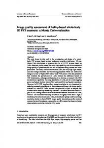
Fig. 2. Illustration of the difference between the SSIM and the proposed scheme: (a1) original image from LIVE database; (a2) JPEG image from LIVE database, , SSIM , and ; (a3) white noisy image from LIVE database, with DMOS , SSIM , and ; (b1) with DMOS and (b2) being the magnified versions of image blocks indicated by blocks in (a2) and (a3), respectively; (c1) being the SSIM map for the image blocks whose central pixels are within (b1), with the SSIM value of 0.431 for (b1); (c2) being the quality map from (5a) for the image blocks whose central pixels are within (b1), with the score from (5a) of 0.33; (c3) being the quality map from (5a) for the image blocks whose central pixels are within (b2), with the score from (5a) of 0.67 for (b2); and (c4) being the SSIM map for the image blocks whose central pixels are within (b2), with the SSIM value of 0.392 for (b2). The order of (c1)–(c4) in the figure is just arranged for easy comparison between (c1) and (c4) as well as between (c2) and (c3). Note that (c1) is almost white except for edges, and this means that the error caused by JPEG compression mainly appears in the introduced false edges; on the other hand, (c4) is with low brightness; this represents that the SSIM is quite sensitive to white noise in a smooth region (note that the image block indicated by the block in (a1) is smooth), and it is a case where SSIM overestimates the white noisy distortion.
where and are the gradient values for the central pixel of image blocks and , respectively, and is the small constant as in (2) to avoid the denominator being zero (e.g., ); is the gradient similarity between and , and its value lies in [0, 1]. The initial form of the proposed scheme in (5a) is mathematically similar to the luminance/contrast comparison term of the SSIM, and as will be demonstrated, it is more effective than that in the SSIM. An example is shown in Fig. 2. These images have been taken from the Laboratory for Image and Video Engineering (LIVE) database [23]. In this figure, (a1) is the original image, (a2) is the JPEG compressed image, and (a3) is the images with white noise; (b1) and (b2) are the amplified versions of the blocks corresponding to the same region, as highlighted in (a2) and (a3), respectively: (b1) is an edge (to be exact, due to a false edge caused by JPEG compression) block, and (b2) is a noisy block; (c1) and (c4) show the SSIM map (darker gray levels
represent larger distortion) for the image blocks whose central pixels are within (b1) and (b2), respectively; (c2) and (c3) are the quality maps from (5a) for the image blocks whose central pixels are within (b1) and (b2), respectively. As it is shown in Fig. 2, blocking in (a2) is much more annoying than white noise in (a3). This is also confirmed by the subjective differential mean opinion score (DMOS) values, which are 83.6 for (a2) and 51.4 for (a3) in LIVE database for the whole images. Note that a smaller DMOS indicates higher quality. However, Fig. 2(c1) and (c4) have similar brightness (i.e., the SSIM value) for the distortion regions, and this is not consistent with the HVS perception (i.e., the DMOS values). The quality values for (b1) and (b2) are given in the images for (c1) and (c4), respectively, and they are similar. On the contrary, as shown in (c2) and (c3), the proposed can measure the relative quality loss (mainly the quality loss around edge and that in the nonedge regions) better than the SSIM,
LIU et al.: IMAGE QUALITY ASSESSMENT BASED ON GRADIENT SIMILARITY
1503
is weak texture. As expected, the gradient values for (b1) and (b2) are different. Although both standard deviation and gradient can be used to measure the contrast, their difference is as follows. Given a group of pixel values, the standard deviation for the pixels is a constant, no matter how these pixels are positioned (i.e., independent of pixel positioning), whereas the gradient values for the same group of pixels change according to the positioning of these pixels. Note that can be rewritten as
Fig. 3. Operators for calculating the gradient value. TABLE I GRADIENT AND STANDARD DEVIATION FOR DIFFERENT IMAGE BLOCKS IN Fig. 2
with the evidence that the given value for block (b1) by (5a) is much lower than that for (b2). This is the reason why the quality scores in (5a) for (a2) and (a3) are more consistent with the DMOS values compared with the SSIM scores. The effectiveness of the proposed scheme will be further demonstrated through extensive experiments in Section V. Gradient value (same for ) is calculated as the maximum weighted average of difference for the block as [43] mean2
(6)
with , as shown in Fig. 3, where the weighting coefficient decreases as the distance from the central pixel increases, and mean is the mean value for a matrix. The Sobel or Prewitt operator is not used since the kernels are too small (3 3) to include sufficient neighboring information and only two directions (horizontal and vertical) are considered. can be interpreted either as a blockwise version (i.e., gradient similarity for image blocks and ) or a pixelwise version (i.e., the gradient similarity for the central pixels of image blocks and ). In the pixel version, we define (5b) where and are the central pixels of image blocks and , respectively. The proposed formulation for is able to measure both image contrast (the degree of signal variation) change and image structure (structure of objects in the scene) change since the gradient value (i.e., and ) is a contrast-and-structure variant feature. To illustrate this, first, consider with is a constant and , and then we have ; therefore, since , and it is shown that is a contrast variant feature. To further demonstrate that is a structure variant feature, we have shown in Table I the gradient values for (b1) and (b2) in Fig. 2. The standard deviation values (i.e., , as used in the SSIM to measure the contrast change) for the image blocks are also given for a comparison. In Table I, we can see that the values of for (b1) and (b2) are very close; however, (b1) and (b2) have very different structures, i.e., one is edge and the other
(7) with the masked gradient change defined as (8) where , and it is close to zero (when is small enough, e.g., as aforementioned); is the gradient change (i.e., ) relative to the masking gradient (note that either or is a masking signal, and here, we use the larger one, i.e., as the masking gradient) and lies in the range of [0, 1]. As it is shown in (8), when , i.e., the gradient of test image block is the same as that of reference image block ; when either or is zero (therefore, ), i.e., when either false gradient is created from an originally smooth block or an originally nonsmooth block is changed into a complete smooth one. It is revealed in (7) and (8) that, with the same amount of gradient change, the proposed is less sensitive to the case of higher masking contrast than that of lower masking contrast, and this is consistent with the contrast masking of the HVS for high masking contrast, as will be further discussed in Section III-C. B. Further Analysis for the Proposed Scheme and SSIM Consider Fig. 4 in which the -axis represents the predicted value from the scheme under consideration and the -axis represents the subjective DMOS. We show the five-parameter logistic mapping curve between the objective outputs and the subjective DMOS [the logistic mapping is to be discussed in Section V-A as (13)] as the middle curve. The upper curve denotes (here, as an example in the figure) the upper bound (i.e., with DMOS value being higher than the middle curve); the lower curve denotes the lower bound (i.e., with DMOS value being lower than the middle curve). In other words, the DMOS value of the images corresponding to the data points lying between the upper and lower curves can be “correctly” predicted
1504
IEEE TRANSACTIONS ON IMAGE PROCESSING, VOL. 21, NO. 4, APRIL 2012
Fig. 4. Predicted value from schemes under consideration ( -axis) and the subjective DMOS ( -axis; with DMOS the SSIM value. (b) DMOS versus the score from (5a).
by the IQA scheme if measurement error is allowed; the DMOS value of the remaining images cannot be “correctly” predicted from the IQA scheme. The more the data points are between the bounding curves, the better the scheme is. If a data point lies below the lower bound, it means that the visual distortion is overestimated [such as Fig. 2(c4)] since the scheme predicts a higher score (i.e., lower image quality) than the actual DMOS value; the visual distortion is underestimated for the data points lying above the upper-bound curve. Fig. 4(a) shows the plot of DMOS versus SSIM for high-distortion images (i.e., with DMOS values bigger than 50) from LIVE database, where J2K, JPG, WN, GB, and FF represent the distortion types of JPEG 2000 compression, JPEG compression, white Gaussian noise, Gaussian blur, and fast fading, respectively. In Fig. 4(a), some (more than 60 in number) data points lie outside the bounding curves; note that these data points mainly correspond to the images with WN distortion, and therefore, we have statistically demonstrated that the SSIM shows higher sensitivity to white noise, i.e., it overestimates the visual distortion with WN. It can be also observed in Fig. 4(a) that the SSIM tends to underestimate the visual distortion caused by JPEG compression. The similar plot with the data given by (5a) is shown in Fig. 4(b), and only 29 data points lie outside the bounding curves. The effect of WN is also overestimated but to a lesser extent; in addition, there is no underestimation for JPG error due to the proper emphasis on the edge information. C. Modified Gradient Similarity Here, we examine more closely on how well (7) and (8) work. With a test image block and its reference block , the gradient (or contrast) of can be regarded as the gradient of being combined with an error signal ; alternatively, the gradient of can be regarded as that of being combined with an error signal . When two visual signals combine, there is masking of one signal over the other, and a visibility threshold [12], [14], [22] can be determined for the masked contrast against the masking contrast. In general, the visibility threshold (below which the change is not noticeable to the HVS) for the masked signal
50) for LIVE database. (a) DMOS versus
increases with the masking contrast [12], [14], [22]. Masked gradient change defined in (8) is a largely reasonable choice since, when the masking signal is higher (i.e., is higher), the perceptual effect of the masked signal is lower for a same amount of (resulting in a lower ) due to higher . As discussed in Section III-A, the lower value of , the higher value for (therefore, the higher predicted quality of test block ). The only problem for the formulation with (7) and (8) is the case with both the following conditions being met: (i) causes distortion that is smaller than or close to ; and (ii) is comparable to in value. With case (i), should be 0, and therefore, should be 1, because the difference between and is not visible; however, if this situation coincides with case (ii), (8) can give a value to that is significantly bigger than 0, and this overestimates the image distortion. As a general scheme, we need to make the necessary provision for overcoming the aforementioned overestimation. To this end, in (7) is modified to satisfy the following conditions: (A) does not cause too much change to when cases (i) and (ii) do not simultaneously happen; and (B) is close to 1 for the cases with both (i) and (ii). For (A), should be comparable with (several times of) and in (7); for (B) should be much larger than (e.g., more than 20 times of) and . Note that both and lie in the range of [0, 2], and therefore, a reasonable value is for (A) and for (B). Obviously, must be adaptive to . In this paper, we have chosen as , where is a positive constant and called as a masking parameter. Typically, is around 50 and 5 for (A) and (B), respectively; hence, the choice of is between 200 and 1000 (we choose in the current stage of the work). Substituting the fine-tuned into (7), we get (9) in (9) is still in the range of [0, 1]. where To illustrate the effect of fine tuning for , Fig. 5(a) and (b) shows two simple image blocks that have gradient values of 1
LIU et al.: IMAGE QUALITY ASSESSMENT BASED ON GRADIENT SIMILARITY
Fig. 5. Simple example to demonstrate the benefit of the modification for
.
and 4, respectively; the visibility threshold for (a) is 4.7 using the method in [12]. In the figure, we can see that (a) and (b) are very similar, and this represents a case for condition (B). However, the quality score given by (5a) is 0.47 (which means that (a) and (b) are not similar). On the contrary, the score given by (9) is 0.989, which is more reasonable. IV. INTEGRATION FOR OVERALL IMAGE QUALITY In the previous section, we have proposed the gradient similarity-based scheme considering better (in comparison with the SSIM) masking effect and visibility threshold. For the parts within the dash box in the block diagram in Fig. 1, the “Masking Processing” module is used to determine the value of , and the “Contrast&Structure Comparison” module is used to get the value of as in (5a); (9) is the combination of these two modules. In (9), the gradient information of the reference and distorted images is used for evaluating the contrast and structural similarity. We also need to account for luminance similarity. In the rest of this section, we discuss how to tackle the luminance similarity and the integration of such feature with the gradient similarity measurement. A. Measurement for Luminance Distortion In addition to the contrast/structure changes, luminance changes can also cause the visible distortion although they are not as annoying as contrast/structure changes. However, (9) cannot account for the luminance change/distortion since it uses only the gradient information as the input and the gradient information is not affected by the noncontrast/structure changes. For example, the gradient information is the same if a constant value is added or subtracted from the image. Therefore, we have used the squared pixel error to measure the luminance changes in this paper after normalization by the dynamic range of the pixel values; luminance similarity can be defined as (10) where and are the pixels at position in image blocks and , respectively, and is the dynamic range of the pixel values (255 for 8-bit grayscale images); is the luminance similarity between image pixels and and also with the range of [0, 1]. B. Adaptive Distortion Integration The existing gradient-based schemes either fail to account for luminance distortion [21], [45] or use simple multiplication for
1505
the integration of the contrast–structure and luminance distortions [19], [20]. However, such integration method for luminance distortion ignores the fact that contrast–structure distortion has a higher impact on visual quality than luminance distortion, and therefore, it has degraded the overall performance of the scheme as demonstrated in [7]. A general form of integration for gradient and luminance similarities to derive the overall quality indicator for image pixel pair and can be given as (11) , , and are the abbreviated forms of , , and , respectively; is the weighting function used to adjust the relative importance of the two components. should be significantly smaller than 0.5 since, as pointed out earlier, contrast–structural distortion (i.e., ) plays a much more significant role toward final quality evaluation than the luminance distortion (i.e., ). In addition, the simultaneous existence of multiple distortion components in a neighborhood will mask the perception of each other. Since is more important as aforementioned and is more likely to be masked by the contrast–structural distortion if the contrast–structural distortion is high, weight should be adaptive with respect to (i.e., should be small when is small), i.e., we define where
(12) where is a positive weighting parameter. Since is in the range of [0, 1], also has to be significantly smaller than 0.5. We chose to be 0.1 in this paper in order to balance the following: 1) the need of accounting for luminance change for a general solution; and 2) the fact that luminance change contributes less than the structural one. We will analyze the impact of this parameter choice in Section V-E, with data from different images and distortion types, in various databases publicly available. V. OVERALL EXPERIMENTS AND RESULTS Here, we provide extensive experimental results to evaluate the overall accuracy, robustness, and efficiency with six publicly available subject-rated benchmark IQA databases. We also compare the performance of the proposed scheme [ as defined in (11)] with the state-of-the-art IQA schemes, including the SSIM [1], multiscale SSIM [2], VIF [3], VSNR [4], MAD [14], and IW-SSIM [32]; and the results for PSNR and PSNRHVS-M [5] are also included for comparison. We first introduce the databases and the evaluation criteria adopted and then present the experimental results. We will also discuss the computational complexity of the proposed scheme. A. Databases and Evaluation Criteria Six publicly available and subject-rated image databases in the IQA community are used, namely, LIVE [23], Tampere Image Database (TID) [24], [25], Toyama [26], A57 [27], IVC [28], [29], and CSIQ [14], [30]. The number of distorted images is 779 for LIVE, 1700 for TID2008, 168 for Toyama, 54 for A57, 185 for IVC, and 866 for CSIQ, and these images and
1506
IEEE TRANSACTIONS ON IMAGE PROCESSING, VOL. 21, NO. 4, APRIL 2012
Fig. 6. Scatter plots of subjective scores versus scores from the proposed scheme CSIQ.
their corresponding subjective ratings are used as the ground truths to be compared against the IQA scheme outputs. A five-parameter logistic mapping between the objective outputs and the subjective scores is employed following the Video Quality Experts Group Phase-I/II tests and validation method [33] to remove any nonlinearity due to the subjective rating process and to facilitate the comparison of the schemes in a common analysis space. The used logistic function has the following form:
on IQA databases: (a) LIVE; (b) TID; (c) Toyama; (d) A57; (e) IVC; and (f)
independent of any monotonic nonlinear mapping) and ignore the relative distance between data points. CC and RMSE are used to evaluate prediction accuracy [33]. A better objective IQA measure has a higher CC, SROCC, and KROCC, but lower RMSE values; for a perfect match between the mapped objective scores (i.e., ) and the subjective scores, CC SROCC KROCC and RMSE . More details, comparison, and discussion of these performance measures can be found in [34] and [35]. B. Overall Accuracy and Monotonicity Evaluation
(13) where are the parameters to be fitted by minimizing the sum of squared differences between the mapped values and subjective scores. The subjective scores are the mean opinion score (MOS) or DMOS between the reference and distorted images that have been provided by the IQA databases. We used four evaluation criteria to compare the performance of the IQA schemes, i.e., 1) Spearman rank-order correlation coefficient (SROCC), 2) Kendall rank-order correlation coefficient (KROCC), 3) Pearson linear correlation coefficient (CC), and 4) root-mean-squared error (RMSE), between the objective scores after nonlinear regression (i.e., ) and the subject scores. The mathematical definition of these four criteria can be found in [32]. Among these four criteria, SROCC and KROCC are employed to assess prediction monotonicity [33]. Note that these operate only on the rank of the data points (i.e., they are
Fig. 6 shows the scatter plots of the proposed IQA scheme on the six databases. The values of SROCC, KROCC, CC, and RMSE are listed in Table II, and Table III gives the 95% confidential interval (CI) of the CC values in Table II. In Table II, we can see that the proposed scheme performs consistently well across all the databases. Although the performances of the proposed scheme and multiscale SSIM and MAD are similar across databases, the proposed scheme has a clear advantage in terms of computational effort and time required (execution time will be compared in Section V-D); moreover, the proposed scheme can provide a quality map, whereas multiscale SSIM and MAD can only provide an overall quality score. With regard to IW-SSIM, it is a good IQA scheme because it basically weighs SSIM (which itself is a reasonably effective quality measure) values using weights derived via image information content [32]. Similar weighting can be employed for the proposed scheme to further improve its performance as the next step of the work since the weighting strategy is general to different schemes. Benchmarked with the
LIU et al.: IMAGE QUALITY ASSESSMENT BASED ON GRADIENT SIMILARITY
1507
TABLE II PERFORMANCE COMPARISON FOR IQA SCHEMES ON SIX DATABASES
CI
FOR
TABLE III IQA SCHEMES ON SIX DATABASES
TABLE IV AVERAGE PERFORMANCE OVER SIX DATABASES
remaining schemes, Table III shows that the proposed scheme significantly outperforms (i.e., the lower bound of CI for the proposed scheme is larger than the upper bound of CI for the scheme in comparison) on at least one database (e.g., LIVE for PSNR, VSNR, and PSNR-HVS-M; TID for SSIM and VIF). To provide an overall indication of the comparative performance of the different schemes, Table IV gives the average SROCC, KROCC, and CC results over six databases, where the average values are computed in two cases, in the same way as done in [32]. In the first case, the correlation scores are directly averaged, whereas in the second case, different weights are as-
signed to the databases depending on the number of distorted images in each database (refer to Section V-A for such numbers). In Table IV, we can see that the proposed scheme performs the best or close to the best on average no matter what kind of averaging is used and what the evaluation criterion is. C. Robustness Evaluation The robustness of the proposed scheme on different databases is also demonstrated in Table II. Note that the SSIM performs well on IVC database but not on A57 database; VIF is not good on A57 although it is the best for LIVE. Likewise, VSNR is the
1508
IEEE TRANSACTIONS ON IMAGE PROCESSING, VOL. 21, NO. 4, APRIL 2012
TABLE V SROCC COMPARISONS FOR INDIVIDUAL DISTORTION TYPES
TABLE VI EXECUTION TIME (IN SECONDS PER IMAGE) FOR DIFFERENT SCHEMES
best for A57 but is relatively poor on TID database. Overall, MAD, IW-SSIM, and the proposed scheme give more consistent and stable performances across all the six databases in comparison with the other schemes. Among the three schemes, MAD performs slightly less well on TID; IW-SSIM performs slightly less well on A57, whereas the proposed one performs slightly less well on CSIQ. To further examine the robustness of the IQA schemes, the performance on each distortion type in TID database is shown in Table V, where the two best IQA schemes have been highlighted in boldface for each distortion type. The TID database is used since it is the largest database and contains the most distortion types, which are listed in the first column of Table V. We include only the SROCC values since other performance criteria lead to similar conclusions. From the table, we can see that, for noise-contaminated images, traditional PSNR and its variant (i.e., PSNR-HVS-M) are still the best IQA schemes; the proposed scheme, the SSIM, multiscale SSIM, and IW-SSIM have similar performance. For other distortion types, the proposed scheme performs quite well (i.e., the best or the second best). Such results are expected since, for the cases where noise would not severely damage the edge or create false edge, the proposed scheme emphasizing edge information maintains the performance; when the distortion causes error both around edges and nonedges (e.g., blockwise distortion), the performance of the proposed scheme is good. It is also noted that the MAD has some difficulty to predict the quality of the images with distortions caused by mean value shift or contrast change. D. Efficiency Evaluation To compare the efficiency (i.e., computational complexity) of different schemes, we measured the average execution time required for per image (512 512 in size) in A57 database on a PC with 2.40-GHz Intel Core 2 CPU and 2 GB of RAM.
Table VI shows the required time in seconds per image, with all the codes being implemented with MATLAB. The codes for the SSIM, multiscale SSIM, VSNR, VIF, PSNR-HVS-M, MAD, and IW-SSIM are from [23], [36], [36]–[38], [46], and [47], respectively. It is shown in Table VI that the proposed scheme takes more time than the PSNR and the SSIM only, and it is faster than the multiscale SSIM since no multiscale image decomposition is involved in the proposed scheme. MAD and IW-SSIM also take much longer processing time than the proposed scheme. To be more precise, the proposed method takes only about 0.25% and 15.2% of the time taken by MAD and IW-SSIM, respectively. E. Impact of the Parameter Values The impact of the parameter values is shown with the plots of SROCC as a function of the parameter values. In the proand , where posed scheme, there are two parameters, i.e., is for the masking effect (its valuation has been determined in Section III-C) and is used to integrate contrast–structure and luminance distortions (as discussed in Section IV-B). is a reasonable choice, Fig. 7 To confirm that the chosen plots the SROCC as a function of for all the databases. As is large (e.g., can be observed, when the value of ), the value for the SROCC is nearly constant no matter what the value of is used, the difference of SROCC values for is smaller than 0.01, and this is valid for different values of to achieve the every database. Although the optimal value of highest SROCC value is different for different databases (i.e., 15 for Toyama; 40 for LIVE, IVC, and CSIQ; and 1000 for TID and A57), there are two common trends for different databases, as shown in these plots: a) SROCC drops fast when the value close to 0, and this is expected since, for a small , the of contrast masking effect for the case the masking signal is small, , the SROCC is is not properly reflected; and (b) when
LIU et al.: IMAGE QUALITY ASSESSMENT BASED ON GRADIENT SIMILARITY
Fig. 7. Plot of SROCC as a function of
1509
for (a) LIVE, (b) TID, (c) Toyama, (d) A57, (e) IVC, and (f) CSIQ databases.
Fig. 8. Plot of (a) SROCC, (b) CC, and (c) RMSE as a function of
very close to (i.e., no smaller than 97.7% of) the highest possible is used. Therefore, the value when the optimal value for is reasonable for our purpose. choice of To show the impact of for (12), we simulated various values of on TID database [25] first since it includes luminance distortion (mean shift distortion, with 25 reference images and 4 distortion levels for each reference image). In Fig. 8, we show the absolute values of the SROCC, CC, and RMSE plotted as a function of for the overall performance (i.e., the images with all the 17 distortion types) and the performance on luminance distortion (i.e., the images with mean shift distortion). We found to yield good tradeoff between performance on luthat minance distortion and for the overall cases (i.e., the SROCC is over 99% of the highest SROCC value, value for among all the possible SROCC values when different values of are used). In the figure, we can see that the overall performance decreases with the increase in (i.e., increase in the contribution of in ) since is less capable of measuring the contrast and structural distortions compared to . On the other
for the proposed integration approach and for the TID data set [25].
hand, cannot be zero since that will mean the luminance dissince tortion is completely ignored. Therefore, we use it gives good performance both for luminance distortion and for the overall case. In addition, Fig. 9 shows the SROCC values as a function of for the other databases. In the figure, we observe the following: a) for four databases, SROCC drops with the increase in ; this is expected since contrast–structural distortion is the dominant factor in IQA, and according to (11) and (12), the larger the value of , the larger the impact of the luminance distortion measurement; (b) when the value of is in the range of [0, 0.2], the values of the SROCC are nearly constant no matter what the value of is used (the difference of SROCC values for different values of is smaller than 0.01), and the values for SROCC are very close to (i.e., no smaller than 99% of) the highest possible value. Therefore, a value of in the range of [0, 0.2] is a good database-independent choice for the overall performance. ), the perHowever, if the value of is too small (i.e., formance on luminance distortion would degrade too much, as
1510
IEEE TRANSACTIONS ON IMAGE PROCESSING, VOL. 21, NO. 4, APRIL 2012
Fig. 9. Plot of SROCC as a function of
for (a) LIVE, (b) Toyama, (c) A57, (d) IVC, and (e) CSIQ databases.
TABLE VII SROCC COMPARISONS FOR EACH COMPONENT OF THE PROPOSED SCHEME
shown and discussed in Fig. 8. Therefore, the choice of is reasonable. F. Impact of Each Component of the Scheme To discuss the impact of each component in the proposed scheme toward the performance, the SROCC values for different components are given in Table VII, where is the proposed overall scheme as in (11); is the proposed gradient similarity scheme as in (9); is the initial form of the proposed gradient similarity scheme defined in (5a), without the modification in masking as in Section III-C; is the proposed scheme without gradient component [i.e., the gradient information is substituted with pixel gray level information as the input in (9)]; and and are the differences of and with , respectively. From the table, we can see that and have similar performance on each database, and this is expected since accounts for the major effect in the evaluation. The results of have shown the impact of the gradient component, and in the table, we can see that the incorporation of gradient component has improved about 0.05 in the SROCC value for LIVE database and 0.1–0.2 for the other databases; the possible reason for the smaller improvement on LIVE database is that this database contains a wider range of distortion strength and many IQA schemes can achieve good performance on it. It is also shown in that the modification for masking can achieve some performance improvement on every database; the performance improvements on LIVE and CSIQ databases are the smallest
(around 0.09) since the considered masking effect has more impact on near-threshold distortion compared with the impact on suprathreshold distortion, and the two databases have fewer images (in percentage) with near-threshold distortion; for A57 database, the performance improvement is the largest (larger than 0.3) since majority of the images in A57 database have lower distortion than the lowest quality images from most other databases. VI. CONCLUSION Since the HVS is more sensitive to the edge regions than the nonedge ones, edge information should be carefully and explicitly incorporated in designing of an IQA scheme. We have proposed a new IQA scheme based on the concept of gradient similarity to alleviate the shortcoming of the existing relevant schemes in this regard. We have demonstrated that the proposed gradient similarity measure can be used to gauge contrast and structural changes. In addition, we have made our scheme match better with the masking effect and visibility threshold. Finally, luminance similarity is devised and incorporated to form a complete quality evaluation scheme. The effectiveness of the proposed IQA scheme has been demonstrated with six public benchmark IQA databases. Compared with eight other representative and prominent IQA schemes, similar or better performance (i.e., more consistent with the human judgment) is achieved. Robustness across different databases and distortion types is also confirmed. In addition to its robustness and high accuracy, the proposed
LIU et al.: IMAGE QUALITY ASSESSMENT BASED ON GRADIENT SIMILARITY
scheme also provides the pixel error map and is relatively simple with its mathematical formulation and computational complexity, making it more practical to be used and embedded in various optimization processes in image processing tasks. ACKNOWLEDGMENT The authors would like to thank Associate Editor Prof. J. Malo and anonymous reviewers’ encouragement and constructive pieces of advise that have prompted us for new rounds of rethinking of our research, additional experiments, and clearer presentation of the technical content. REFERENCES [1] Z. Wang, A. C. Bovik, H. R. Sheikh, and E. P. Simoncelli, “Image quality assessment: From error visibility to structural similarity,” IEEE Trans. Image Process., vol. 13, no. 4, pp. 600–612, Apr. 2004. [2] Z. Wang, E. P. Simoncelli, and A. C. Bovik, “Multi-scale structural similarity for image quality assessment,” in Proc. IEEE Asilomar Conf. Signals, Syst., Comput., Pacific Grove, CA, Nov. 2003, pp. 1398–1402. [3] H. R. Sheikh and A. C. Bovik, “Image information and visual quality,” IEEE Trans. Image Process., vol. 15, no. 2, pp. 430–444, Feb. 2006. [4] D. M. Chandler and S. S. Hemami, “VSNR: A wavelet-based visual signal-to-noise-ratio for natural images,” IEEE Trans. Image Process., vol. 16, no. 9, pp. 2284–2298, Sep. 2007. [5] N. Ponomarenko, F. Silvestri, K. Egiazarian, M. Carli, J. Astola, and V. Lukin, “On between-coefficient contrast masking of DCT basis functions,” in Proc. 3rd Int. Workshop Video Process. Qual. Metrics Consum. Electron., Scottsdale, AZ, Jan. 2007. [6] A. M. Eskicioglu, A. Gusev, and A. Shnayderman, “An SVD-based gray-scale image quality measure for local and global assessment,” IEEE Trans. Image Process., vol. 15, no. 2, pp. 422–429, Feb. 2006. [7] D. Rouse and S. S. Hemami, “Understanding and simplifying the structural similarity metric,” in Proc. Int. Conf. Image Process., 2008, pp. 325–328. [8] Methodology for the Subjective Assessment of the Quality of Television Pictures Jun. 2002, Recommendation ITU-R BT.500-11. [9] S. S. Channappayya, A. C. Bovik, and R. W. Heath, “Rate bounds on SSIM index of quantized images,” IEEE Trans. Image Process., vol. 17, no. 9, pp. 1624–1639, Sep. 2008. [10] X. Gao, W. Lu, D. Tao, and X. Li, “Image quality assessment based on multiscale geometric analysis,” IEEE Trans. Image Process., vol. 18, no. 7, pp. 1409–1423, Jul. 2009. [11] Q. Ma, L. Zhang, and B. Wang, “New strategy for image and video quality assessment,” J. Electron. Imaging, vol. 19, no. 1, pp. 011019:1–011019:14, 2010. [12] A. Liu, W. Lin, M. Paul, C. Deng, and F. Zhang, “Just noticeable difference for images with decomposition model for separating edge and textured regions,” IEEE Trans. Circuits Syst. Video Technol., vol. 20, no. 11, pp. 1648–1652, Nov. 2010. [13] D. Kelly, “Motion and vision I: Stabilized images of stationary gratings,” J. Opt. Soc. Amer., vol. 69, no. 9, pp. 1266–1274, 1979. [14] E. C. Larson and D. M. Chandler, “Most apparent distortion: Full-reference image quality assessment and the role of strategy,” J. Electron. Imaging, vol. 19, no. 1, pp. 011006:1–011006:21, 2010. [15] X. Ran and N. Farvardin, “A perceptually motivated three-component image model-Part I: Description of the model,” IEEE Trans. Image Process., vol. 4, no. 4, pp. 401–415, Apr. 1995. [16] E. Ong, W. Lin, Z. Lu, S. Yao, and M. Etoh, “Visual distortion assessment with emphasis on spatially transitional regions,” IEEE Trans. Circuits Syst. Video Technol., vol. 14, no. 4, pp. 559–566, Apr. 2004. [17] Z. Wang and E. P. Simonceclli, “Translation insensitive image similarity in complex wavelet domain,” in Proc. Int. Conf. Acoust., Speech, Signal Process., 2005, pp. 573–576. [18] C. Yang, W. Gao, and L. Po, “Discrete wavelet transform-based structural similarity for image quality assessment,” in Proc. Int. Conf. Image Process., 2008, pp. 377–380. [19] G. Chen, C. Yang, and S. Xie, “Edge-based structural similarity for image quality assessment,” in Proc. Int. Conf. Acoust., Speech, Signal Process., 2006, pp. 14–19. [20] G. Chen, C. Yang, and S. Xie, “Gradient-based structural similarity for image quality assessment,” in Proc. Int. Conf. Image Process., 2006, pp. 2929–2932.
1511
[21] D. Kim, H. Han, and R. Park, “Gradient information-based image quality metric,” IEEE Trans. Consum. Electron., vol. 56, no. 2, pp. 930–936, May 2010. [22] G. Legge and J. Foley, “Contrast masking in human vision,” J. Opt. Soc. Amer., vol. 70, no. 12, pp. 1458–1471, 1980. [23] H. R. Sheikh, K. Seshadrinathan, A. K. Moorthy, Z. Wang, A. C. Bovik, and L. K. Cormack, Image and Video Quality Assessment Research at LIVE [Online]. Available: http://live.ece.utexas.edu/research/quality/ [24] N. Ponomarenko, F. Battisti, K. Egiazarian, J. Astola, and V. Lukin, “Metrics performance comparison for color image database,” in Proc. 4th Int. Workshop Video Process. Qual. Metrics Consum. Electron., Scottsdale, AZ, Jan. 2009. [25] N. Ponomarenko and K. Egiazarian, Tampere Image Database 2008 TID2008 [Online]. Available: http://www.ponomarenko.info/tid2008.htm [26] Y. Horita, K. Shibata, Y. Kawayoke, and Z. M. Parvez Sazzad, MICT Image Quality Evaluation Database [Online]. Available: http://mict. eng.u-toyama.ac.jp/ mict/index2.html [27] D. M. Chandler and S. S. Hemami, VSNR: A Wavelet-Based Visual Signal-to-Noise Ratio for Natural Images [Online]. Available: http:// foulard.ece.cornell.edu/dmc27/vsnr/vsnr.html [28] A. Ninassi, P. Le Callet, and F. Autrusseau, “Pseudo no reference image quality metric using perceptual data hiding,” in Proc. SPIE, Human Vis. Electron. Imaging, Jan. 2006, vol. 6057, p. 60570G. [29] A. Ninassi, P. Le Callet, and F. Autrusseau, Subjective Quality Assessment-IVC Database [Online]. Available: http://www2.irccyn.ecnantes.fr/ivcdb [30] E. C. Larson and D. M. Chandler, Categorical Image Quality (CSIQ) Database [Online]. Available: http://vision.okstate.edu/csiq [31] Y. H. Huang, T. S. Ou, P. Y. Su, and H. H. Chen, “Perceptual rate-distortion optimization using structural similarity index as quality metric,” IEEE Trans. Circuits Syst. Video Technol., vol. 20, no. 11, pp. 1614–1624, Jul. 2010. [32] Z. Wang and Q. Li, “Information content weighting for perceptual image quality assessment,” IEEE Trans. Image Process., vol. 20, no. 5, pp. 1185–1198, May 2011. [33] Video Quality Expert Group (VQEG), Final Report From the Video Quality Experts Group on the Validation of Objective Models of Video Quality Assessment II [Online]. Available: http://www.vqeg.org/ 2003 [34] H. R. Sheikh, M. F. Sabir, and A. C. Bovik, “A statistical evaluation of recent full reference image quality assessment algorithms,” IEEE Trans. Image Process., vol. 15, no. 11, pp. 3440–3451, Nov. 2006. [35] A. K. Moorthy and A. C. Bovik, “Visual importance pooling for image quality assessment,” IEEE J. Sel. Topics Signal Process., vol. 3, no. 2, pp. 193–201, Apr. 2009. [36] Z. Wang, A. Bovik, H. Sheikh, and E. Simoncelli, The SSIM Index for Image Quality Assessment [Online]. Available: http://ece.uwaterloo.ca/~z70wang/research/ssim/ [37] MeTriX MuX Visual Quality Assessment Package [Online]. Available: http://foulard.ece.cornell.edu/gaubatz/metrix_mux/ [38] PSNR-HVS-M Download Page [Online]. Available: http://www.ponomarenko.info/psnrhvsm.htm [39] D. M. Rouse and S. S. Hemami, “Analyzing the role of visual structure in the recognition of natural image content with multi-scale SSIM,” in Proc. Western New York Image Process. Workshop, Rochester, NY, Oct. 2007. [40] W. Lin, L. Dong, and P. Xue, “Visual distortion gauge based on discrimination of noticeable contrast changes,” IEEE Trans. Circuits Syst. Video Technol., vol. 15, no. 7, pp. 900–909, Jul. 2005. [41] Z. Wang, A. C. Bovik, and L. Lu, “Why is image quality assessment so difficult,” in Proc. Int. Conf. Acoust., Speech, Signal Process., May 2002, pp. IV-3313–IV-3316. [42] Z. Wang and A. C. Bovik, “A universal image quality index,” IEEE Signal Process. Lett., vol. 9, no. 3, pp. 81–84, Mar. 2002. [43] X. Yang, W. Lin, Z. Lu, E. Ong, and S. Yao, “Just noticeable distortion model and its applications in video coding,” Signal Process., Image Commun., vol. 20, no. 7, pp. 662–680, Aug. 2005. [44] W. Lin and C.-C. Jay Kuo, “Perceptual visual quality metrics: A survey,” J. Visual Commun. Image Representation, vol. 22, no. 4, pp. 297–312, May 2011. [45] G. Cheng, J. Huang, C. Zhu, Z. Liu, and L. Cheng, “Perceptual image quality assessment using a geometric structural distortion model,” in Proc. Int. Conf. Image Process., 2010, pp. 325–328. [46] E. Larson and D. Chandler, Full-Reference Image Quality Assessment and the Role of Strategy: The Most Apparent Distortion [Online]. Available: http://vision.okstate.edu/mad/ [47] Z. Wang, IW-SSIM: Information Content Weighted Structural Similarity Index for Image Quality Assessment [Online]. Available: https:// ece.uwaterloo.ca/~z70wang/research/iwssim/
1512
IEEE TRANSACTIONS ON IMAGE PROCESSING, VOL. 21, NO. 4, APRIL 2012
Anmin Liu received the B.Sc. degree in information science and electronic engineering from Zhejiang University, Hangzhou, China, in 2007. He is currently working toward the Ph.D. degree in the School of Computer Engineering, Nanyang Technological University, Singapore. His research interests include image/video coding, quality evaluation, and perceptual modeling and processing.
Weisi Lin (M’92–SM’98) received the B.Sc. degree in electronics and the M.Sc. degree in digital signal processing from Zhongshan University, Guangzhou, China, in 1982 and 1985, respectively, and the Ph.D. degree in computer vision from King’s College London, London, U.K., in 1992. He taught and conducted research at Zhongshan University; Shantou University, China; Bath University, U.K.; National University of Singapore, Singapore; Institute of Microelectronics, Singapore; and Institute for Infocomm Research, Singapore. He has been the Project Leader of 13 major successfully delivered projects in digital multimedia technology development. He also served as the Laboratory Head of Visual Processing Laboratory and the Acting Department Manager of Media Processing Department of the Institute for Infocomm Research . He is currently an Associate Professor with the School of Computer Engineering, Nanyang Technological University, Singapore. He edited one book, authored one book and five book chapters, and has published over 190 refereed papers in international journals and conferences. He believes that good theory is practical,
and so, he has kept a balance of academic research and industrial deployment throughout his working life. His areas of expertise include image processing, perceptual modeling, video compression, multimedia communication, and computer vision. Dr. Lin is a Fellow of the Institution of Engineering Technology and an Honorary Fellow of Singapore Institute of Engineering Technologists. He is also a Chartered Engineer (U.K.). He organized special sessions in IEEE ICME06, IEEE IMAP07, IEEE ISCAS10, PCM09, SPIE VCIP10, APSIPA11, and MobiMedia11. He gave invited/keynote/panelist talks in VPQM06, IEEE ICCCN07, SPIE VCIP10, and IEEE MMTC QoEIG (2011), as well as tutorials in PCM07, PCM09, IEEE ISCAS08, IEEE ICME09, APSIPA10, and IEEE ICIP10 . He currently serves in the editorial boards of IEEE TRANSACTIONS ON MULTIMEDIA, IEEE Signal Processing Letters, and Journal of Visual Communication and Image Representation, as well as in four IEEE Technical committees. He cochairs the IEEE Multimedia Communications Technical Committee Special Interest Group on Quality of Experience. He has been on the Technical Program committees and/or Organizing committees of a number of international conferences.
Manish Narwaria received the B.Tech. degree in electronics and communication engineering from Amrita Vishwa Vidyapeetham University, Coimbatore, India, in 2008. He is currently working toward the Ph.D. degree in the School of Computer Engineering, Nanyang Technological University, Singapore. His research interests include image/video and speech quality assessment, pattern recognition, and machine learning.