Immersed Finite Element Particle-In-Cell Simulations of ... - VTechWorks

Immersed Finite Element Particle-In-Cell Simulations of Ion Propulsion

Raed I. Kafafy

Dissertation submitted to the Faculty of the Virginia Polytechnic Institute and State University in partial fulfillment of the requirements for the degree of

Doctor of Philosophy in Aerospace Engineering

Joseph Wang, Chair Slimane Adjred Tao Lin Calvin Ribbens Joseph Schetz

September 1, 2005 Blacksburg, Virginia

Keywords: Electric Propulsion, Ion Thruster, Finite Element, Particle-in-Cell Copyright 2005, Raed I. Kafafy

Immersed Finite Element Particle-In-Cell Simulations of Ion Propulsion

Raed I. Kafafy

(ABSTRACT)

A new particle-in-cell algorithm was developed for plasma simulations involving complex boundary conditions. The new algorithm is based on the three-dimensional immersed finite element method which is developed in this dissertation, and a modified legacy particle-in-cell code. The model also applies a new meshing technique that separates the field solution mesh from the particle pushing mesh in order to increase the computational efficiency of the model. The new simulation model is used in two applications of great importance to the development of ion propulsion technology: the ion optics performance and the interaction between spacecraft and the ion thruster. The first application is ion optics simulations. Simulations are performed to investigate ion optics plasma flow for a whole subscale NEXT ion optics. The operating conditions modeled cover the entire cross-over to perveance limit range. The results of the ion optics simulations demonstrated good agreement with the available experimental data. The second application is ion thruster plume simulations. Simulations are performed to investigate ion thruster plume - spacecraft interactions for the Dawn spacecraft. Plume induced contaminations on the solar array are studied for a variety of ion thruster configurations including multiple thruster firings.

Dedication To my Parents ...

iii

Acknowledgments Praise is due to Allah, the Cherisher and Sustainer of the Worlds. First, I would like to thank my advisor, Prof. Joseph Wang from the Aerospace and Ocean Engineering Department of Virginia Tech, for all his teaching, guidance and support throughout this dissertation. His insight and comprehensive knowledge of Plasma Physics and the art of Particle Simulation provided me a great opportunity of learning. I would like also to thank Prof. Tao Lin from the Department of Mathematics of Virginia Tech, for his invaluable advices and patience to teach me the art of Finite Element Analysis. I am also grateful to the other members of my committee: Prof. Joseph Schetz from the Aerospace and Ocean Engineering Department, Prof. Slimane Adjerid from the Department of Mathematics, and Prof. Calvin Ribbens from the Department of Computer Science for their valuable advices and serving on my dissertation committee. Furthermore, I would like to acknowledge my colleagues at the Computational Advanced Propulsion Laboratory (CAPLab) of Virginia Tech for their valuable assistance and discussions. Finally, I would like to thank my wife and daughter for their patience, understanding, and inspiration throughout this dissertation. This work was supported by assistantships from the Department of Aerospace and Ocean Engineering at Virginia Tech and by the Air Force Research Laboratory (AFRL) through a grant from ERC, Inc.

iv

Contents 1 Introduction

1

1.1

Introduction . . . . . . . . . . . . . . . . . . . . . . . . . . . . . . . .

1

1.2

Background . . . . . . . . . . . . . . . . . . . . . . . . . . . . . . . .

1

1.2.1

Electric Propulsion . . . . . . . . . . . . . . . . . . . . . . . .

2

1.2.2

Ion Propulsion . . . . . . . . . . . . . . . . . . . . . . . . . .

3

1.2.3

Ion Thruster Lifetime and Failure Modes . . . . . . . . . . . .

7

1.2.4

Spacecraft-Ion Thruster Interaction and Integration Problems

8

1.3

Modeling Ion Propulsion . . . . . . . . . . . . . . . . . . . . . . . . .

9

1.4

Motivation . . . . . . . . . . . . . . . . . . . . . . . . . . . . . . . . .

10

1.5

Research Objectives . . . . . . . . . . . . . . . . . . . . . . . . . . . .

11

1.6

Organization of the Dissertation . . . . . . . . . . . . . . . . . . . . .

11

2 Literature Review

13

2.1

Introduction . . . . . . . . . . . . . . . . . . . . . . . . . . . . . . . .

2.2

Previous Work On Ion Optics Simulation – Review of the Last Decade 14

2.3

Previous Work On Spacecraft–Ion Thruster Plume Interaction – Review of the Last Decade . . . . . . . . . . . . . . . . . . . . . . . . .

17

Review On Methods To Solve A Field Problem With Complex Boundaries . . . . . . . . . . . . . . . . . . . . . . . . . . . . . . . . . . . .

21

2.4

v

13

2.4.1

Body-Fitting-Grid Methods . . . . . . . . . . . . . . . . . . .

22

2.4.2

Cartesian-Grid Methods Based On Finite Difference Discretization . . . . . . . . . . . . . . . . . . . . . . . . . . . . . . . .

23

2.4.3 2.5

Cartesian-Grid Methods Based On Finite Element Discretization 25

Contribution . . . . . . . . . . . . . . . . . . . . . . . . . . . . . . . .

3 A Three-Dimensional Immersed Finite Element Method

27 29

3.1

Introduction . . . . . . . . . . . . . . . . . . . . . . . . . . . . . . . .

29

3.2

The Interface Boundary Value Problem . . . . . . . . . . . . . . . . .

29

3.3

Weak Formulation Of The Field Problem . . . . . . . . . . . . . . . .

31

3.4

A Three–Dimensional IFE Space . . . . . . . . . . . . . . . . . . . .

32

3.4.1

Intersection Topology . . . . . . . . . . . . . . . . . . . . . . .

34

3.4.2

Special Intersection Topology . . . . . . . . . . . . . . . . . .

34

3.4.3

Linear Local Nodal FE Basis Functions . . . . . . . . . . . . .

36

3.4.4

Linear Local Nodal IFE Basis Functions . . . . . . . . . . . .

36

3.4.5

Existence and Uniqueness . . . . . . . . . . . . . . . . . . . .

43

3.4.6

Partition of Unity and Consistency with Classical FEM . . . .

45

Numerical Experiments . . . . . . . . . . . . . . . . . . . . . . . . . .

47

3.5.1

An Interface Problem With a Spherical Interface . . . . . . . .

48

3.5.2

An Interface Problem With a Hemispherical Interface . . . . .

50

3.5.3

Numerical Error Analysis . . . . . . . . . . . . . . . . . . . .

53

3.5

4 Three-Dimensional IFE Field Solver

58

4.1

Introduction . . . . . . . . . . . . . . . . . . . . . . . . . . . . . . . .

58

4.2

Mesh Generation . . . . . . . . . . . . . . . . . . . . . . . . . . . . .

58

4.3

Mesh-Object Intersection . . . . . . . . . . . . . . . . . . . . . . . . .

59

4.3.1

59

Intersection Topology Classification . . . . . . . . . . . . . . . vi

4.4

4.5

4.6

4.7

Assembly of the IFE System . . . . . . . . . . . . . . . . . . . . . . .

61

4.4.1

Local Assembler . . . . . . . . . . . . . . . . . . . . . . . . . .

61

4.4.2

Global Assembler . . . . . . . . . . . . . . . . . . . . . . . . .

62

4.4.3

Integration Rules . . . . . . . . . . . . . . . . . . . . . . . . .

62

4.4.4

Sparse Storage of the System Matrix . . . . . . . . . . . . . .

64

Solution of the Nonlinear Field Problem . . . . . . . . . . . . . . . .

67

4.5.1

Gauss-Seidel Iteration . . . . . . . . . . . . . . . . . . . . . .

67

4.5.2

Newton-Raphson Iteration . . . . . . . . . . . . . . . . . . . .

68

Solution of the Sparse Linear/Linearized System . . . . . . . . . . . .

69

4.6.1

Preconditioned-Conjugate Gradient (PCCG) Solver . . . . . .

69

4.6.2

Preconditioners . . . . . . . . . . . . . . . . . . . . . . . . . .

69

Hardwiring The IFE Field Solver . . . . . . . . . . . . . . . . . . . .

71

5 The Hybrid-Grid IFE-PIC Model

73

5.1

Introduction . . . . . . . . . . . . . . . . . . . . . . . . . . . . . . . .

73

5.2

Theory . . . . . . . . . . . . . . . . . . . . . . . . . . . . . . . . . . .

74

5.2.1

Plasma . . . . . . . . . . . . . . . . . . . . . . . . . . . . . . .

74

5.2.2

Debye Shielding and Plasma Sheath . . . . . . . . . . . . . . .

75

The Particle–In–Cell Method . . . . . . . . . . . . . . . . . . . . . .

75

5.3.1

Particle Push . . . . . . . . . . . . . . . . . . . . . . . . . . .

76

5.3.2

Charge Deposit . . . . . . . . . . . . . . . . . . . . . . . . . .

77

5.3.3

Field Solve . . . . . . . . . . . . . . . . . . . . . . . . . . . . .

78

5.3.4

Force Weighting . . . . . . . . . . . . . . . . . . . . . . . . . .

79

Particles Initial and Boundary Conditions . . . . . . . . . . . . . . .

79

5.4.1

Particles Loading . . . . . . . . . . . . . . . . . . . . . . . . .

79

5.4.2

Particles Injection . . . . . . . . . . . . . . . . . . . . . . . . .

80

5.3

5.4

vii

5.4.3

Particles Boundary Conditions . . . . . . . . . . . . . . . . . .

80

5.5

The IFE–PIC Model . . . . . . . . . . . . . . . . . . . . . . . . . . .

82

5.6

The Concept of Hybrid–Grid . . . . . . . . . . . . . . . . . . . . . . .

83

5.6.1

IFE Mesh Stretching . . . . . . . . . . . . . . . . . . . . . . .

83

5.6.2

IFE Mesh Stretching Rule . . . . . . . . . . . . . . . . . . . .

84

HG–IFE–PIC Interpolation Procedure . . . . . . . . . . . . . . . . .

85

5.7.1

Particle-PIC Deposition . . . . . . . . . . . . . . . . . . . . .

85

5.7.2

PIC-IFE Mesh Interpolation . . . . . . . . . . . . . . . . . . .

86

5.7.3

IFE-PIC Mesh Interpolation . . . . . . . . . . . . . . . . . . .

87

Numerical Experiments . . . . . . . . . . . . . . . . . . . . . . . . . .

87

5.8.1

Single Particle Motion . . . . . . . . . . . . . . . . . . . . . .

87

5.8.2

Plasma Flow Through Ion Optics . . . . . . . . . . . . . . . .

88

5.7

5.8

6 Ion Optics Simulations

91

6.1

Introduction . . . . . . . . . . . . . . . . . . . . . . . . . . . . . . . .

91

6.2

Physical and Mathematical Modeling of Ion Optics . . . . . . . . . .

92

6.2.1

Upstream Discharge Chamber Plasma . . . . . . . . . . . . .

92

6.2.2

Ion Optics Beam Extraction . . . . . . . . . . . . . . . . . . .

93

6.2.3

Downstream Neutralization Plasma . . . . . . . . . . . . . . .

93

6.2.4

Dynamics of Beam Ions . . . . . . . . . . . . . . . . . . . . .

93

6.2.5

Electrostatic Field . . . . . . . . . . . . . . . . . . . . . . . .

94

6.2.6

Beam Current Extraction . . . . . . . . . . . . . . . . . . . .

94

6.2.7

Impingement Current Limits . . . . . . . . . . . . . . . . . . .

96

6.2.8

Electron Backstreaming . . . . . . . . . . . . . . . . . . . . .

97

6.3

Normalization . . . . . . . . . . . . . . . . . . . . . . . . . . . . . . .

98

6.4

Simulation Model . . . . . . . . . . . . . . . . . . . . . . . . . . . . .

99

viii

6.4.1

Simulation Domain . . . . . . . . . . . . . . . . . . . . . . . .

99

6.4.2

Simulation Algorithm . . . . . . . . . . . . . . . . . . . . . . . 100

6.4.3

Streamline PIC Simulation . . . . . . . . . . . . . . . . . . . . 103

6.5

NEXT Ion Optics . . . . . . . . . . . . . . . . . . . . . . . . . . . . . 105

6.6

Simulation Domain Layout . . . . . . . . . . . . . . . . . . . . . . . . 106

6.7

Standard HG-IFE-PIC Simulation . . . . . . . . . . . . . . . . . . . . 107

6.8

6.9

6.7.1

Simulation Setup . . . . . . . . . . . . . . . . . . . . . . . . . 108

6.7.2

Computational Performance . . . . . . . . . . . . . . . . . . . 109

6.7.3

Beamlet Behavior . . . . . . . . . . . . . . . . . . . . . . . . . 110

6.7.4

Impingement Current . . . . . . . . . . . . . . . . . . . . . . . 113

Streamline HG-IFE-PIC Simulation: Two-Quarter Aperture . . . . . 114 6.8.1


6.8.2


6.8.3

Beamlet Behavior . . . . . . . . . . . . . . . . . . . . . . . . . 115

6.8.4

Impingement Current Limits . . . . . . . . . . . . . . . . . . . 118

6.8.5

Electron Backstreaming Limit . . . . . . . . . . . . . . . . . . 118

Streamline HG-IFE-PIC Simulation: Whole Subscale Gridlet . . . . . 120 6.9.1


6.9.2


6.9.3

Beamlet Plasma Flow

6.9.4

Impingement Current Limits . . . . . . . . . . . . . . . . . . . 125

6.9.5

Electron Backstreaming Limit . . . . . . . . . . . . . . . . . . 129

. . . . . . . . . . . . . . . . . . . . . . 123

6.10 Summary and Conclusion . . . . . . . . . . . . . . . . . . . . . . . . 130 7 Ion Thruster Plume Simulations 7.1

133

Introduction . . . . . . . . . . . . . . . . . . . . . . . . . . . . . . . . 133

ix

7.2

7.3

Spacecraft Contamination . . . . . . . . . . . . . . . . . . . . . . . . 134 7.2.1

Modeling of Contamination . . . . . . . . . . . . . . . . . . . 134

7.2.2

Measuring Molecular Film Thickness . . . . . . . . . . . . . . 136

Modelling of Ion Thruster Plume . . . . . . . . . . . . . . . . . . . . 136 7.3.1

Ion Beam . . . . . . . . . . . . . . . . . . . . . . . . . . . . . 137

7.3.2

Neutral Propellant Plume . . . . . . . . . . . . . . . . . . . . 139

7.3.3

Charge-Exchange Ions . . . . . . . . . . . . . . . . . . . . . . 140

7.3.4

Non-Propellant Efflux . . . . . . . . . . . . . . . . . . . . . . 140

7.3.5

Electrons . . . . . . . . . . . . . . . . . . . . . . . . . . . . . 141

7.3.6

Electrostatic Field . . . . . . . . . . . . . . . . . . . . . . . . 142

7.4

Normalization . . . . . . . . . . . . . . . . . . . . . . . . . . . . . . . 142

7.5

Simulation Model . . . . . . . . . . . . . . . . . . . . . . . . . . . . . 143

7.6

7.5.1

Simulation Domain . . . . . . . . . . . . . . . . . . . . . . . . 143

7.5.2

Simulation Algorithm . . . . . . . . . . . . . . . . . . . . . . . 143

7.5.3

Deposit Calculation . . . . . . . . . . . . . . . . . . . . . . . . 145

Dawn Spacecraft . . . . . . . . . . . . . . . . . . . . . . . . . . . . . 146 7.6.1

Spacecraft . . . . . . . . . . . . . . . . . . . . . . . . . . . . . 146

7.6.2

Ion Thruster . . . . . . . . . . . . . . . . . . . . . . . . . . . . 147

7.7

Spacecraft Model . . . . . . . . . . . . . . . . . . . . . . . . . . . . . 148

7.8

Simulation Domain . . . . . . . . . . . . . . . . . . . . . . . . . . . . 149

7.9

Simulation Setup . . . . . . . . . . . . . . . . . . . . . . . . . . . . . 150

7.10 Results: CASE 0 . . . . . . . . . . . . . . . . . . . . . . . . . . . . . 151 7.10.1 Plasma Diagnosis . . . . . . . . . . . . . . . . . . . . . . . . . 152 7.10.2 Deposition Diagnosis . . . . . . . . . . . . . . . . . . . . . . . 153 7.11 Results: CASE 1 . . . . . . . . . . . . . . . . . . . . . . . . . . . . . 153 7.11.1 Plasma Diagnosis . . . . . . . . . . . . . . . . . . . . . . . . . 156 x

7.11.2 Deposition Diagnosis . . . . . . . . . . . . . . . . . . . . . . . 159 7.12 Results: CASE 2 . . . . . . . . . . . . . . . . . . . . . . . . . . . . . 162 7.12.1 Plasma Diagnosis . . . . . . . . . . . . . . . . . . . . . . . . . 164 7.12.2 Deposition Diagnosis . . . . . . . . . . . . . . . . . . . . . . . 165 7.13 Summary and Conclusion . . . . . . . . . . . . . . . . . . . . . . . . 167 8 Conclusions

170

8.1

Introduction . . . . . . . . . . . . . . . . . . . . . . . . . . . . . . . . 170

8.2

Summary of Research . . . . . . . . . . . . . . . . . . . . . . . . . . . 170

8.3

Contributions to Finite Element Analysis . . . . . . . . . . . . . . . . 171

8.4

Contributions to Plasma Simulation . . . . . . . . . . . . . . . . . . . 171

8.5

Contributions to Ion Optics Modeling . . . . . . . . . . . . . . . . . . 172

8.6

Contributions to Spacecraft-Ion Thruster Interaction Modeling . . . . 173

8.7

Recommended Future Work . . . . . . . . . . . . . . . . . . . . . . . 173

xi

List of Figures 1.1

NSTAR ion thruster. . . . . . . . . . . . . . . . . . . . . . . . . . . .

4

1.2

A schematic of an ion thruster. . . . . . . . . . . . . . . . . . . . . .

6

3.1

Solution domain of the interface BVP. . . . . . . . . . . . . . . . . .

30

3.2

Partitioning of a Cartesian IFE cell. . . . . . . . . . . . . . . . . . . .

32

3.3

The five tetrahedra comprising a Cartesian cell. . . . . . . . . . . . .

33

3.4

Intersection topologies of tetrahedral elements. . . . . . . . . . . . . .

35

3.5

An odd intersection topology. . . . . . . . . . . . . . . . . . . . . . .

35

3.6

Two cases of possible three-edge cut in the reference element Tˆ. . . .

38

3.7

One of the three possible four-edge cut elements in the reference element Tˆ. . . . . . . . . . . . . . . . . . . . . . . . . . . . . . . . . . .

41

3.8

Geometry of the spherical interface problem. . . . . . . . . . . . . . .

49

3.9

Interpolation and solution errors of a spherical-interface problem. . .

52

3.10 Geometry of the hemispherical interface problem. . . . . . . . . . . .

53

3.11 Interpolation and solution errors of a hemispherical-interface problem.

56

4.1

Special situations of three-edge cut tetrahedron. . . . . . . . . . . . .

60

4.2

Partitioning of typical interface tetrahedra into sub-tetrahedra. . . . .

64

4.3

Sub-tetrahedra in a three-edge cut element.

. . . . . . . . . . . . . .

65

4.4

Sub-tetrahedra in a four-edge cut element. . . . . . . . . . . . . . . .

66

xii

4.5

Preconditioned conjugate gradient algorithm. . . . . . . . . . . . . . .

70

4.6

Incomplete Cholesky decomposition preconditioner. . . . . . . . . . .

71

5.1

Illustration of the leap-frog scheme. . . . . . . . . . . . . . . . . . . .

77

5.2

Deposition of particle charge in a two-dimensional simulation domain.

78

5.3

Reflection particle boundary conditions. . . . . . . . . . . . . . . . .

81

5.4

Interpolation procedure for a collocated IFE-PIC mesh. . . . . . . . .

82

5.5

IFE–cell stretching. . . . . . . . . . . . . . . . . . . . . . . . . . . . .

83

5.6

Mesh stretching for various stretching parameters. . . . . . . . . . . .

85

5.7

Interpolation procedure for a hybrid-grid IFE-PIC. The PIC mesh is shown in light grey and the IFE mesh in dark grey. . . . . . . . . . .

86

5.8

Simulation domain of the single particle motion experiment. . . . . .

88

5.9

Effect of stretching parameter on the trajectory of a single charged particle. . . . . . . . . . . . . . . . . . . . . . . . . . . . . . . . . . .

89

5.10 Simulation domain of the ion optics plasma flow experiment. . . . . .

90

5.11 Effect of stretching parameter on ion optics potential solution. . . . .

90

6.1

Grid system parameters. . . . . . . . . . . . . . . . . . . . . . . . . .

95

6.2

Focusing of the ion beamlet. . . . . . . . . . . . . . . . . . . . . . . .

97

6.3

Two-quarter aperture simulation domain. . . . . . . . . . . . . . . . . 107

6.4

Whole ion optics simulation domain. . . . . . . . . . . . . . . . . . . 108

6.5

IFE and PIC meshes used in the simulation of NEXT ion optics at n0 = 1.0 × 1017 m−3 . . . . . . . . . . . . . . . . . . . . . . . . . . . . . 110

6.6

Beamlet plasma potential and ion density. Ion density is normalized by n0 = 1.0 × 1017 m−3 . Potential contour lines are shown for the values from −210 V to 1790 V with a step of 200 V. The 1780 V, 1795 V and zero potential contour lines are also shown. . . . . . . . . . . . 111

xiii

6.7

Beamlet plasma potential. Potential contour lines are shown for the values from −210 V to 1790 V with a step of 200 V. The 1780 V, 1795 V and zero potential contour lines are also shown. Potential is normalized by Te0 =5 eV. . . . . . . . . . . . . . . . . . . . . . . . . 112

6.8

Convergence history of the streamline HG-IFE-PIC simulation at n0 = 0.05 × 1017 m−3 . . . . . . . . . . . . . . . . . . . . . . . . . . . . . . . 115

6.9

Beamlet plasma potential and ion density. Ion density is normalized by n0 = 1.0 × 1017 m−3 . Potential contour lines are shown for the values from −210 V to 1790 V with a step of 200 V. The 1780 V, 1795 V and zero potential contour lines are also shown. . . . . . . . . . . . 116

6.10 Beamlet plasma potential. Potential contour lines are shown for the values from −210 V to 1790 V with a step of 200 V. The 1780 V, 1795 V and zero potential contour lines are also shown.Potential is normalized by Te0 =5 eV. . . . . . . . . . . . . . . . . . . . . . . . . 117 6.11 Impingement current limits for the two-quarter apertures (single aperture) model. . . . . . . . . . . . . . . . . . . . . . . . . . . . . . . . . 119 6.12 Cross-over limit data collected at CSU for several screen apertures and total voltages. . . . . . . . . . . . . . . . . . . . . . . . . . . . . 120 6.13 Potential profile along aperture centerline. . . . . . . . . . . . . . . . 121 6.14 Aperture electron backstreaming. . . . . . . . . . . . . . . . . . . . . 121 6.15 IFE and PIC meshes used in the simulation of NEXT ion optics at n0 = 1.0 × 1017 m−3 . . . . . . . . . . . . . . . . . . . . . . . . . . . . . 123 6.16 Comparison of CPU time for different ion optics models. . . . . . . . 124 6.17 Beamlet plasma normalized potential and ion density at the nominal operating condition. The ion density is normalized by the nominal upstream plasma density, n0 = 1.0 × 1017 m−3 , and the potential is normalized by Te0 = 5 eV. . . . . . . . . . . . . . . . . . . . . . . . . 125 6.18 Beamlet plasma normalized potential and ion density at cross-over. The ion density is normalized by the nominal upstream plasma density, n0 = 1.0 × 1017 m−3 , and the potential is normalized by Te0 = 5 eV. . 126

xiv

6.19 Beamlet plasma normalized potential and ion density at perveance. The ion density is normalized by the nominal upstream plasma density, n0 = 1.0 × 1017 m−3 , and the potential is normalized by Te0 = 5 eV. . 127 6.20 Impingement current curve for the whole gridlet (seven apertures) model as compared with the two-quarter aperture (single aperture) model. . . . . . . . . . . . . . . . . . . . . . . . . . . . . . . . . . . . 128 6.21 Impingement current limits. . . . . . . . . . . . . . . . . . . . . . . . 129 6.22 Potential profile along aperture centerlines. . . . . . . . . . . . . . . . 130 6.23 Aperture electron backstreaming. . . . . . . . . . . . . . . . . . . . . 131 7.1

Geometry of beam profile. . . . . . . . . . . . . . . . . . . . . . . . . 138

7.2

Geometry of neutral plume profile. . . . . . . . . . . . . . . . . . . . 139

7.3

Dawn spacecraft layout. . . . . . . . . . . . . . . . . . . . . . . . . . 147

7.4

Geometry of the studied Dawn thruster configurations. . . . . . . . . 149

7.5

A 3D view of the IFE mesh. The mesh is cut away to illustrate relative spacecraft position. . . . . . . . . . . . . . . . . . . . . . . . . . . . . 150

7.6

History of number of particles for Xe+ CEX ions simulation for CASE 0A. The simulation time is given in units of time steps. . . . . . . . . 151

7.7

Plasma properties for CASE 0A. Potential is normalized by 5 eV and ion charge density is normalized by 7.61 × 1010 m−3 . . . . . . . . . . . 152

7.8

Xe+ CEX ion trajectories for CASE 0A. . . . . . . . . . . . . . . . . 153

7.9

Deposition flux of Mo atoms for CASE 0A. . . . . . . . . . . . . . . . 154

7.10 Firing options of CASE 1. . . . . . . . . . . . . . . . . . . . . . . . . 154 7.11 History of number of particles for Xe+ CEX ions simulation for CASE 1 with all possible firing options. The simulation time is given in units of time steps. . . . . . . . . . . . . . . . . . . . . . . . . . . . . . . . 155 7.12 Plasma properties for CASE 1A. Potential is normalized by 5 eV and ion charge density is normalized by 7.61 × 1010 m−3 . . . . . . . . . . . 156 7.13 Xe+ CEX ion trajectories for CASE 1A. . . . . . . . . . . . . . . . . 157

xv

7.14 Plasma properties for CASE 1B. Potential is normalized by 5 eV and ion charge density is normalized by 7.61 × 1010 m−3 . . . . . . . . . . . 158 7.15 Xe+ CEX ion trajectories for CASE 1B. . . . . . . . . . . . . . . . . 158 7.16 Plasma properties for CASE 1C. Potential is normalized by 5 eV and ion charge density is normalized by 7.61 × 1010 m−3 . . . . . . . . . . . 159 7.17 Xe+ CEX ion trajectories for CASE 1C. . . . . . . . . . . . . . . . . 160 7.18 Deposition flux of Mo atoms for CASE 1A. . . . . . . . . . . . . . . . 160 7.19 Deposition flux of Mo atoms for CASE 1B. . . . . . . . . . . . . . . . 161 7.20 Deposition flux of Mo atoms for CASE 1C. . . . . . . . . . . . . . . . 162 7.21 Firing options of CASE 2. . . . . . . . . . . . . . . . . . . . . . . . . 163 7.22 History of number of particles for Xe+ CEX ions simulation for CASE 2 with all possible firing options. The simulation time is given in units of time steps. . . . . . . . . . . . . . . . . . . . . . . . . . . . . . . . 163 7.23 Plasma properties for CASE 2A. Potential is normalized by 5 eV and ion charge density is normalized by 7.61 × 1010 m−3 . . . . . . . . . . . 164 7.24 Xe+ CEX ion trajectories for CASE 2A. . . . . . . . . . . . . . . . . 165 7.25 Plasma properties for CASE 2B. Potential is normalized by 5 eV and ion charge density is normalized by 7.61 × 1010 m−3 . . . . . . . . . . . 166 7.26 Xe+ CEX ion trajectories for CASE 2B. . . . . . . . . . . . . . . . . 166 7.27 Deposition flux of Mo atoms for CASE 2A. . . . . . . . . . . . . . . . 167 7.28 Deposition flux of Mo atoms for CASE 2B. . . . . . . . . . . . . . . . 168

xvi

List of Tables 1.1

Specific impulse of current flight propulsion systems. . . . . . . . . .

3

3.1

L2 and H 1 interpolation errors of IFE functions generated with partitions of decreasing size h and β + /β − = 10. . . . . . . . . . . . . . .

50

L2 and H 1 interpolation errors of IFE functions generated with partitions of decreasing size h and β + /β − = 10, 000. . . . . . . . . . . . .

50

L∞ , L2 and H 1 errors of the IFE solutions generated with partitions of decreasing size h and β + /β − = 10. . . . . . . . . . . . . . . . . . .

51

L∞ , L2 and H 1 errors of the IFE solutions generated with partitions of decreasing size h and β + /β − = 10, 000. . . . . . . . . . . . . . . . .

51

L2 and H 1 interpolation errors of IFE functions generated with partitions of decreasing size h and β + /β − = 10. . . . . . . . . . . . . . .

54

L2 and H 1 interpolation errors of IFE functions generated with partitions of decreasing size h and β + /β − = 10, 000. . . . . . . . . . . . .

54

L∞ , L2 and H 1 errors of the IFE solutions generated with partitions of decreasing size h and β + /β − = 10. . . . . . . . . . . . . . . . . . .

54

L∞ , L2 and H 1 errors of the IFE solutions generated with partitions of decreasing size h and β + /β − = 10, 000. . . . . . . . . . . . . . . . .

55

Regression constants of the relation between interpolation error and mesh size. . . . . . . . . . . . . . . . . . . . . . . . . . . . . . . . . .

55

3.10 Regression constants of the relation between IFE solution error and mesh size. . . . . . . . . . . . . . . . . . . . . . . . . . . . . . . . . .

57

3.2 3.3 3.4 3.5 3.6 3.7 3.8 3.9

xvii

4.1

Rules for classification of intersection topologies. . . . . . . . . . . . .

4.2

Weights and quadrature points for integrations on tetrahedral elements. 63

6.1

Reference and normalized Variables. . . . . . . . . . . . . . . . . . . .

6.2

Nominal dimensions the ion optics. . . . . . . . . . . . . . . . . . . . 106

6.3

Nominal throttling condition of the ion optics. . . . . . . . . . . . . . 106

6.4

PIC and IFE meshes used in the standard HG-IFE-PIC simulation. . 109

6.5

Beamlet and impingement currents at typical plasma conditions as estimated by the standard HG-IFE-PIC model. . . . . . . . . . . . . 113

6.6

PIC and IFE meshes used in the streamline HG-IFE-PIC two-quart aperture simulation. . . . . . . . . . . . . . . . . . . . . . . . . . . . 114

6.7

PIC and IFE meshes used in the streamline HG-IFE-PIC whole gridlet simulation as a function of the upstream plasma density. . . . . . . . 122

7.1

Maximum and average deposition rates of Mo+ CEX ions on the solar array. . . . . . . . . . . . . . . . . . . . . . . . . . . . . . . . . . . . . 169

xviii

61

98

Chapter 1 Introduction 1.1

Introduction

This chapter introduces the reader to the dissertation. It first provides the necessary background that is a prerequisite to go through this work. The concept of electric propulsion is introduced with ion propulsion, the focus of this research, described in more detail. The major research problems in ion propulsion development are briefly addressed. The state-of-the-art of modeling ion propulsion taking into consideration these problems is also reviewed. Our motivation for this research work and the objectives of the research are then stated. Finally, an outline of the whole dissertation is given.

1.2

Background

Despite the early introduction of the notion of electric propulsion, which can be traced back to as early as 1906, and the relatively early maturity of some electric propulsion concepts, electric propulsion is still in the early stages of application. To date, almost 200 solar-powered satellites in Earth orbits and a handful of spacecraft beyond Earth’s gravitational influence have benefited from the mass savings engendered by electric propulsion [13]. NASA’s Deep Space One (DS1), which was launched on October 24th 1998, is the first interplanetary spacecraft to utilize electric propulsion as primary propulsion. The success of the DS1 mission has paved the

1

Raed I. Kafafy

Chapter 1. Introduction

2

road for ion propulsion technology to be applied in future NASA missions [59]. In the following, we will present a brief background on electric propulsion with emphasis on ion propulsion.

1.2.1

Electric Propulsion

Historically, the fundamental notion of electric propulsion was first introduced in 1911 by Tsiolkovsky which is described in his own words [13]: It is possible that in time we may use electricity to produce a large velocity for the particles ejected from a rocket device. However, the classical definition that is currently accepted within the electric propulsion community, was given by Prof. Robert Jahn in his classical textbook [30]: the acceleration of gases for the purpose of producing propulsive thrust by electric heating, electric body forces, and/or electric and magnetic body forces. By definition, electric propulsion relies on an external power source to obtain acceleration. This is the major distinction between electric propulsion and chemical propulsion, which primarily depends on the internal energy in the molecular bonds of the propellant to obtain acceleration. Electric propulsion is superior to chemical propulsion for many space mission applications because of its much higher specific impulse [70]. Specific impulses of over 17,000 s have been demonstrated in the laboratory. On the contrary, the dependence of chemical propulsion on the propellant internal energy limits the maximum specific impulse to typically about 450 s. A comparison of the specific impulse of current flight propulsion systems is given in table 1.1 [72, 45]. Electric propulsion systems may be categorized as [30]: Electrothermal Propulsion acceleration of a propellant gas by electrical heat addition and expansion through a convergent/divergent nozzle. Examples include resistojets and arcjets. Electrostatic Propulsion acceleration of an ionized propellant gas by the application of electric fields. Examples include gridded ion thrusters, colloid thrusters, and field emission electric propulsion (FEEP).

Raed I. Kafafy

Chapter 1. Introduction Propulsion System Monopropellant hydrazine Bipropellant thruster Resistojet Arcjet Hall thruster Ion thruster PPT

3

Specific Impulse [s] 330 450 300 500 1600 2800 1000

Table 1.1: Specific impulse of current flight propulsion systems.

Electromagnetic propulsion acceleration of an ionized propellant gas by the application of both electric and magnetic fields. Examples include Hall thrusters, pulsed plasma thrusters (PPT), and magnetoplasmadynamic thrusters (MPDT).

1.2.2

Ion Propulsion

Ion propulsion has been under development since the 1950’s. The first ion thruster in the US was built by Dr. Harold Kaufman at NASA Glenn in 1959. The first flight tests of NASA’s ion thrusters were conducted in the 1960’s through a program called Space Electric Rocket Test (SERT). In 1964, a pair of NASA Glenn ion thrusters were launched on SERT 1 mission from Wallops Island, VA. One of the two thrusters onboard did not work, but the other operated for 31 minutes. SERT 2 carried two ion thrusters, one operated for more than five months and the other for nearly three months. Mercury and cesium were commonly used as propellants in many early ion thrusters because of their large atomic weight and low ionization energy. SERT 1 carried one mercury and one cesium engine, and SERT 2 had two mercury engines. Regardless of the propellant, these early ion thrusters applied the same ionization and acceleration mechanism as the more recent NSTAR ion thruster which used xenon as a propellant. Despite the favorable features of mercury and cesium as propellants they were excluded from operation because of adverse contamination effects. At room temperature, mercury is a liquid and cesium is a solid; both must be heated to turn them into gases. After exiting the ion thruster, many mercury or cesium atoms would cool and condense on the spacecraft surfaces causing contamination. Hence, modern ion

Raed I. Kafafy


4

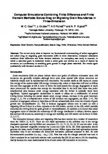
Figure 1.1: NSTAR ion thruster. thrusters use inert gases as propellants. The majority of them use xenon which is a chemically inert, colorless, odorless, and tasteless, noble gas. The first xenon ion thruster ever flown was a Hughes engine launched in 1979 on the Air Force Geophysics Laboratory’s Spacecraft Charging at High Altitude (SCATHA) satellite. The first commercial use of a xenon ion thruster was on PanAmSat 5 (PAS5), a communications satellite launched in August 1997, on a Russian Proton rocket from the Baikonur Cosmodrome in Kazakhstan. These ion thrusters were used for orbit maintenance and station keeping. Ion thrusters for such purposes are smaller than those designed to act as the primary propulsion system during interplanetary missions. In the early 1990’s, NASA initiated the NASA Solar Electric Power Technology Application Readiness (NSTAR) project to develop xenon ion thrusters for deep space missions. The engineering space model of the NSTAR thruster successfully logged more than 22,000 hours (three years) of operation in a vacuum chamber at JPL. The NSTAR thruster, like the one shown in figure 1.1 [49], was used as the primary propulsion system on the Deep Space One spacecraft. On the other coast of the Atlantic, research and development of ion thrusters proceeded in the United Kingdom in two phases. The first phase, from the 1960’s to 1975, resulted in a prototype engine producing 10 mN, in which mercury was used as a propellent. It was proposed to be used for station keeping on Olympus, a large

Raed I. Kafafy


5

research communications satellite. However, due to financial obstacles, the engine did not acquire sufficient laboratory life testing to be flight ready. In the mid 1980’s, work resumed on a new version, which was named UK-10. In UK-10, xenon replaced mercury as a propellant, in order to reduce risks of contamination. UK-10 is a light weight focussed ion beam engine with a 10 centimeter diameter beam. It was developed by the Defence Research Agency at Farnborough, and Matra Marconi Space, with a grant from ESA, and has now had over two thousand hours of life testing, in daily 3 hour pulses, in preparation for space qualification on board the ESA ARTEMIS satellite. UK-10 can achieve up to 70 mN, although it is most efficient at 25 mN. The larger UK-25 ion thruster has achieved a thrust of 260 mN in tests to date. The thrust could probably be extended to 500 mN. These could be used to send fast probes beyond the outer solar system, to near interstellar space, with Delta class rocket’s, at costs within the reach of Discovery class missions now being flown to Mars and the asteroids [23]. Compared with chemical propulsion, the application of ion propulsion in orbit maintenance and station keeping on satellites can lead to a reduction in the propellant utilization by a factor of ten. Considerable gains in payload mass and/or orbital lifetime can be achieved. An example is a low mass, low cost Earth observation satellite which can be orbited at few hundred kilometers, for a lifetime of several years. Launching costs could be greatly reduced by the use of a Pegasus XL launcher followed by orbit raising instead of inserting the satellite directly into orbit. Even more dramatically, the 370 kg Ulysses solar polar satellite, launched in 1989, required an Inertial Upper Stage / PAM combination weighing 20 tons, to place it into orbit. With an ion thruster cluster, the same spacecraft would have required 2.4 tons of engine/propellant, and could thus have been launched by an Ariane 4. It has been calculated that, if the International Space Station were to use ion thrusters for orbit maintenance rather than chemical rockets, about 9 tons of propellant mass per year would be saved which is a considerable cost saving. In a conventional ion thruster, as schematically illustrated in figure 1.2, the propellant is injected into the discharge chamber to be ionized. The conventional method of ionization is called electron bombardment, in which a high-energy electron (negative charge) collides with a propellant atom (neutral charge) to release a second electron, yielding two negative electrons and one positive ion. This ionization process, in a xenon ion thruster, is simply described as: e− + Xe0 → Xe+ + 2e−

Raed I. Kafafy


6

Figure 1.2: A schematic of an ion thruster. Electrons are generated by a hollow cathode, called the discharge cathode, located at the center of the engine on the upstream end. The electrons flow out of the discharge cathode and are attracted to the discharge chamber walls, which are charged to a high positive potential by the thruster’s power supply. High-strength magnets are placed along the discharge chamber walls so that as electrons approach the walls, they are redirected into the discharge chamber by the magnetic fields. By maximizing the time that electrons and propellant atoms remain in the discharge chamber, the chance of ionization is maximized and hence the efficiency of the ionization process. An alternative method of ionization called electron cyclotron resonance (ECR) is also being researched at NASA. This method uses high-frequency radiation (usually microwaves), coupled with a high magnetic field to heat the electrons in the propellant atoms, causing them to break free of the propellant atoms, creating plasma. Ions can then be extracted from this plasma. The ions produced in the discharge chamber are accelerated by electrostatic forces. The electric fields used for acceleration are generated by electrodes positioned at the downstream end of the thruster. Each set of electrodes, called ion optics or grids, contains thousands of coaxial apertures. Each set of apertures acts as a lens that electrically focuses ions through the optics. NASA’s ion thrusters use a two-electrode system, where the upstream electrode (called the screen grid) is charged highly pos-

Raed I. Kafafy


7

itive, and the downstream electrode (called the accelerator grid, or accel grid) is charged highly negative. Since the ions are generated in a region of high positive potential and the accelerator grid’s potential is negative, the ions are attracted toward the accelerator grid and are focused out of the discharge chamber through the apertures, creating thousands of ion jets. The stream of all the ion jets together is called the ion beam, whereas the stream of an individual ion jet is called a beamlet. The exhaust velocity of the ions in the beam is based on the voltage applied to the optics. While a chemical rocket’s top speed is limited by the thermal capability of the rocket nozzle, the ion thruster’s top speed is limited by the voltage that is applied to the ion optics. Efficiency and thrust are determined by ionization voltage from anode to cathode, and by propellant feed rate. Typically, ionization voltages of over 40 volts lead to erosion of the thrust chamber and reduced life span, while fuel utilization rates of 6 milligrams per second produce 25 mN, within a field of 1100 volts. Because the ion thruster expels a large amount of positive ions, an equal amount of negative charge must be expelled to keep the total charge of the exhaust beam neutral. A second hollow cathode called the neutralizer is located on the downstream perimeter of the thruster and expels the needed electrons [48].

1.2.3

Ion Thruster Lifetime and Failure Modes

The lifetime of an ion thruster is primarily limited by the erosion of thruster components, especially the ion optics [37]. Currently, the ion optics grids of nearly all ion thrusters are made of molybdenum (Mo). The use of carbon-based ion optics (CBIO) has been shown to sufficiently suppress the erosion of the screen electrode as to effectively remove sputter erosion of that electrode as a failure mechanism. However, the reduced erosion rates of the accel electrode will remain one of the principal thruster life-limiters. Charge-exchange (CEX) ions play a profound role in the erosion of the accel grid. CEX ions result from the CEX collisions between fast beam ions and slow propellant neutrals according to the following reaction + Xeslow + Xe+ f ast → Xeslow + Xef ast

The erosion of the accel electrode by CEX ions can be related to three mechanisms [90]:

Raed I. Kafafy


8

• the erosion of the downstream face of the electrode by ions with energies comparable to the accel electrode potential (a few hundred Volts) that form a pit and groove pattern, • the erosion of the upstream side of the electrode by ions with energies comparable to the total accelerating voltage (up to 10 kV), and • the erosion of the aperture walls by ions which have energies varying between the total voltage and the accel voltage. Electrode failure by pit and groove erosion occurs when the grooves wear through the electrode causing structural and/or electrical failure. Electrode failure due to impingement on the upstream surface of the accelerator grid occurs at the onset of electron backstreaming. Either thinning of the electrode or aperture enlargement once the erosion pattern has worn through can lead to electron backstreaming. Failure resulting from aperture enlargement due to the third mechanism can occur either by electron backstreaming or structural failure. Structural failure due to aperture enlargement occurs when the aperture diameter reaches the groove of the pit and groove erosion.

1.2.4

Spacecraft-Ion Thruster Interaction and Integration Problems

Thruster plume is one of the major sources of spacecraft contamination. Thruster exhaust products may backflow towards spacecraft surfaces by several mechanisms. In the case of ion thruster plume, Wang et. al. [80] showed that the the CEX ions backflow through an expansion process which is similar to the expansion of mesothermal plasma into vacuum. The electric field established by the CEX plasma around the spacecraft also controls the trajectories of the ionized contaminants. Contaminants that adhere to the surface can either condense or be absorbed onto the surface. Condensation can be a very serious problem because it easily forms a thick layer on a surface. It is usually avoided on spacecraft surfaces by using materials that emit a very small fraction of volatile condensible material (VCM). After VCMs, the main source of deposition on spacecraft surfaces is adsorption of individual molecules. An adsorbate forms because of surface attraction between individual atoms of the substance and those of the contaminant. The degree of adherence of any individual particle depends on the gas species, the surface temperature, the composition of the

Raed I. Kafafy


9

substrate, and the amount of surface coverage. As a monolayer is completed, the likelihood decreases that additional contaminant molecules will stick because they will not see any substrate molecules [24]. The presence of a thin contaminant film on the surface of a material will alter its solar absorptance. The contaminant layer will increase the absorptance of the surface material and consequently its equilibrium temperature [74]. In addition to the concern of contamination of thermal control surfaces, there is also the possibility for contamination buildup on optics or solar arrays. The presence of a contaminant film on a lens, mirror or focal plane will degrade the signal to noise ratio (SNR) of the detector and limit the dynamic range by absorbing light from the target of interest. If the contaminant film becomes too thick, the sensor will cease to function properly [74].

1.3

Modeling Ion Propulsion

The modeling of ion propulsion started a few decades ago even before the development of the first ion thruster prototype during the 1950’s by Harold Kaufman. Simple analytical and/or numerical methods were applied to model the performance of ion thrusters including such useful information as the thrust, current, divergence angle [25]. Also, other simplified and/or numerical studies have been performed to investigate the motion of CEX ions, as well as their effects on both ion thruster grid surfaces and spacecraft critical components as a whole. Despite their success to give a qualitative insight on ion thruster operation such models were incapable of predicting CEX ion sputtering and deposition rates for arbitrary geometries and operating conditions [56]. Starting in the 1990’s, the Particle-In-Cell (PIC) method [7] has been applied to model ion optics as well as ion thruster plume. PIC models are more appropriate for these applications because the mean free path length λmf p for both ion optics and plume problems is very large as compared with the characteristic system dimensions. The mean free path length is given by λmf p =

1 nσ

where n is the plasma density and σ is the collision cross-section associated with a certain collision mechanism. For a typical ion thruster, σ is in the order of 10−20 m2

Raed I. Kafafy


10

and n ranges from 1016 m−3 to 1018 m−3 for the inside plasma and from 109 m−3 to 1012 m−3 for the outside plasma. This results in λmf p ranging from 102 m to 104 m for the inside plasma as compared with the millimeter dimensions of the ion optics apertures, and from 108 m to 1011 m for the outside plasma as compared with the few meters dimensions of the spacecraft. In a PIC model, real plasma particles are represented by much fewer simulation particles. A typical computational cycle includes four steps: 1) particle push, 2) charge deposit, 3) field solve, and 4) force weigh. The space charge, particle trajectories and electric fields are solved self-consistently. The PIC model applies linear schemes to deposit, or interpolate, the charge of moving particles to the discrete mesh nodes, and weigh, or interpolate, the electric fields from mesh nodes to particle positions. The details of the PIC model will be discussed in chapter 5. Numerical accuracy and computational efficiency lead to contradicting requirements in the design and implementation of PIC models. The PIC models that are currently used in ion propulsion simulations are either based on finite difference methods or standard finite element method. A detailed literature review will be provided in chapter 2.

1.4

Motivation

Ion propulsion development is increasingly dependent upon inputs from physics based modeling. In order to apply the particle simulation method as a research tool, one needs to build a code that is sophisticated enough so that complex geometric and field effects can be modeled properly, and yet computationally efficient enough so that large-scale particle simulations can be performed routinely within reasonable time. Because of these conflicting requirements for an accurate field solver and a fast particle pusher, the plasma-material interface represents a major challenge in the application of PIC codes for ion optics modeling [35] as well as spacecraft-ion thruster interaction modeling [80]. In this study, we aim at developing a numerically accurate and yet computationally efficient simulation algorithm which we apply to simulate the main physical phenomena occurring during the operation of an ion thruster such as beam extraction and CEX ions and spacecraft contamination by the ion thruster plume species.

Raed I. Kafafy

1.5


11

Research Objectives

The objective of this research is to develop a three-dimensional immersed finite element (IFE) method. This method is designed to be capable of retaining second order accuracy while solving an interface boundary value problem (BVP) on a regular, even Cartesian domain. Based on the three-dimensional IFE method, we develop a three-dimensional (IFE) field solver for plasma simulation applications. The most attractive advantage of the new field solver is that it can solve the interface field boundary value problem on a Cartesian-based tetrahedral mesh irrespective of the shape and position of the interface. It can also be used to investigate the effect of involving materials with different dielectric constants since it incorporates explicitly the material properties in the field solution. Next, we integrate the IFE field solver to a Cartesian-grid PIC code which is modified from a legacy standard PIC code. It is well known that Cartesian-grid PIC codes are very fast in performing particle-mesh interpolations and particle pushing. We further adopt a new meshing technique in particle simulation in which we let the PIC and IFE mesh nodes to be dislocated. This allows us to stretch the IFE mesh according to the local potential gradients and plasma conditions while retaining the ultimate speed of a uniform Cartesian grid PIC code. The target of the new PIC model is large scale electrostatic plasma simulations which involve complex geometries such as those encountered in ion optics and spacecraft-ion thruster interaction problems.

1.6

Organization of the Dissertation

This dissertation is arranged in 8 chapters. The description of these chapters is as follows Chapter 1 is an introduction in which we introduce the background and motivation for this research work. We also briefly describe our contribution. Chapter 2 is a literature review of the research work which has been done prior to the current research work. Because of the nature of the current work, the literature review includes three parts: numerical methods to solve the field equation on irregular boundaries, ion optics modeling, and spacecraft-ion thruster interaction modeling.

Raed I. Kafafy


12

Chapter 3 is the theoretical development of the three-dimensional immersed finite element (3D IFE) method. In this chapter, we also present a numerical error analysis of the method developed. Chapter 4 presents the details of the IFE field solver that is used in all IFE–PIC simulations in the current work. Chapter 5 introduces the Hybrid-Grid Immersed-Finite-Element Particle-In-Cell (HG-IFEPIC) model. The details of the model are discussed. Numerical experiments showing the approximation capabilities of the model are also presented. Chapter 6 introduces the physical and mathematical modeling of the NEXT ion optics. It also presents the results of the ion optics simulations performed at selected operating conditions. Chapter 7 introduces the modeling of the spacecraft-ion thruster plume interactions. It also presents the simulation results obtained for selected spacecraft-ion thruster configurations and firing options. Chapter 8 contains conclusions and a discussion of the results obtained in the current work. It also summarizes the scientific contributions made to the corresponding disciplines of science and engineering. This chapter also introduces the future research work that is recommended by the author.

Chapter 2 Literature Review 2.1

Introduction

The literature review, herein, is organized into three sub-reviews, to cover the different aspects of this study: • A review of the ion optics models, • A review of the spacecraft–ion thruster plume interactions models, and • A review of the field solution methods for problems involving complex boundaries. The first section reviews the research work conducted in ion optics simulations during the last decade (1994-2005). The next section reviews the main research work contributing to simulation of spacecraft-ion thruster plume interactions during the last decade as well. Starting in the 1990’s, the Particle-In-Cell (PIC) method [7] has been widely applied to model ion optics as well as spacecraft ion thruster plume interactions. The third section reviews the research work performed to develop numerical methods that are capable of accurately handling elliptic problems with complex boundaries.

13

Raed I. Kafafy

2.2

Chapter 2. Literature Review

14

Previous Work On Ion Optics Simulation – Review of the Last Decade

During the last decade, many research work has been conducted to numerically study the ion optics problem. In the following, we introduce a review of most of the work done in a chronological order. In 1994, Peng et al. [57] In developed a particle simulation code to study ion optics and the effect of charge-exchange-induced grid erosion in electron bombardment ion thrusters. The code is based on particle-in-cell (PIC) and direct simulation Monte Carlo (DSMC) methods. Two versions of the code were tested. A two-dimensional axisymmetric code was presented to run on PCs. They also developed a threedimensional code in which they showed the necessity to calculate the pitted erosion patterns observed in ground tests. In 1996, Arakawa and Nakano [1] developed a three-dimensional optics code to calculate both beam divergence and ion-sputtering rate to grids due to charge-exchange. In the code, the simulation domain does not extend from the upstream ion sheath region to the downstream plasma. Instead, they assume an emitting surface for the ions. The position and shape of the emitting surface are initially guessed then they are iterated on during computations till convergence using the distance between the lower and higher potentials as obtained by the space-charge-limited current law (Child’s Law). This leads to a reduction in memory storage and computation time by avoiding the meshing of the upstream plasma region in which mesh size is limited by the local Debye length. Therefore, their code can be run within a reasonable time on PCs. Although the code is more efficient concerning the memory storage and computational time, the results obtained depend on the accuracy of the ion trajectories which is degraded by the inaccuracy in predicting the shape and position of the emitting surface. In 1998, Tartz et al. [73] presented a two-dimensional, axisymmetric simulation code that can be used to tackle a comprehensive optimization of a grid system in a rather short computational time even on a PC. In their approach to the modeling of the broad beam formation and secondary grid-eroding impact of charge-exchange ions, they break down the complex interaction pattern into a series of largely independent processes, leading to a considerably reduced computational effort. The extraction of ions, calculation of potential, and ion trajectories are done self-consistently using IGUN [6]. They also tried to take into account the effect of neighboring holes on the simulated hole by estimating their influence in the two-dimensional simulations

Raed I. Kafafy


15

in a spherical approximation assuming a ring-shaped aperture. In 1999, Muravlev and Shagayda [46] developed a two-dimensional planar and axisymmetric code to be used in the simulation of ion thruster extraction grid performance and erosion process. They presented a simplified approach to predict the erosion pattern without fully three-dimensional modeling. In such approach, they used a standard computational domain with a cross-section of a 30 by 60 degrees triangle. The trajectories of both the charge-exchange ions and downstream plasma ions are calculated with three spatial components. The axial and radial components are determined from the two-dimensional results. The azimuthal component is assumed to be zero. They also studied both circular and slit apertures. In 1999, Okawa and Takegahara [51] presented a two-dimensional axisymmetric particle simulation code with three-dimensional velocity components to investigate the beam extraction phenomena from a discharge plasma. They treated electrons as particles as well as ions. Though, the simulation was preliminary, they could estimate the position and shape of the plasma sheath boundary. In 2000, Boyd and Crofton [9] performed a computational study on grid erosion through ion impact. Their model employs a combination of a hybrid fluid-PIC method for the plasma dynamics, and a DSMC method for collision dynamics involving momentum transfer, charge exchange, and Coulomb collisions. In the model, both single and double charge ions are treated as particles. Comparing results with experimental measurements of grid currents for the UK-T5 ion thruster, the model accurately predicts the current collected on the acceleration grid for a range of operating points. However, it significantly under predicts the current collected on the deceleration grid. In 2001, Nakayama and Wilbur [47] performed a numerical study on a high-specific impulse many-grid ion thruster operated at a voltage of 10 kV. In the study, they used a three-dimensional particle simulation code that employs an energy compensation method, a simplified pre-sheath method, and high-speed coding. In the study, they modified the OPT code which is a two-dimensional cylindrical ion optics code. They also developed the igx code, which is a three-dimensional ion extraction simulation code. In 2001, Wang et al. [88, 89] developed a fully three-dimensional particle simulation mode for ion optics. The model allows multiple apertures to be included explicitly in the simulation domain and makes no assumptions on the upstream sheath. Simulation results show both qualitative and quantitative agreement with experimentally observed erosion patterns in the NSTAR ion thruster. In the model, the

Raed I. Kafafy


16

three-dimensional optics aperture geometry is handled by a method of sub-grid scale placement of boundaries which explicitly includes the location of the optics wall in relation to the grid in the finite difference formulation of the Poisson’s equation. In 2002, Wang and Lin [86] developed a two-dimensional axisymmetric electric field solver for ion optics modeling. The solver is based upon the two-dimensional, axisymmetric immersed finite element (IFE) method. The IFE method is believed to provide a very promising tool to tackle ion optics simulation problems that involve complex geometries on Cartesian meshes. So, computational speed doesn’t have to be sacrificed in favor of accuracy. In 2003, Farnell and Wilbur [20] presented simulations of the grid erosion processes for two proposed sets of ion thruster grids for the NEXT project. They discussed structural failure and electron backstreaming due to acceleration grid erosion as two possible failure mechanisms. The ffx was used in the simulation. It is a threedimensional, Cartesian optics code, extended from the igx code with additional features such as the ability to model a wide range of grid geometries including cusp details and mis-aligned aperture pairs. The simulation is applied to a two, quartersized apertures in a hexagonal aperture layout. The field is solved using a relaxed Gauss-Seidel multigrid method. Erosion of a cusped grid geometry was simulated using checker-board like simulation geometry. More details about the ffx code can be found in [21]. In 2003, Emhoff and Boyd [17] presented a computational study of the NEXT ion thruster optics. The optics code they used provides a two-dimensional axisymmetric simulation of a single aperture on a uniform Cartesian grid. The code uses a PIC method to simulate Xe, Xe+ and Xe++ and the DSMC method for processing the particle collisions. They explored the dependence of the accelerator grid current on downstream domain length and suggested an improving method. They also studied the effect of beam voltage on accelerator grid aperture wall erosion and performed life estimates for both cusped and non-cusped optics geometries. In 2003, Kafafy and Wang [34] developed a fully three-dimensional ion optics simulation code, the IFE–PIC, which is based upon a standard PIC code and adopts the recently developed three-dimensional IFE method. The developed three-dimensional IFE field solver demonstrated very good agreement with field solutions obtained by r highly accurate finite element solvers such as FEMLab by the MathWorks Inc. The ion optics simulations also show good agreement with simulations obtained by Wang’s ion optics simulation code [89], which was validated by experimental results. In 2004, Emhoff and Boyd [18] presented a numerical study to characterize the error

Raed I. Kafafy


17

associated with the solution of the field equation. They suggested an improved twodimensional axisymmetric field solver in which the potential mesh was refined to reduce numerical errors. For a two-dimensional single aperture domain, the most refined simulation takes over 8 hours on a 3.06 GHz PC, which makes the technique prohibitively impractical for three-dimensional simulations. In 2004, Farnell [19] used the ffx code to investigate the lifetime and propellant throughput capability of the High Power Electric Propulsion (HiPEP) thruster ion optics. Erosion predictions are presented as a function of beamlet current, accel grid voltage, and propellant utilization efficiency. He also performed a design parametric study in which design parameters were varied in a systematic manner to assess their effect on beamlet current limitations and electron backstreaming margins. In 2004, Kafafy and Wang [35] introduced the hybrid-grid IFE–PIC (HG–IFE– PIC) code which is an extension to the IFE–PIC code. The HG–IFE–PIC code uses two different meshes for particle simulation and field solution. The PIC mesh is a uniform Cartesian mesh which retains the simplicity and speed of a standard PIC code, while the IFE mesh is a multi-zone stretched Cartesian-based tetrahedral mesh which has much less number of nodes and elements than a uniform IFE mesh. They used the HG–IFE–PIC code to study the ion optics of a subscale gridlet in a domain that includes three non-similar apertures for the first time ever. The details of the HG-IFE-PIC model and the new meshing technique is discussed in chapter 5, while the details of the ion optics simulations is given in chapter 6. In 2005, Kafafy et al. [33] applied the HG-IFE-PIC code to investigate the dynamic behavior of beam ions in NEXT ion optics. The code was used to span the ion optics operation envelope from cross-over up to perveance. The cross-over limit predictions were in a reasonable agreement with experimental data.

2.3

Previous Work On Spacecraft–Ion Thruster Plume Interaction – Review of the Last Decade

In this section, we present a chronological review of the research work performed in the last decade to investigate the aspects of the spacecraft–ion thruster plume interactions through physical and numerical modeling. In 1995, Wang and Brophy [82] developed a 3D particle-in-cell Monte-Carlo collision simulation model for ion beam-spacecraft plume interactions and presented

Raed I. Kafafy


18

simulation results for ion beam emissions under various charging conditions. They found that when the interaction is within the low-charging regime, such as that of an ion propulsion application, interactions are primarily due to the charge-exchange ions; these typically do not alter the spacecraft’s charging environment. They also noted that ion beam emissions in the high-charging regime may be used to efficiently discharge a spacecraft. In 1996, Samanta Roy et al. [67, 68] developed a two-dimensional axisymmetric physical and numerical model to investigate the plasma environments induced by an ion thruster and to assess plume backflow contamination. The model takes into account five components of the thruster effluents; propellant beam ions, propellant neutrals, propellant CEX ions, non-propellant efflux neutrals and CEX ions, and electrons. They applied the model to predict the propellant CEX plasma and sputtered Mo-grid metal efflux from the NASA 30-cm ion thruster (NSTAR) over a wide range of operating conditions. They also showed that the ratio of the propellant Xe ions to sputtered Mo ions is not constant throughout the backflow region. The Mo deposition predicted was less than what was previously expected. In addition, they examined the sensitivity of the plume backflow to the beam electron temperature and found they are strongly correlated. Finally, they evaluated the application of an optional plume shield which was found to be effective in reducing the backflow for the two-dimensional model they studied. In 1996, Samanta Roy and Hastings [66] also developed a three-dimensional model to study the composite plume backflow of two 8-cm ion thrusters. The resulting potential structure was found to trap the propellant CEX ions and introduce a preferred ejection direction, whereas, it had a little effect on the sputtered grid material due to its higher initial energy. They concluded that the net backflow of dual thrusters is not a simple superposition of the backflow from two single thrusters. In 1996, Samanta Roy et al. [69] developed a fully three-dimensional hybrid plasma particle-in-cell model for multi-computer environments to assess the spacecraft backflow contamination of an ion thruster. They presented results of plume backflow for a 13-cm Xenon ion thruster operating with a current level of 0.4 A on a model spacecraft. The computational domain was over 40 m3 in volume and contained 9.4 million grid points, and the number of simulation particles used was over 35 million representing CEX Xe ions produced in the plume. In their calculations, they used a massively parallel 256-node Cray T3D. However, the spacecraft model that was studied was oversimplified because of numerical constants such that it was lacking many of the important geometric details of a real spacecraft.

Raed I. Kafafy


19

In 1997, Wang et al. [83] developed a global analysis of ion thruster plume interactions for interplanetary spacecraft based on fully three-dimensional electrostatic particle-in-cell Monte-Carlo simulations of the near-field region and 2 12 –dimensional electromagnetic hybrid PIC simulations of the far-field region. They showed that while the charge exchange ion interaction dominates in the vicinity of the spacecraft, the presence of the solar wind will induce kinetic couplings between the plume and the solar wind in the far-field via electromagnetic plasma instabilities. The instabilities can generate enhanced magnetic field fluctuations leading to wave-particle scatterings of both the beam ions and the CEX ions. In 1999, Gardner and Katz [22] developed a parametric model of an electric propulsion plume including primary beam and line-of-sight ions and hollow cathode neutralizer ions. They also modeled plume optical irradiance spectra and line-of-sight intensities. The Environment Work Bench (EWB) was used to implement the models. They performed calculations to compare the thruster plumes for both the Deep Space–1 30-cm ion thruster and the SPT-100 stationary plasma thruster. They presented preliminary results and discussed the models, testing and analysis required to understand the impact of the mentioned thrusters on spacecraft subsystems. In 1999, VanGilder et al. [77] presented a two-dimensional axisymmetric hybrid Monte Carlo particle-in-cell code to simulate the plumes of ion thrusters and Hall current thrusters. The code employed two different grids; an unstructured grid used by the Direct Simulation Monte Carlo (DSMC) code and a non-uniform Cartesian grid used by the PIC code. The authors compared the computed flow field results with the existing experimental measurements for the UK-10 ion thruster which consisted of ion flux, ion density, and floating potential data. Xe neutrals and ions were modelled directly, while electrons were described by Boltzmann law. They included the effect of finite back pressure. They noticed high sensitivity of simulation results to input conditions assumed at the thruster exit plane, particularly the uncertainty in specifying the effects of the curvature of the dished grids of the UK-10 thruster on the exit ion velocity profile. They also studied the sensitivity of simulations to certain parameters including; the cross-section of CEX reactions, the mechanics of CEX reactions, and the electron temperature. They found that the beam ions are only moderately dependent on variations in these parameters, whereas the CEX ions are sensitive to them. In 2001, Wang et al. [80] developed a three-dimensional particle-in-cell model to compute the ion propulsion induced plasma environment for the Deep Space 1 (DS1) spacecraft. They compared simulations with in-flight measurements of CEX plasma from the ion propulsion diagnosis subsystem (IDS) on DS1. It was found that the

Raed I. Kafafy


20

plasma from the plasma environment of DS1 is dominated by the CEX plasma from the plume. They found that the CEX plasma near the spacecraft surface, for a typical thruster operating conditions, had a density ranging from 106 cm−3 near the thruster to 104 cm−3 at the opposite end of the spacecraft surface and a current density ranging from 10−7 A/cm2 to 10−9 A/cm2 . They also showed that, for an interplanetary spacecraft and a moderate charging potential, CEX ion backflow goes through an expansion process similar to that of mesothermal plasma into a vacuum or plasma wake. They also noted that since the spacecraft potential is shielded by the thin propellant CEX plasma sheath, it does not have any significant effect on the backflow of the ionized Mo particles sputtered from the thruster. In 2003, Wang et al. [78] developed a three-dimensional PIC model which incorporates the immersed finite element (IFE) method for plasma particle simulations. The major advantage the IFE-PIC model for simulations involving complex geometric boundary conditions is to allow the direct usage of standard Cartesian mesh-based algorithms for particle pushing regardless of the geometry of object boundaries. The IFE formulation also allows material properties to be included explicitly and maintains the desired physics at the given material interface. Preliminary results were presented therein. In 2004, Mandell et al. [44] presented a two-dimensional axisymmetric plume model of a 30-cm ion engine, operating at high jet power (>20 kW). The model accounted for the main ion components expected to be present in the thruster plume, namely main beam ions and ion products from ion-neutral scattering. They found main ions within ∼30 deg of the beam axis of symmetry, and have energies in excess of 3000 eV and peak densities in the order of 1015 m−3 near the thruster exit. CEX ions are expelled radially from the main beam due to their low energies (70 deg). Ions that are elastically scattered were found to retain most of the initial kinetic energy (100-3000 eV) and were found with peak densities in the order of 1012 m−3 and populate the complete range of plume angles. In their simulations, they used the EPIC/Plume tool. In 2004, Wang et al. [79, 11] introduced a prototype virtual laboratory for spacecraft plasma interactions and electric propulsion. This virtual laboratory consists of a simulation engine and a virtual testing environment. A user provides physical parameters and spacecraft configurations to the simulation engine. The virtual laboratory simulates the physical processes using a set of particle simulation codes and then displays the results in a virtual testing environment using immersed and/or collaborative visualization. They developed a new particle simulation code, DRACO, for plasma simulations involving complex boundary conditions. DRACO incorpo-

Raed I. Kafafy


21

rates the IFE–PIC algorithm. This method allows one to use a Cartesian mesh to handle complex geometric or time-varying interface between plasma and object without scarifying the accuracy in electric field solutions. In 2004, Wang and Kafafy [84] used the IFE–PIC code to study the interaction of multiple ion thruster plumes with spacecraft. They studied three configurations of ion thrusters; a single thruster, three in-plane thrusters, and an array of four parallel thrusters. The thrusters in each configuration were given major possible firing options. They showed the dependence of the near-spacecraft plasma environment on spacecraft-thruster configurations and firing options. They also assessed the contamination of solar arrays by ion thruster operation for each configuration and thruster fining option. The details of this work will be provided in chapter 7.

2.4

Review On Methods To Solve A Field Problem With Complex Boundaries

The electrostatic field problem with complex boundaries may be, in general, described by a Poisson’s equation with discontinuous coefficients. This equation appears in many scientific and engineering applications which includes, but is not limited to, fluid mechanics, electromagnetics, heat transfer, biomechanics as well as plasma physics. It is well known that the solution of such equation not only slows down the entire simulation for many applications, but also leads to loss in accuracy. Solving interface problems efficiently and accurately is still a challenge because of many irregularities associated with them [41]. In order to overcome the obstacles in solving Poisson’s equations with discontinuous coefficients, many numerical methods have been developed. In the following, we present a brief review on the numerical methods which are closely related to the IFE method. We classify these methods similar to [41] as; • body-fitting-grid methods discretization • Cartesian-grid methods based on finite difference discretization • Cartesian-grid methods based on finite element discretization

Raed I. Kafafy

2.4.1


22

Body-Fitting-Grid Methods

It is well known that a second order accurate approximation to the solution of an interface problem can be generated by the Galerkin finite element method with the standard linear basis functions if the triangulation is aligned with the interface, i.e. body fitting grid, [4, 10, 16]. One advantage of the finite element formulation is that the resulting linear system of equation is symmetric positive definite for a self-adjoint elliptic operator which ensures the stability of the algorithm. It is also possible to produce second order accurate approximation to the solution of the interface problem by applying the appropriate second order accurate finite difference schemes in a bodyfitting curvilinear grid [85]. Disadvantages of Body-Fitting-Grid Methods It is difficult and time consuming to generate a body fitting grid for an interface problem in which the interface separates the solution domain into pieces or problems with complicated geometries. Such a difficulty becomes even more severe for moving interface problems because a new grid has to be generated at each time step [41, 15]. Other concerns are raised by particle simulation models. Particle simulation models using body-fitting grids usually put an annoying computational over-head to search for particles using cumbersome techniques [27]. Such complicated particle search techniques slow down the whole simulation and/or limit the size of the problems that can be handled. Advantages of Cartesian-Grid Methods The advantages of using a Cartesian grid or an adaptive Cartesian grid method to solve an interface problem is summarized below [41, 15]: • Grid generation is trivial and almost costless. This becomes much more significant for moving boundary/interface problems. • Many efficient and popular packages/solvers and numerical methods are available for Cartesian grids. For example, fast Poisson solvers such as fishpack, Navier-Stokes equation solvers in two and three dimensions on a rectangular square or a box, Clawpack for conservation laws, and FFT packages etc. It

Raed I. Kafafy


23

is relatively easier to incorporate new methods using existing packages/solvers based on the same grid. • The level set method, which has been successfully used to treat a number of moving interface/boundary problems, especially for problems with topological changes, and for problems in three dimensions - works best with Cartesian grids. • Construction of super convergent approximations to important physical quantities such as fluxes is much easier using Cartesian grids.

2.4.2

Cartesian-Grid Methods Based On Finite Difference Discretization

The numerical methods based on Cartesian grids may have some difficulties that need to be overcome and may lose accuracy as well for curved interfaces/boundaries. Due to non-smoothness of the solutions, many standard finite difference methods do not apply for interface problems. A huge research effort has been made regarding these problems. In the following, we will only review most of the methods which are related to this work. The Immersed Boundary Method (IBM) Peskin [58] introduced the immersed boundary method in 1976 . The method was designed to solve problems of biological fluid mechanics which often involve the interaction of a viscous incompressible fluid with an elastic membrane which can be considered as a boundary immersed in the fluid. The main idea of the method is to use a regular Eulerian computational grid for the fluid mechanics together with a Lagrangian representation of the immersed boundary. The immersed boundary exerts a singular force on the fluid and at the same time moves at the local fluid velocity. The interaction between the fluid and immersed boundary can be modeled by a well chosen discretized approximation to the Dirac delta function, which is called a discrete delta function. This approach has been applied successfully to problems of blood flow pattern in the heart, wave propagation in the cochlea, flow in collapsible tubes, aquatic animal locomotion, platelet aggregation during blood clotting, the flow of suspensions, flow and transport in a renal arteriole, and the cell and tissue

Raed I. Kafafy


24

deformation under shear flow [38]. However, the IBM is designed for problems with only a singular source term and continuous coefficients. The Level Set Method (LSM) Osher and Sethian [54] first proposed the level set method in 1988. The method has been successfully used to treat a number of moving interface/boundary problems, especially for problems with topological changes, and for problems in three dimensions. The advantage of the level set method is that one can perform numerical computations involving curves and surfaces on a fixed Cartesian grid without having to parameterize these objects (this is called the Eulerian approach). The level set method works best with Cartesian grids. The Smoothing Method for Discontinuous Coefficients Sussman et al. [71] introduced in 1994 a simple approach to adopt the level set method by smoothing out the coefficient. The level set expression of interfaces makes the smoothing method much easier for two and three dimensional problems. However, solutions are also smeared out by the smoothing method. The Immersed Interface Method (IIM) LeVeque and Li [43] introduced the immersed interface method (IIM) in 1994. The motivation was to develop a second-order accurate finite difference scheme for elliptic equations which may have discontinuous coefficients, or singular sources along a general interface, externally imposed constraints in the jump of the solution or its normal derivatives across an interface. The method was successful in applications to one-, two- and three-dimensional problems; elliptic, parabolic, hyperbolic, and mixed type equations; fixed and moving interfaces, and many applications [40, 15]. However, the resulting linear system of equations is not symmetric positive definite. In addition, the method is not very robust, because the stability of the algorithm may depend on the choice of one or more additional grid points in addition to the standard finite difference scheme.

Raed I. Kafafy


25

The Embedded Curved Boundary Method (ECB) Hewett [27] introduced the embedded curved boundary method (ECB) in 1997. The method was intended to incorporate piecewise-linear approximations to curved boundaries for codes that use orthogonal meshes. The ECB is designed to retain much of the fidelity of unstructured-grid methods while retaining simplicity and run time advantage of orthogonal mesh based codes. This method provides a practical approach to problems such as space charge emission. However, the resulting linear system of equations from this method is also not symmetric positive definite; a property that is very favorable for the stability of the solution.

2.4.3

Cartesian-Grid Methods Based On Finite Element Discretization

The Partition of Unity Method (PUM) A new generalized finite element method that was presented by Babuˇska and Melenk [5] in 1997. This method features the ability to include in the finite element space knowledge about the partial differential equation being solved. In addition, finite element spaces of any regularity can be constructed very easily. The PUM method underlies many of the other finite element methods and can be considered as a generalization of the h and p version of the finite element method which underlies many of the finite element methods developed earlier. Although, the PUM does not present a specific set of finite element methods that are suitable for each situation, many finite element methods that have been developed later to address specific problems much more efficiently have followed the same approach of the PUM. The Extended Finite Element Method (X-FEM) Sakumar et al. [64] introduced the extended finite element method in 2000. This method was designed specifically to model cracks in three-dimensions. In this method, a discontinuous function and the two-dimensional asymptotic crack-tip displacement fields are added to the finite element approximation to account for the crack using the notion of partition of unity. The additional functions are used to model the presence of cracks, voids or inhomogeneities, and also to improve the accuracy in problems where aspects of the functional behavior of the solution field is known a

Raed I. Kafafy


26

priori. The Immersed Finite Element Method (IFE) Lin et al. [42] introduced the immersed finite element method in 2001. The method constructs a rectangular finite element space based on rectangular elements to be used for the solution of boundary value problems with discontinuous coefficients. The basis functions in this space are constructed to satisfy the interface jump conditions either exactly or approximately. Such interface problem is involved in many applications such as the projection method for solving Navier-Stokes equations involving two-phase flow, the Hele-Shaw flow and many others. In 2003, Li et al. [41] extended the method to include triangular elements. They also considered both nonconforming and conforming finite element spaces. The corresponding interpolation functions of the method was proved to be second order accurate in the maximum norm. However, the IFE method proposed was only appropriate for two-dimensional and axisymmetric problems. Recently, Kafafy et al. [32] extended the IFE method to involve the solution of essentially three-dimensional problems by constructing the appropriate three-dimensional finite element space based on tetrahedral elements. Details of the development of the three-dimensional IFE method, properties of the finite element space, and numerical examples are given in chapter 3. Immersed Finite Element Method (IFEM) Zhang et al. [93] presented the finite element method in 2004. This method was proposed for the solution of complex fluid and deformable structure interaction problems encountered in many physical phenomena. In this method, a Lagrangian solid mesh moves on top of a background Eulerian fluid mesh which spans over the entire computational domain. Both fluid and solid domains are modelled with the finite element methods and the continuity between the fluid and solid sub-domains are enforced via the interpolation of the velocities and the distribution of the forces with the Reproducing Kernel Particle Method (RKPM) delta function. The higher-ordered RKPM delta functions enables the fluid domain to have nonuniform spatial meshes with arbitrary geometries and boundary conditions. This method was mentioned here because it shares the same name as the finite element methods presented in this work, although they follow different approaches and target different applications.

Raed I. Kafafy

2.5


27

Contribution

Reviewing the current plasma simulation codes that are used for ion optics and ion thruster–spacecraft interactions, we found that most of them are incapable of resolving the complex effects of realistic geometries in large-scale simulations. Most of these codes use standard finite difference field solvers which are known to lose accuracy in the vicinity of geometric boundaries and interfaces, if not carefully adjusted which is mostly the case. Body-fitting grid finite element particle-in-cell codes are very accurate, but much time consuming. Therefore, they are limited to small size problems. In this research, we develop a three-dimensional immersed finite element method, which we use to build a three-dimensional immersed finite element (IFE) field solver. The most attractive advantage of the IFE solver is that it can solve the interface field boundary value problem on a Cartesian-based tetrahedral mesh irrespective of the shape and position of the interface. It can also be used to investigate the effect of involving materials with different dielectric constants since it incorporates explicitly the material properties in the field solution. Next, we integrate the IFE field solver to a Cartesian-grid particle-in-cell (PIC) code which is modified from a legacy standard PIC code. It is well known that Cartesiangrid PIC codes are much very fast in performing particle-mesh interpolations and particle pushing. We use the resulting IFE–PIC code in doing ion optics simulations as well as ion thruster–spacecraft interaction simulations. We also introduce a novel meshing technique in particle simulation codes. In this technique, we generate two separate meshes; a uniform Cartesian mesh for the PIC code and a multi-zone stretched Cartesian-based tetrahedral mesh for the IFE field solver. The uniform Cartesian PIC mesh retains the maximum speed of a standard PIC code, whereas the multi-zone stretched Cartesian-based tetrahedral mesh provides the required mesh refinement for accurate field solution avoiding computational and storage burden caused by IFE mesh over-refinement. Ion optics simulations are performed on the NEXT ion optics using the HG-IFE-PIC Ion Optics model to assess the ion extraction capabilities as well as the impingement current and electron backstreaming limits. In addition to the standard HG-IFE-PIC Ion Optics model, we introduce a Streamline HG-IFE-PIC Ion Optic model which is meant to be much faster and less memory consuming. We perform ion optics simulations in a two-quarter aperture domain as well as a whole ion optics gridlet seven-aperture domain. Since similarity among all apertures in a subscale gridlet

Raed I. Kafafy


28

can not be clearly justified for such a small number of apertures, it may be necessary to incorporate all apertures in the simulation. In the ion thruster–spacecraft interaction simulations, we use a simplified model for the Dawn spacecraft in which we kept most of the major geometric details to keep the model as close to reality as possible. We also study the effect of several thrusters arrangements and firing options on both near-spacecraft plasma environment and spacecraft contamination.

Chapter 3 A Three-Dimensional Immersed Finite Element Method 3.1

Introduction

This chapter introduces the three-dimensional immersed finite element method. First, we present the interface boundary value electric field problem, which is associated with ion optics and ion thruster-spacecraft interactions simulations. The problem is then put in its weak formulation. Thereafter, we develop a three-dimensional immersed finite element space that uses a structured Cartesian mesh to solve an essentially three-dimensional interface field problem. The mesh-interface intersection topologies are discussed. The local nodal basis functions of interface elements (IFE basis functions) are constructed. The existence and uniqueness of these functions are proved. The functions are also shown to form partition of unity and to be consistent with the classical finite element basis functions. Finally, several numerical experiments are conducted to demonstrate the convergence properties of the new method.

3.2

The Interface Boundary Value Problem

The immersed finite element (IFE) methods are a class of finite element methods that can use a structured Cartesian mesh to solve boundary value problems (BVP)

29

Raed I. Kafafy Chapter 3. A Three-Dimensional Immersed Finite Element Method 30 with discontinuities in the coefficients of the partial differential equations (PDE) across one or several arbitrary interfaces in the solution domain. A BVP of this type is referred to as an interface problem [41]. In an electrostatic (ES) particle-in-cell (PIC) simulation, it is possible to consider the associated field problem as an interface problem; in which all objects boundary surfaces are treated as interface surfaces as schematically illustrated in figure 3.1. The interface field BVP can be generally formulated as (3.1) − ∇ · ∇Φ = f (x; Φ), x ∈ Ω ⊂ IR3 , Φ|∂ΩD = gD , (3.2) ∂Φ |∂ΩN = gN . (3.3) ∂n where ΩD is the portion of the boundary surface where Drichilet boundary conditions apply and ΩN is the portion of the boundary where Neumann boundary conditions apply.

Γ

Ω+

cΩ Ω−

Figure 3.1: Solution domain of the interface BVP. The problem statement is completed by the set of jump conditions across the interface Γ: [Φ]Γ = 0, ∂Φ = 0. ∂n Γ

(3.4) (3.5)

where the square brackets [ . . . ] declare the difference function across the interface. Here, for the simplicity of presentation, we assume that Ω ⊂ IR3 is a convex polygonal

Raed I. Kafafy Chapter 3. A Three-Dimensional Immersed Finite Element Method 31 domain, the interface Γ is a surface separating Ω into two sub-domains Ω− and Ω+ such that Ω = Ω− ∪ Ω+ ∪ Γ. Accordingly, the coefficient (x) is a piecewise constant function defined as − , x ∈ Ω− , (x) = + , x ∈ Ω+ .

3.3

Weak Formulation Of The Field Problem

To put the interface problem in its weak form, we multiply both sides ofSequation (3.1) by a test function w(x) ∈ H01 (Ω) and integrate over the domain Ω+ Ω− = Ω − Γ to obtain ZZZ ZZZ w∇ · (∇Φ) dV = w f dV , (3.6) − Ω

Ω

where dV = dx dy dz. By vector identity, we can write (3.6) as ZZZ ZZZ ZZZ w f dV ∇Φ · ∇w dV = ∇ · (w∇Φ) dV + −

(3.7)

Ω

Ω

Ω

Applying the Green’s theorem, we can write the first term in the left hand side of (3.7) as ZZZ ZZ ∂Φ − ∇ · (w∇Φ) dV = − w dS . (3.8) ∂n Ω ∂Ω Substitute (3.8) into (3.7), ZZ ZZZ ∇Φ · ∇w dV −

∂Φ w dS = ∂n ∂Ω

Ω

ZZZ w f dV

(3.9)

Ω

Without loss of generality, we can assume that gD = 0 in (3.2) and gN = 0 in (3.3). Then, (3.9) reduces to ZZZ ZZZ ∇Φ · ∇w dV = w f dV (3.10) Ω

Ω

In the following, we will refer to the integral equation (3.10) as the weak formulation of the field problem.

Raed I. Kafafy Chapter 3. A Three-Dimensional Immersed Finite Element Method 32

3.4

A Three–Dimensional IFE Space

Here, we develop a suitable finite element space that can use a structured partition to solve three-dimensional interface problems. Without loss of generality, we consider a Cartesian partition Th of the solution domain Ω that is formed by first partitioning Ω into uniform cubes whose edges are parallel to the coordinate axes, and Th is formed by further partitioning each cube into 5 tetrahedrons in the way illustrated in Figure 3.2 such that the vertices of each tetrahedron in Th are nodes forming those cubes. Each of the resulting tetrahedrons is shaded, in turn, in Figure 3.3 for better illustration.

Figure 3.2: Partitioning of a Cartesian IFE cell. Since the partition Th is formed independent of the interface surface Γ, some of the tetrahedrons will intersect with Γ, but most of the elements will not when the partition is fined enough. We call any element intersecting with Γ an interface element; otherwise, we call it a non-interface element. Assume that A1 , A2 , A3 , and A4 are the four vertices of any tetrahedral element T ∈ Th . In a typical non-interface element, we will use the standard linear local nodal finite element basis functions to carry out the approximation, where ψ i (x), i = 1, 2, 3, 4 will denote these standard linear basis functions such that 1, if i = j, ψ i (Aj ) = 0, if i 6= j. The local FE space in T is defined by S h (T ) = span{ψ i (x), i = 1, 2, 3, 4}.


(a)

(b)

(d)

(c)

(e)

Figure 3.3: The five tetrahedra comprising a Cartesian cell. On the other hand, we will use ψi (x), i = 1, 2, 3, 4 to denote the linear local nodal basis functions defined on each interface element T ∈ Th , and the local IFE space in T will be defined as Sh (T ) = span{ψi (x), i = 1, 2, 3, 4}. Our main effort in this section is to develop the local finite element space Sh (T ) for each interface element T ∈ Th such that each function in this local space will satisfy the interface jump conditions in a certain approximation sense. Afterwards, for each node xi in the partition Th , we introduce a global basis function Ψi (x) such that Sh (T ), if T is an interface element, Ψi |T ∈ S h (T ), if T is a non-interface element; and for any node pair (xi , xj ) of Th , we have 1, if i = j, Ψi (xj ) = 0, if i = 6 j.

Raed I. Kafafy Chapter 3. A Three-Dimensional Immersed Finite Element Method 34 where xi and xj are two nodes in the mesh Th . Finally, the IFE space on the whole domain Ω is defined as follows: Sh (Ω) = span{Ψi (x) | xi is a node of Th }. The related FE method based on this IFE space can be formulated as usual, and is called an IFE method.

3.4.1

Intersection Topology

Investigating the possible intersection topologies between a typical interface tetrahedral element T ∈ Th and the interface surface Γ, we find that it is necessary to consider only two types of interface element, assuming that the partition size is small enough compared to the interface surface curvature, the rest of the interface elements can be effectively considered as non-interface elements. These two typical intersection topologies are (see Figure 3.4) 1. Three-edge cut: The interface surface Γ intersects with the edges of T at three distinct points which are not on the same face of T . 2. Four-edge cut: The interface surface Γ intersects with the edges of T at four distinct points on four different edges, and each three of these intersection points are not on a line.

3.4.2

Special Intersection Topology

Other intersection topologies are certainly possible. One unusual case is that the interface element T is separated by the interface Γ into three or more subregions, each of which has a volume comparable to the others. This generally indicates that the partition is not fine enough in the neighborhood of T , and a finer partition is necessary. Another possibility is that the six edges of the tetrahedron are intersected by a smooth enough surface, like the surface of a sphere with a large enough radius compared to the mesh size. Some edges might be even intersected more than once, see Figure 3.5. In such a case, we notice that since the surface is smooth, each cut divides the tetrahedron into two subregions: a very small subregion whose volume is nearly zero, and a larger subregion which nearly occupies the whole tetrahedron. For


A3

A3

P3

P4

T−

P3

A2

A2

P2

T+ A4

T

+

P2

A4

T−

P1

P1 A1

A1

(a) Three-edge-cut

(b) Four-edge-cut

Figure 3.4: Intersection topologies of tetrahedral elements. such case, we can neglect the effect from the subregions which have much smaller volume and assume the tetrahedron is fully occupied by the larger subregion. In other words, we can just consider the tetrahedron as a non-interface tetrahedron, sitting on one side of the interface. Other situations may be handled similarly. A3

A2 A4

A1

Figure 3.5: An odd intersection topology.


3.4.3

Linear Local Nodal FE Basis Functions

For a typical non-interface tetrahedron T , with vertices Ai , (i = 1, 2, 3, 4), we can introduce the following four linear local nodal basis functions ψi (x) = b1 x + b2 y + b3 z + b4 , i = 1, 2, 3, 4

x∈T

(3.11)

that satisfy the following nodal values constraints: 1, i = j, ψi (Aj ) = 0, i 6= j. i, j = 1, 2, 3, 4

3.4.4

Linear Local Nodal IFE Basis Functions

For a typical interface tetrahedron T , with vertices Ai , (i = 1, 2, 3, 4), the interface Γ divides T into two sub-elements: T + = T ∩ Ω+ and T − = T ∩ Ω− . With this natural partition of T , we can introduce four piecewise linear local nodal basis functions + ψi (x) = b1 x + b2 y + b3 z + b4 , x ∈ T + , (3.12) ψi (x) = ψi− (x) = b5 x + b6 y + b7 z + b8 , x ∈ T − i = 1, 2, 3, 4 that satisfy the following constraints: • Nodal values specification: ψi (Aj ) =

1, 0,

i = j, i 6= j.

i, j = 1, 2, 3, 4 • The continuity across the interface inside the tetrahedron ΓT = T ∩ Γ: ψi+ (Pj ) = ψi− (Pj ), i = 1, 2, 3, 4 and j = 1, 2, 3.

Raed I. Kafafy Chapter 3. A Three-Dimensional Immersed Finite Element Method 37 Here Pj , j = 1, 2, 3 are three points on ΓT whose choice will be made clear in the next two subsections according to the involved topology of ΓT . ˜T : • The flux continuity across Γ Z

β+

˜T Γ

∂ψ − ∂ψi+ − β − i ds = 0, ∂n ∂n i = 1, 2, 3, 4.

˜ T is the plane determined by the points Pj , j = 1, 2, 3 above, and n is Here Γ ˜T . the normal of Γ These constraints provide a system of eight simultaneous linear algebraic equations about the coefficients of each local nodal basis function. To show that these conditions are enough to precisely determine a local nodal basis function, we will carry out the discussion in the usual way by transferring the interface element T to the reference tetrahedron Tˆ with the following affine transformation: x = A4 + B · r

(3.13)

where the vertices of the reference tetrahedron Tˆ are Aˆ1 = (1, 0, 0)T , Aˆ2 = (0, 1, 0)T , Aˆ3 = (0, 0, 1)T and Aˆ4 = (0, 0, 0)T , x = [x, y, z]T is the coordinate of a point in the interface element T , and r = [r, s, t]T is the coordinate of its corresponding point in the reference tetrahedron, and the transformation matrix B is given by   x1 − x4 x2 − x4 x3 − x4 B =  y1 − y4 y2 − y4 y3 − y4  . z1 − z4 z2 − z4 z3 − z4 In reference coordinates, the local nodal basis functions have the following expressions: + ψî (r) = ai,1 r + ai,2 s + ai,3 t + ai,4 , r ∈ Tˆ+ ˆ (3.14) ψi (x) = ψi (r) = ψˆ− (r) = ai,5 r + ai,6 s + ai,7 t + ai,8 , r ∈ Tˆ− i

i = 1, 2, 3, 4. Then, we plan to show that the nodal value specifications and the interface jump conditions will uniquely determine ψî (r), i = 1, 2, 3, 4 and the same conclusion follows for the local nodal basis functions ψi (x), i = 1, 2, 3, 4. To be specific, we need to discuss the two intersection topologies separately.

Raed I. Kafafy Chapter 3. A Three-Dimensional Immersed Finite Element Method 38 Three-edge cut element We first consider the three-edge cut case in which we assume that the interface Γ intersects the edges of an interface element T at three points P1 , P2 and P3 , see Figure 3.6. Depending on which edges the interface Γ passes through, there are four possible three-edge cut, two of which are plotted in Figure 3.6. We will discuss these two cases, and the arguments for the second case apply to the rest. t

t

A3

A3

T−

P3

s P2

T+ A4

s

P3

A2

A2

T+ A4

P1

P2 P1

A1

(a) Case 1

T

r

−

A1

r

(b) Case 2

Figure 3.6: Two cases of possible three-edge cut in the reference element Tˆ. Assume that the images of P1 , P2 , P3 in the reference element Tˆ under the affine mapping are Pˆ1 , Pˆ2 and Pˆ3 , with the following coordinates: Three-edge cut (case 1): Pˆ1 = [ξ, 0, 0]T , Pˆ2 = [0, η, 0]T , Pˆ3 = [0, 0, ζ]T ,

(3.15)

Three-edge cut (case 2): Pˆ1 = [ξ, 0, 0]T , Pˆ2 = [1 − η, η, 0]T , Pˆ3 = [1 − ζ, 0, ζ]T ,

(3.16)

0 ≤ ξ ≤ 1, 0 ≤ η ≤ 1, 0 ≤ ζ ≤ 1.

(3.17)

with

Raed I. Kafafy Chapter 3. A Three-Dimensional Immersed Finite Element Method 39 For three-edge cut (case 1), the nodal value specifications lead to the following equations ai,4 = ψî (Aˆ4 ) = ψi (A4 ), ai,5 + ai,8 = ψî (Aˆ1 ) = ψi (A1 ), ai,6 + ai,8 = ψî (Aˆ2 ) = ψi (A2 ), ai,7 + ai,8 = ψî (Aˆ3 ) = ψi (A3 ). The continuity jump condition across the interface leads to ξ ai,1 + ai,4 = ξ ai,5 + ai,8 , η ai,2 + ai,4 = η ai,6 + ai,8 , ζ ai,3 + ai,4 = ζ ai,7 + ai,8 . As for the flux continuity condition, we first note that the normal n = [n1 , n2 , n3 ]T is ˆ = B −1 n = [ˆ mapped to the vector n n1 , n ˆ2, n ˆ 3 ]T in the reference coordinate system. By direct calculation, we can see that the flux continuity condition reduces to β+

∂ ψî+ ∂ ψˆ− − β − i = 0, ˆ ˆ ∂n ∂n

and this leads to (ˆ n1 ai,1 + n ˆ 2 ai,2 + n ˆ 3 ai,3 ) β + = (ˆ n1 ai,5 + n ˆ 2 ai,6 + n ˆ 3 ai,7 ) β − . Solving these 8 linear equations above, we obtain the following formulas about the coefficients: ai,1 = ai,2 = ai,3 = ai,4 ai,5 ai,6 ai,7

= = = =

ai,8 =

ξψi (A1 ) − ψi (A4 ) + (1 − ξ)ai,8 ξ ηψi (A2 ) − ψi (A4 ) + (1 − η)ai,8 η ζψi (A3 ) − ψi (A4 ) + (1 − ζ)ai,8 ζ ψi (A4 ) ψi (A1 ) − ai,8 ψi (A2 ) − ai,8 ψi (A3 ) − ai,8 λi,1 β − + λi,2 β + , λ3 β − + λ 4 β +

Raed I. Kafafy Chapter 3. A Three-Dimensional Immersed Finite Element Method 40 where λi,1 λi,2 λ3 λ4

= = = =

ξηζ(ˆ n1 ψi (A1 ) + n ˆ 2 ψi (A2 ) + n ˆ 3 ψi (A3 )), ψi (A4 )(ˆ n1 ηζ + n ˆ 2 ξζ + n ˆ 3 ξη) − λi,1 , ξηζ(ˆ n1 + n ˆ2 + n ˆ 3 ), n ˆ 1 ηζ + n ˆ 2 ξζ + n ˆ 3 ξη − λ3 .

For the three-edge cut (case 2), the nodal value specifications lead to the following equations ai,4 = ψî (Aˆ4 ) = ψi (A4 ), ai,5 + ai,8 = ψî (Aˆ1 ) = ψi (A1 ), ai,2 + ai,4 = ψî (Aˆ2 ) = ψi (A2 ), ai,3 + ai,4 = ψî (Aˆ3 ) = ψi (A3 ). The continuity jump condition across the interface leads to ξ ai,1 + ai,4 = ξ ai,5 + ai,8 , (1 − η)ai,1 + η ai,2 + ai,4 = (1 − η)ai,5 + η ai,6 + ai,8 , (1 − ζ)ai,1 + ζ ai,3 + ai,4 = (1 − ζ)ai,5 + ζ ai,7 + ai,8 . The flux continuity leads to (ˆ n1 ai,1 + n ˆ 2 ai,2 + n ˆ 3 ai,3 ) β + = (ˆ n1 ai,5 + n ˆ 2 ai,6 + n ˆ 3 ai,7 ) β − . Solving these 8 linear equations above, we obtain the following formulas about the coefficients: ξψi (A1 ) − ψi (A4 ) + (1 − ξ)ai,8 ai,1 = , ξ ai,2 = ψi (A2 ) − ψi (A4 ), ai,3 = ψi (A3 ) − ψi (A4 ), ai,4 = ψi (A4 ), ai,5 = ψi (A1 ) − ai,8 , ψi (A2 )ηξ + ψi (A4 )[−1 + η + ξ(1 − η)] + ai,8 (1 − η − ξ) ai,6 = , ηξ ψi (A3 )ζξ + ψi (A4 )[−1 + ζ + ξ(1 − ζ)] + ai,8 (1 − ζ − ξ) ai,7 = , ζξ λi,1 β − + λi,2 β + , ai,8 = λ 3 β − + λ4 β +

Raed I. Kafafy Chapter 3. A Three-Dimensional Immersed Finite Element Method 41 where λi,1 λi,2 λ3 λ4

= = = =

ξηζ [ˆ n1 ψi (A1 ) + n ˆ 2 ψi (A2 ) + n ˆ 3 ψi (A3 )] − ψi (A4 )(1 − ξ) [ˆ n2 ζ(1 − η) + n ˆ 3 η(1 − ζ)] , ηζψi (A4 ) [ˆ n1 + ξ(ˆ n2 + n ˆ 3 )] − ξηζ [ˆ n1 ψi (A1 ) + n ˆ 2 ψi (A2 ) + n ˆ 3 ψi (A3 )] , n ˆ 1 ξηζ + n ˆ 2 ζ(−1 + η + ξ) + n ˆ 3 η(−1 + ζ + ξ), n ˆ 1 ηζ(1 − ξ).

Formulas for the coefficients of the ψˆ in the other two cases are similar to those of case 2. Four-edge cut element We now turn to the cases for four-edge cut elements. There are three possible fouredge cut elements, one of them is plotted in Figure 3.7. We will discuss only this type of four-edge cut elements since the construction procedure for its IFE local nodal basis function and the discussion on their properties can be readily applied to any of the other types four-edge cut elements. A3

t

P4

P3 s

T+ A4

P2

A2

T− P1 A1

r

Figure 3.7: One of the three possible four-edge cut elements in the reference element Tˆ. In a four-edge cut interface element T , the four intersection points Pi , i = 1, 2, 3, 4 may not, in general, belong to the same plane. So, in order to apply the solution flux continuity condition, we replace the physical interface surface Γ ∩ T inside the interface tetrahedron by a plane that is a good approximation of Γ ∩ T . Many

Raed I. Kafafy Chapter 3. A Three-Dimensional Immersed Finite Element Method 42 procedures may be used to choose such an approximating plane. For example, one can neglect the intersection point that has the minimum normal distance from the plane ˜ T be the plane spanned by made by the remaining three intersection points, and let Γ 2 ˜ these remaining points. As usual, ΓT is an O(h ) or better approximation to Γ ∩ T provided that Γ ∩ T is smooth enough. To be specific, we assume that P4 is the point ˜ T is spanned by P1 , P2 and P3 , see illustration in Figure 3.7. to be eliminated, and Γ ˜ T . As before, we use the transformation (3.13) In this configuration, P4 is not on Γ to map T to the reference element Tˆ such that the images of P1 , P2 and P3 are Pˆ1 = [ξ, 0, 0]T , Pˆ2 = [0, η, 0]T , Pˆ3 = [0, 1 − ζ, ζ]T .

(3.18)

We need only to construct the basis functions in the reference element whose formula is given by (3.14). Then the local nodal IFE basis functions on T is constructed by applying the nodal value specifications and the interface jump conditions as follows. The nodal value specifications at the vertices: ai,5 + ai,8 ai,6 + ai,8 ai,3 + ai,4 ai,4

= = = =

ψi (A1 ), ψi (A2 ), ψi (A3 ), ψi (A4 ).

The continuity at P1 , P2 and P3 : ξai,1 + ai,4 = ξai,5 + ai,8 , ηai,2 + ai,4 = ηai,3 + ai,8 , (1 − ζ)ai,2 + ζai,3 + ai,4 = (1 − ζ)ai,6 + ζai,7 + ai,8 . ˜T : The continuity of the flux across the approximate interface Γ (ai,5 n ˆ 1 + ai,6 n ˆ 2 + ai,7 n ˆ 3 )β − = (ai,1 n ˆ 1 + ai,2 n ˆ 2 + ai,3 n ˆ 3 )β + .

Raed I. Kafafy Chapter 3. A Three-Dimensional Immersed Finite Element Method 43 These equations lead to the following formulas for coefficients of ψi (r): ai,1 = ai,2 = ai,3 ai,4 ai,5 ai,6

= = = =

ai,7 = ai,8 =

ξψi (A1 ) − ψi (A4 ) + (1 − ξ)a8 ξ ηψi (A2 ) − ψi (A4 ) + (1 − η)a8 η ψi (A3 ) − ψi (A4 ) ψi (A4 ) ψi (A1 ) − ai,8 ψi (A2 ) − ai,8 ηζψi (A3 ) − (1 − η)(1 − ζ)ψi (A4 ) + (1 − η − ζ)ai,8 ηζ − + λi,1 β + λi,2 β . λ3 β − + λ 4 β +

with λi,1 λi,2 λ3 λ4

3.4.5

= = = =

ξηζ [ˆ n1 ψi (A1 ) + n ˆ 2 ψi (A2 ) + n ˆ 3 ψi (A3 )] − n ˆ 3 ξ(1 − η)(1 − ζ)ψi (A4 ), ζ [ˆ n1 η + (ˆ n2 + n ˆ 3 η)ξ] ψi (A4 ) − ξηζ [ˆ n1 ψi (A1 ) + n ˆ 2 ψi (A2 ) + n ˆ 3 ψi (A3 )] , (ˆ n1 + n ˆ 2 )ξηζ + n ˆ 3 ξ(−1 + η + ζ), n ˆ 1 ηζ(1 − ξ) + n ˆ 2 ξζ(1 − η).

Existence and Uniqueness

Then we can easily prove the following theorem about the existence and uniqueness of the local nodal basis functions. Theorem 3.1 Assume that T is an interface element such that λ3 β − + λ4 β + 6= 0,

(3.19)

then the local nodal basis functions defined above in this interface element are uniquely determined by the nodal value specifications and the interface jump conditions. The assumption in this theorem is true in many situations. For example, this is always true when vertex A4 of T is one corner of the cube to which T belongs. In

Raed I. Kafafy Chapter 3. A Three-Dimensional Immersed Finite Element Method 44 ˆ is the same as the normal of the plane passing the points fact, in this situation, n ˆ ˆ ˆ P1 , P2 and P3 . For the first case of a three-edge cut interface element, we know that ˆ = [ˆ n n1 , n ˆ2, n ˆ 3 ]T is parallel to [ξζ, ηζ, ηξ]T and further we have λ3 = η(ξζ)2 + ξ(ηζ)2 + ζ(ηξ)2 , λ4 = (1 − η)(ξζ)2 + (1 − ξ)(ηζ)2 + (1 − ζ)(ηξ)2 .

(3.20) (3.21)

If (3.19) is not true, then we must have (ξζ)2 [ηβ − + (1 − η)β + ] = 0, (ηζ)2 [ξβ − + (1 − ξ)β + ] = 0, (ηξ)2 [ζβ − + (1 − ζ)β + ] = 0. All of these together imply that at least two of the three variables η, ξ and ζ must be zero which is not allowed by the three-edge cut definition. ˆ = [ˆ For the second case of a three-edge cut interface element, we note that n n1 , n ˆ2, n ˆ 3 ]T = T [ηζ, ζ(−1+ is parallel to η + ξ), η(−1 + ζ + ξ)] and further we have λ3 = ξ(ηζ)2 + ζ 2 (−1 + η + ξ)2 + η 2 (−1 + ζ + ξ)2 , λ4 = (ηζ)2 (1 − ξ).

(3.22)

If (3.19) is not true, then we must have (ηζ)2 [ξβ − + (1 − ξ)β + ] = 0, ζ 2 (−1 + η + ξ)2 β − = 0, η 2 (−1 + ζ + ξ)2 β − = 0. All of these together will force Pˆ1 , Pˆ2 and Pˆ3 to be on the same face of Tˆ which implies that P1 , P2 and P3 must be on the same face of T contradicting the definition. ˆ is Finally, for the four-edge cut configuration considered above, we know that n parallel to [ηζ, ζξ, ξ(−1 + η + ζ)]T and λ3 = (η + ξ)ζ 2 η + ξ 2 (−1 + η + ζ)2 , λ4 = (ηζ)2 (1 − ξ) + (ζξ)2 (1 − η). If (3.19) is not true, then we must have (η + ξ)ζ 2 η + ξ 2 (−1 + η + ζ)2 = 0, (ηζ)2 (1 − ξ) + (ζξ)2 (1 − η) = 0,

Raed I. Kafafy Chapter 3. A Three-Dimensional Immersed Finite Element Method 45 and we can easily see that these conditions lead to situations in which either two of P1 , P2 , P3 are the same or these three points are on a line. Again, this contradicts with the definition that T is a four-edge cut interface element. To be specific, we let ψi (x), i = 1, 2, 3, 4 be such that 1, if i = j, ψi (Aj ) = 0, if i 6= j.

3.4.6

Partition of Unity and Consistency with Classical FEM

The local nodal IFE basis functions are closely related to their counterparts for the standard FE space. In particular, we note the two properties stated in the following theorem. Theorem 3.2 Assume that T is an interface element such that (3.19) holds, then the local nodal basis functions in this interface element have the following properties: • Partition of unity: 4 X

ψi (x) = 1, ∀x ∈ T.

(3.23)

i=1

• These IFE local nodal basis functions are consistent with the standard FE local nodal basis functions in the following sense: if the coefficient β has no discontinuity, i.e., β − = β + = β, then ψi (x) = ψ i (x), x ∈ T.

(3.24)

Proof. Using the definition of the linear IFE local nodal basis functions, we have  4 4 P + P   ψ (x) = (ai,4 + ai,1 r + ai,2 s + ai,3 t), x ∈ T +  i  4  i=1 i=1 X ψi (x) = (3.25)  4 4  P P i=1   ψi− (x) = (ai,8 + ai,5 r + ai,6 s + ai,7 t), x ∈ T −  i=1

i=1

Raed I. Kafafy Chapter 3. A Three-Dimensional Immersed Finite Element Method 46 First, we have n X

ai,4 = ψ1 (A4 ) + ψ2 (A4 ) + ψ3 (A4 ) + ψ4 (A4 ) = 1.

i=1

For the three-edge cut case 1: We note that 4 X i=1 4 X

λi,1 = λ3 , λi,2 = λ4 .

i=1

Then 4 X

P4 ai,8 =

i=1

i=1

P λi,1 β − + 4i=1 λi,2 β + = 1. λ3 β − + λ 4 β +

Further, we have 4 X i=1 4 X i=1 4 X i=1 4 X i=1 4 X i=1 4 X i=1

ai,1 ai,2 ai,3

P4 ψ (A ) − (1 − ξ) ξ − 1 + (1 − ξ) i 4 i=1 ai,8 i=1 = = = 0, ξ ξ P P P η 4i=1 ψi (A2 ) − 4i=1 ψi (A4 ) + (1 − η) 4i=1 ai,8 η − 1 + (1 − η) = = = 0, η η P P P ζ 4i=1 ψi (A3 ) − 4i=1 ψi (A4 ) + (1 − ζ) 4i=1 ai,8 ζ − 1 + (1 − ζ) = = = 0, ζ ζ

ai,5 = ai,6 = ai,7 =

ξ

P4

4 X i=1 4 X i=1 4 X i=1

i=1 ψ(A1 ) −

ψi (A1 ) − ψi (A2 ) − ψi (A3 ) −

P4

4 X i=1 4 X i=1 4 X

ai,8 = 1 − 1 = 0, ai,8 = 1 − 1 = 0, ai,8 = 1 − 1 = 0.

i=1

Then (3.23) follows by putting above results in (3.25). Similar arguments can be applied to show that (3.23) holds in other cases.

Raed I. Kafafy Chapter 3. A Three-Dimensional Immersed Finite Element Method 47 As for the consistence, without loss of generality, we consider the three-edge cut case 1, other cases can be proved similarly. First note that when β − = β + = β, we have ai,8 = = ai,1 = ai,2 ai,3 ai,4 ai,5 ai,6 ai,7

= = = = = = =

λi,1 + λi,2 λ3 + λ 4 ψi (A4 )(ˆ n1 ηζ + n ˆ 2 ξζ + n ˆ 3 ξη) = ψi (A4 ) = ai,4 , n ˆ 1 ηζ + n ˆ 2 ξζ + n ˆ 3 ξη ξψi (A1 ) − ψi (A4 ) + (1 − ξ)ai,8 ξ ψi (A1 ) − ψi (A4 ), ψi (A2 ) − ψi (A4 ), ψi (A3 ) − ψi (A4 ), ψi (A4 ), ψi (A1 ) − ψi (A4 ), ψi (A2 ) − ψi (A4 ), ψi (A3 ) − ψi (A4 ).

Then we have ψî+ (r) = ai,4 + ai,1 r + ai,2 s + ai,3 t = ai,8 + ai,5 r + ai,6 s + ai,7 t = ψî− (r), which directly implies that ψi+ (x) = ψi− (x). This together with the fact that ψi (Aj ) =

1, when i = j, 0, when i 6= j,

we can see that ψi (x) = ψ i (x) which further implies (3.24)

3.5

Numerical Experiments

In this section, we report some numerical experiments using the IFE method developed in this chapter for solving full 3-Dimensional interface problems of the Poisson’s

Raed I. Kafafy Chapter 3. A Three-Dimensional Immersed Finite Element Method 48 equation. The interface problems in these experiments are chosen such that the interfaces are not trivial and the exact solutions are known, so we can assess and rate of convergence of the IFE method. Uniform Cartesian meshes Th with mesh size h are used in all the numerical experiments. Our numerical experiments indicate that the IFE method developed in this chapter has a rate of convergence comparable to the standard linear finite element method based on body-fit meshes.

3.5.1

An Interface Problem With a Spherical Interface

In the following experiment, the interface problem has the following solution domain in the 3-dimensional Cartesian space. Ω = (−1, 1) × (−1, 1) × (−1, 1) ⊂ IR3 , which is separated into two sub-domains by a sphere Γ of radius r0 = at (x, y, z) = (0, 0, 0) as shown in Figure 3.8.

11 7π

and centered

The part of Ω inside the sphere is Ω+ and the rest of Ω is Ω− . The coefficient β is a piece-wise constant function which is given by + β , r ≤ r0 , β(x) = β − , r > r0 , r=

p

x2 + y 2 + z 2

The boundary conditions used are Φ(−1, y, z) = gD1 (x, y, z) , Φ(1, y, z) = gD2 (x, y, z), Φ(x, −1, z) = gD2 (x, y, z) , Φ(x, 1, z) = gD4 (x, y, z), Φ(x, y, −1) = gD5 (x, y, z) , Φ(x, y, 1) = gD6 (x, y, z). The functions f, gD1 , gD2 , gD3 , gD4 , gD5 , and gD6 are chosen such that the BVP (3.1)– (3.3) has the following exact solution: − Φ (x) = β1− rα , r ≤ r0 , α Φ(x) = 1 α 1 1 + Φ (x) = β + r + β − − β + r0 , r > r0 , r=

p

x2 + y 2 + z 2 , α = 3


1

0

z

0.5

-0.5

1

0.5

0 y

-0.5

-1-1

-0.5

0 x

-1 1

0.5

Z

Y

X

Figure 3.8: Geometry of the spherical interface problem. We carried out several numerical simulations using the IFE solver with a sequence of Cartesian tetrahedral partitions of decreasing sizes. First, the numerical interpolating accuracy of the IFE basis functions is investigated through evaluating the L2 and H 1 interpolation errors defined as

˜ I0 = Φ − Φ

, 0 ˜ I1 = Φ − Φ , 1

˜ is the interpolated solution. We perform the where Φ is the exact solution and Φ numerical experiment for two values of β + /β − , namely 10 and 10, 000. The results are provided in Table 3.1 and Table 3.2. In the following, h is a measure of the partition size, which is selected herein to be max(4xmax , 4ymax , 4zmax ). Second, we investigate the accuracy of the 3 dimensional IFE method to solve the current interface problem through evaluating the L∞ , L2 and H 1 errors. The nu-

Raed I. Kafafy Chapter 3. A Three-Dimensional Immersed Finite Element Method 50 h 1/10 2/25 1/15 1/20 1/25 1/30 1/40

I0 (h) 0.02863074709784 0.01832005577936 0.01272535823591 0.00715981392140 0.00458276030469 0.00318292840028 0.00179054795537

I1 (h) 0.60886262114381 0.48689457895889 0.40587074291109 0.30451088877053 0.24361267026969 0.20305190742799 0.15229665761824

Table 3.1: L2 and H 1 interpolation errors of IFE functions generated with partitions of decreasing size h and β + /β − = 10. h 1/10 2/25 1/15 1/20 1/25 1/30 1/40

I0 (h) 0.02862398910049 0.01831579080587 0.01272274827558 0.00715869552022 0.00458213262751 0.00318254744428 0.00179036875335

I1 (h) 0.60894404495919 0.48689863165034 0.40587259699362 0.30451418926116 0.24360460779908 0.20305086088117 0.15229351567142

Table 3.2: L2 and H 1 interpolation errors of IFE functions generated with partitions of decreasing size h and β + /β − = 10, 000. merical experiment is performed using the same values of β + /β − , i.e. 10 and 10, 000 and the results are provided in Table 3.3 and Table 3.4. Plots of the interpolation and solution errors are also shown in figure 3.9.

3.5.2

An Interface Problem With a Hemispherical Interface

Now, we examine a similar interface problem, but with the following solution domain in the 3-dimensional Cartesian space. Ω = (−1, 1) × (−1, 1) × (0, 1) ⊂ IR3 ,


E∞ (h) 0.01262489302636 0.00825073841328 0.00580847264033 0.00332235398796 0.00214738110361 0.00150096740812 0.00092217286665

E0 (h) 0.02387342664197 0.01517242418900 0.01048344761746 0.00585709439010 0.00373698298722 0.00258831338236 0.00145268177348

E1 (h) 0.49495057794543 0.39143251285700 0.32350655750840 0.24014226078190 0.19088595657500 0.15843514272363 0.11819598247567

Table 3.3: L∞ , L2 and H 1 errors of the IFE solutions generated with partitions of decreasing size h and β + /β − = 10. h 1/10 2/25 1/15 1/20 1/25 1/30 1/40

E∞ (h) 0.04123830710303 0.00828290296566 0.00717166170328 0.00445179149512 0.00304517270175 0.00175039148577 0.00126436253041

E0 (h) 0.04028233863246 0.01571469319702 0.01166727175801 0.00633775025999 0.00392699537751 0.00272748219896 0.00146503903938

E1 (h) 0.57321576948048 0.39334777132556 0.32810277169447 0.24167938892083 0.19137063572506 0.15850300904368 0.11780319851313

Table 3.4: L∞ , L2 and H 1 errors of the IFE solutions generated with partitions of decreasing size h and β + /β − = 10, 000. which is separated into two sub-domains by a hemisphere Γ of radius r0 = centered at (x, y, z) = (0, 0, 0) as shown in Figure 3.10.

11 7π

and

The part of Ω inside the hemisphere is Ω+ and the rest of Ω is Ω− . The coefficient β is defined the same as in the above experiment. The boundary conditions used are Φ(−1, y, z) = gD1 (x, y, z) , Φ(1, y, z) = gD2 (x, y, z), Φ(x, −1, z) = gD2 (x, y, z) , Φ(x, 1, z) = gD4 (x, y, z), Φ(x, y, 0) = gD5 (x, y, z) , Φ(x, y, 1) = gD6 (x, y, z).


I0 I1

0

10

10-1

I0, I1

10-1

I0, I1

I0 I1

0

10

-2

10

-3

-2

10

-3

10

10

10-4 0.1

0.075

0.05

10-4 0.1

0.025

0.075

h

(b) Interpolation errors, β = 10000 E0 E1 E∞

0

10

E0 E1 E∞

0

10

10-1

E0, E1, E∞

10-1

E0, E1, E∞

0.025

h

(a) Interpolation errors, β = 10

-2

10

-3

-2

10

-3

10

10-4 0.1

0.05

10

0.075

0.05

0.025

10-4 0.1

0.075

h

0.05

0.025

h

(c) Solution errors, β = 10

(d) Solution errors, β = 10000

Figure 3.9: Interpolation and solution errors of a spherical-interface problem. The functions f, gD1 , gD2 , gD3 , gD4 , gD5 , and gD6 are chosen such that the BVP (3.1)– (3.3) has the following exact solution: − Φ (x) = β1− rα , r ≤ r0 , α Φ(x) = 1 α 1 1 + Φ (x) = β + r + β − − β + r0 , r > r0 , r=

p

x2 + y 2 + z 2 , α = 3


1

z

0.5

1

0.5

0 y

-0.5

-1-1

-0.5

0 x

0 1

0.5

Z

Y

X

Figure 3.10: Geometry of the hemispherical interface problem. The numerical simulations are carried out in this experiment in a similar fashion to that of the spherical interface experiment using two values for β + /β − , namely 10 and 10, 000. The numerical interpolation and solution errors are also evaluated in the same way as above. The interpolation errors are provided in Table 3.5 and Table 3.6 and the solution errors are provided in Table 3.7 and Table 3.8. Plots of the interpolation and solution errors are also shown in figure 3.11.

3.5.3

Numerical Error Analysis

From the results of the numerical analysis conducted in the 3 dimensional interface experiments and summarized in tables 3.1 through 3.8, we notice that the relation between the L∞ , L2 and H 1 errors for both interfaces, and the partition size h can


I0 (h) 0.01526655291243 0.00976136954738 0.00678042653309 0.00381496195444 0.00244181941472 0.00169589484799 0.00095400761812

I1 (h) 0.38077157301392 0.30406200279363 0.25346689687812 0.19015432274360 0.15213094692520 0.12680351542069 0.09509529612487

Table 3.5: L2 and H 1 interpolation errors of IFE functions generated with partitions of decreasing size h and β + /β − = 10. h 1/10 2/25 1/15 1/20 1/25 1/30 1/40

I0 (h) 0.01526544517406 0.00975932290597 0.00677922839954 0.00381449933577 0.00244151925341 0.00169572332772 0.00095391717509

I1 (h) 0.38095359585958 0.30408234793981 0.25347750398174 0.19019885763722 0.15213389179384 0.12681620277591 0.09509558003025

Table 3.6: L2 and H 1 interpolation errors of IFE functions generated with partitions of decreasing size h and β + /β − = 10, 000. h 1/10 2/25 1/15 1/20 1/25 1/30 1/40

E∞ (h) 0.00653992629705 0.00426005332010 0.00299254262135 0.00170715887587 0.00144258947210 0.00129672652667 0.00103930066509

E0 (h) 0.01345544182078 0.00858970098315 0.00596785718525 0.00335098172302 0.00214061727808 0.00149105902063 0.00084168504315

E1 (h) 0.33596149997161 0.26665430426189 0.22142076897879 0.16528868949120 0.13183034247550 0.10968845519083 0.08210823418007

Table 3.7: L∞ , L2 and H 1 errors of the IFE solutions generated with partitions of decreasing size h and β + /β − = 10.


E∞ (h) 0.04916847046074 0.01831548599243 0.01473116247076 0.01022350299275 0.00806842216169 0.00505398410515 0.00254355780247

E0 (h) 0.01282708443059 0.00820635361076 0.00547175116662 0.00316224468216 0.00210193345367 0.00142201969521 0.00080910256459

E1 (h) 0.35702400379325 0.26999051102750 0.22462344629681 0.16737642560765 0.13433075504405 0.11085971103636 0.08258292175082

Table 3.8: L∞ , L2 and H 1 errors of the IFE solutions generated with partitions of decreasing size h and β + /β − = 10, 000. be put in the general regression form Error = a hb

(3.26)

where a and b are two constants to be determined from the actual values of the interpolation and solution errors for each case. We can arrange the numerical analysis of the results of the previous examples in Table 3.9 and Table 3.10. L2 error +

β /β Sphere Hemisphere

H 1 error

−

10

a b a b 2.86 2.0 6.08 1.0

10,000 10

2.86 2.0 6.08 1.0 3.81 2.0 1.53 1.0

10,000

3.81 2.0 1.52 1.0

Table 3.9: Regression constants of the relation between interpolation error and mesh size. The regression relations presented above provoke a second order convergence of the L2 error and a first order convergence of the H 1 error. This is exactly true for the interpolation error of the IFE basis functions and approximately true for the numerical solution error of the IFE method.


I0 I1

0

10

10-1

10-1

I0, I1

I0, I1

I0 I1

0

10

-2

10

-3

-2

10

-3

10

10

10-4 0.1

0.075

0.05

10-4 0.1

0.025

0.075

h

(b) Interpolation errors, β = 10000 E0 E1 E∞

0

10-1

E0, E1, E∞

E0, E1, E∞

E0 E1 E∞

0

10

10-1

-2

10

-3

-2

10

-3

10

10-4 0.1

0.025

h

(a) Interpolation errors, β = 10

10

0.05

10

0.075

0.05

h

(c) Solution errors, β = 10

0.025

10-4 0.1

0.075

0.05

0.025

h

(d) Solution errors, β = 10000

Figure 3.11: Interpolation and solution errors of a hemispherical-interface problem.


L∞ error +

β /β Sphere Hemisphere

L2 error

H 1 error

−

10

a b a b a b 1.01 1.91 2.49 2.02 5.31 1.03

10,000 10

3.8 2.23 5.77 2.26 6.76 1.11 0.12 1.34 1.34 2.0 3.47 1.02

10,000

2.78 1.87 1.22 1.98 3.81 1.04

Table 3.10: Regression constants of the relation between IFE solution error and mesh size.

Chapter 4 Three-Dimensional IFE Field Solver 4.1

Introduction

In this chapter, we discuss the computational and programming aspects of the 3D IFE field solver which is used in all ES-PIC simulations in this work. First, we present the 3D Cartesian-based tetrahedral mesh used in the solver, the intersection of the mesh with the immersed objects and the implications of the mesh-object intersections. Then, we mention the details of constructing the IFE system. We also present the aspects of solving the resulting system of equations and the numerical methods applied to obtain the approximate field solution.

4.2

Mesh Generation

The IFE solver uses a Cartesian-based tetrahedral mesh. Tetrahedral elements are selected over other elements such as rectangular brick elements for the simplicity in the classification of possible intersection topologies between a mesh element and an object boundary. In fact, for a tetrahedral element, we could reduce all possible topologies into only two significant topologies. The Cartesian-based tetrahedral mesh is constructed by first generating the base Cartesian mesh. Then, each cell in this Cartesian mesh is further partitioned into five 58

Raed I. Kafafy

Chapter 4. Three-Dimensional IFE Field Solver

59

tetrahedra, as illustrated in the previous chapter. This makes the mesh generation trivial and quite fast.

4.3

Mesh-Object Intersection

To define the boundaries of immersed objects, it is possible to either provide this information through an input ascii file that contains a triangular surface mesh for each object which can be generated by Computer-Aided-Design (CAD) software, or by defining the algebraic equations that describes the object surfaces. The first choice makes the IFE solver more versatile since nearly any object shape can be generated. The second choice makes the IFE independent of any other software package, but limits our selection of objects to what have been predefined in the code. The IFE solver has been coded such that it can accept both ways of object definition. However, in this work we only consider the definition of objects by algebraic equations. We have established a data base for most frequently used objects such as rectangular boxes, circular cylinders, spheres, thin plates, and so on. Each object surface is only checked against all the tetrahedra that lie in its vicinity. The intersection point of the object surface with each of the line segments, or edges, in each tetrahedra is determined, if existing.

4.3.1

Intersection Topology Classification

Typically an object surface will intersect with an interface tetrahedron in either three or four distinct points giving the type for the interface element as three-edge cut or four-edge cut. These intersection points normally do not lie on the same face or edge of the tetrahedron. Although, we may encounter situations in which this is not the case. Hence, the interface tetrahedron should be classified accordingly. To simplify the classification procedure, we use an index to classify the intersection topology. Let eind be an edge intersection index, which is defined as ( 1, if the intersection point lies between the edge ends, eind = −1, if the intersection point lies at one of the ends.

(4.1)

Note that the conditions in the above definition are satisfied within a preset geometric tolerance. Also, note that we only consider one intersection point per edge. Then,

Raed I. Kafafy


60

we define a tetrahedron intersection index as tind =

6 X

eindj

(4.2)

j=1

Using the tetrahedron intersection index tind, we can classify the special intersection situations illustrated in figure 4.1 according to the rules in the look-up table 4.1. A3

A3 P3

A3 P3

P3 A2

A2

A2

P2

P2

P2

A4

A4

A4 P1

P1 A1

(a) tind = 3 A3 P3

A1

P1 A1

(b) tind = −1

(c) tind = −4 A3

A3 P3

A2 P2 A4

A2

A2 A4

A4

P1 A1

P1 , P2 A1

P1 , P2 , P3 A1

(d) tind = −6

(e) tind = −5

(f) tind = −3

Figure 4.1: Special situations of three-edge cut tetrahedron.

Raed I. Kafafy


61

tind Classification of intersection topology 4 four-edge cut 3 three-edge cut −1 three-edge cut −4 three-edge cut −6 non-interface −5 non-interface −3 non-interface Table 4.1: Rules for classification of intersection topologies.

4.4

Assembly of the IFE System

Inside the IFE solver, the stiffness matrix, K, the right hand side (RHS) vector, F and the mass matrix, M , (if the Newton-Raphson iteration is used to solve the nonlinear system) are all assembled. The stiffness matrix needs to be assembled only once, while the RHS vector and the mass matrix need to be assembled at each iteration inside the field solution loop.

4.4.1

Local Assembler

The finite element stiffness matrix, the mass matrix, and the RHS vector are all first assembled on each finite element. The local FE stiffness matrix is given by Z e (4.3) Kij = ∇ψi · ∇ψj dΩ , Ωe

the local RHS vector is given by Fie

Z =

ψi f (u) dΩ ,

(4.4)

ψi ψj f 0 (u)dΩ

(4.5)

Ωe

and the local mass matrix is given by Mije

Z = Ωe

where f 0 (u) =

∂f ∂u

Raed I. Kafafy

4.4.2


62

Global Assembler

The global stiffness matrix, mass matrix and RHS vector are obtained by assembling the corresponding local matrices and vectors for all elements. The global stiffness matrix is then given by N OE X (4.6) Kij = Kije , e=1

where N OE is the number of finite elements. The global RHS vector is given by Fi =

N OE X

Fie ,

(4.7)

e=1

and the global mass matrix is given by Mij =

N OE X

Mije

(4.8)

e=1

4.4.3

Integration Rules

The construction of the local element stiffness matrix, RHS vector and mass matrix involves the evaluation of elemental volume integrals. Integration rules are usually referred to as quadrature rules. A quadrature rule has the form N QP

Z g(~x)dΩ ≈ Ωe

X

Wk g(xk )

(4.9)

k=1

where g(x) is the integrand, N QP is the number of quadrature points, Wk is the weight corresponding to quadrature point k, and xk is the coordinates of the quadrature point. A quadrature rule is said to be exact to order q, if it is exact when the function g(xk ) is a polynomial of degree q or less. Gaussian Quadratures Among quadrature rules, Gaussian quadratures are preferred for finite element applications because they have fewer function evaluations for a given order. With

Raed I. Kafafy


63

Gaussian quadrature, the weights and evaluation points are determined so that the integration rule is exact to as high an order as possible. In the IFE solver, four-point Gauss quadrature rules are applied to calculate the the numerical integrations on tetrahedral elements which have the form Z 4 X g(x)dΩ ≈ V wk g(rk ) (4.10) k=1

Ωe

where g(x) is the integrand, V is the element volume, wk is the weight corresponding to quadrature point k, xk is the physical coordinates of the quadrature point, and rk = [rk , sk , tk ]T is the tetrahedral coordinates of the quadrature point. Note that 4 P in the above integration rule, we assume that wk = 1. The error in these rules k=1

is of order O(h3 ), where h is the size of the tetrahedral element. The weights and coordinates of the applied four-point Gaussian quadrature rules are provided in table 4.2 (see for example [31]). k 1 2 3 4

wk 0.25 0.25 0.25 0.25

rk 0.58541019662496854 0.13819660112501052 0.13819660112501052 0.13819660112501052

sk 0.13819660112501052 0.58541019662496854 0.13819660112501052 0.13819660112501052

tk 0.13819660112501052 0.13819660112501052 0.58541019662496854 0.13819660112501052

Table 4.2: Weights and quadrature points for integrations on tetrahedral elements. Since all physical quantities are only available at IFE mesh nodes, we need to use the elements basis functions to interpolate these quantities onto quadrature points. Thus, we can write N EN X u(x) = ui ψi (x) (4.11) i=1

Integration on Interface Elements Each Interface element is divided by the interface surface into two sub-elements, each of which has its own material property. Hence, linear local basis functions

Raed I. Kafafy


64

defined on a non-interface element are piece-wise linear. Thus, numerical integration over a non-interface element, should be done piece-wisely. To use Gauss quadrature rule for tetrahedral elements, each sub-element is further partitioned into a number of tetrahedra depending on the topology of the sub-element [see figures 4.2]. The detailed partitioning of the sub-elements is shown in figure 4.3 for a three-edge cut element and figure 4.4 for a four-edge cut element. A3

A3

T− A2

A2 T+

T+ A4

A4

A1

T−

A1

(a) 3-edge-cut interface tetrahedron

(b) 4-edge-cut interface tetrahedron

Figure 4.2: Partitioning of typical interface tetrahedra into sub-tetrahedra. The integration of the local mass matrix, for example can be done as Mije

=

N SP X p=1

N QP

V

p

X

wk ψi (xpk )ψj (xpk )f 0 (upk )

(4.12)

k=1

where N SP is the number of the sub-tetrahedral partitions, V is the volume of the sub-tetrahedral partition p, xpk is the coordinate of the quadrature k in the subtetrahedral partition p, and upk is the value of the function u at xpk . The assembly of the stiffness matrix and the RHS vector can be done similarly.

4.4.4

Sparse Storage of the System Matrix

In the IFE field solver, we assemble the global stiffness matrix. Although not necessary, the assembly of the global stiffness matrix introduces a valuable reduction in

Raed I. Kafafy


A3

A3

A3

T−

T−

T−

A2

A2

T+

A2

T+

A4

65

T+

A4

A4

A1

A1

(a)

A1

(b)

(c)

A3

T− A2 T+ A4

A1

(d)

Figure 4.3: Sub-tetrahedra in a three-edge cut element. the overall computational time of the field solution. The global stiffness matrix for a moderate size 3-dimensional domain, for example (50 × 50 × 50), has a number of entries of about 125,000 × 125,000. This requires a storage space of about 116 GB, if we use 8-Byte double precision declaration! Of course, this is an extremely huge storage space which is beyond the storage capacity of any available single PC or workstation, especially if we notice that this space is required only for the storage of the stiffness matrix. Fortunately, we do not have to assign this astronomically huge space for the stiffness matrix, since the stiffness matrix is quite sparse and nearly full of zero entries. The correct storage format is one which stores only the non-zero entries in the stiffness matrix which are much less than the total number of entries (less than 0.02% for the above example). The storage format must also be good for matrix operations [63]. The sparse storage scheme used in the IFE field solver is a compressed row storage

Raed I. Kafafy


A3

A3

A3

A2 T

A2

+

T

A4

T

T T

A1

(b)

A3

(c)

A3

A3

A2

A2

+

T T

T

A4

−

A2

+

T

A1

(d)

T−

A1

(a)

T

+

A4

−

A1

A4

A2

+

A4

−

66

+

A4

−

T−

A1

(e)

A1

(f)

Figure 4.4: Sub-tetrahedra in a four-edge cut element. (CRS) format which is a quite common one [60]. The system matrix is stored as a data structure which contains three one-dimensional arrays, K, JCOL and SROW . K is an 8-Byte double precision array which includes the values of the nonzero entries in the system matrix arranged row by row. JCOL is a 4-Byte integer array which includes the column indices of the nonzero entries. Both arrays are of length N Z, where N Z is the number of the non-zero entries in the system matrix. SROW is a 4Byte integer array of length N +1 which includes pointers to the starting locations of each row in K, where N is the order of the system matrix. The last entry of SROW is SROW (1) + N Z. Of course the symmetry of the system matrix, if considered, can introduce a further storage reduction. However, this is not used here in order to speed up the matrix-vector multiplications associated with the preconditioned conjugate gradient solver. This will be described later in this chapter.

Raed I. Kafafy

4.5


67

Solution of the Nonlinear Field Problem

Using the definition of the local nodal linear basis functions for both interface and non-interface elements, the potential function Φ(x) can be approximated by N X

Φ(x) ≈

Φj Ψj (x)

(4.13)

j=1

where N is the number of mesh nodes and Φj is the value of the potential at node j. After substituting into the weak formulation of the field interface BVP, we get the following system of nonlinear algebraic equations. Kij Φj = Fi (Φl )

(4.14)

where Z Kij =

∇Ψi · ∇Ψj dΩ,

(4.15)

Ψi f (Φl ) dΩ,

(4.16)

ZΩ Fi (Φl ) = Ω

i, j, l = 1, 2, ..., N

(4.17)

There are many iterative methods to solve such a nonlinear algebraic system. We studied two candidate methods: 1. the Gauss-Seidel iterative method, and 2. the Newton-Raphson iterative method.

4.5.1

Gauss-Seidel Iteration

The first candidate is the block Gauss-Seidel iterative method. In which, we rearrange the mesh nodes such that the unknown vector Φ can be split into two vectors Φ+ and Φ− associated with the sub-domains Ω+ and Ω− respectively. Then the nonlinear system of equations can be permuted as [86] + F (Φ) K · Φ = F(Φ) = , (4.18) F− (Φ) ++ K K+− K = (4.19) K−+ K−−

Raed I. Kafafy


68

Now, the block Gauss-Seidel iteration is carried out as follows. Assuming the n-th iteration Φn has been found, then we can first solve for [Φ+ ]n+1 from K++ · [Φ+ ]n+1 = F+ (Φn ) − K+− · [Φ− ]n

(4.20)

and then solve for [Φ− ]n+1 from K−− · [Φ− ]n+1 = F− (Φn ) − K−+ · [Φ+ ]n

(4.21)

This way, the iteration n+1 is obtained from iteration n by solving two smaller linear systems which can be solved efficiently using the preconditioned conjugate gradient method for instance. As we notice, no matrix assembly is required at each iteration yet the right hand side vector F needs to be assembled and updated. The block Gauss-Seidel method is superior in the aspects of storage and computational efficiency. However, in some numerical situations, the method becomes marginally stable, or even unstable. This behavior of the block Gauss-Seidel method has been noticed in both ion optics and thruster–spacecraft interaction simulations.

4.5.2

Newton-Raphson Iteration

The second candidate method is the Newton-Raphson iterative method. We apply a single-step Newton-Raphson linearization to the system of simultaneous nonlinear algebraic equations (4.14). Hence, we obtain the following system of iterative linear equations ∂Fi (Φnl ) Φn+1 − Φnj = Fi (Φnl ) − Kij Φnj (4.22) Kij − j ∂Φj where i, j, l = 1, 2, ..., N and n is the number of the previous iterations. It is worth noting, here, that although a Newton’s method requires the assembly of the system tangent stiffness matrix in equation (4.22) at each iteration as compared to e.g. a Gauss-Seidel iteration, the Newton’s method proved to be stable in handling almost all problem situations encountered [34]. To overcome the computational overload accompanying the assembly of the tangent stiffness matrix, all element-level computations are hardwired to increase the computational speed of the matrix assembly.

Raed I. Kafafy

4.6


69

Solution of the Sparse Linear/Linearized System

The system that results from the FE discretization of the interface boundary value field problem (IBVFP) is a large sparse system which is either linear in nature or linearized by numerical schemes. Thus, we need to apply numerical methods which are able to efficiently handle such large sparse linear systems. Direct matrix methods are not considered here because the system matrix is very large and sparse, but unstructured.

4.6.1

Preconditioned-Conjugate Gradient (PCCG) Solver

The Conjugate Gradient (CG) method is one of the best known iterative techniques for solving sparse symmetric positive definite linear systems [63]. It is the oldest and best known of the non-stationary methods. The method proceeds by generating vector sequences of iterates (i.e., successive approximations to the solution), residuals corresponding to the iterates, and search directions used in updating the iterates and residuals. Although the length of these sequences can become large, only a small number of vectors needs to be kept in memory. In every iteration of the method, two inner products are performed in order to compute update scalars that are defined to make the sequences satisfy certain orthogonality conditions. On a symmetric positive definite linear system these conditions imply that the distance to the true solution is minimized in some norm. The iterates are updated in each iteration by a multiple of the search direction vector.

4.6.2

Preconditioners

The CG method is most often used in combination with a suitable approximation K for the system matrix A. K is called the preconditioner and is chosen to be positive definite as well as A. Therefore, the CG is to be applied to the system K −1 Ax = K −1 b. However, this may not be always possible, because K is most likely not symmetric, and hence K −1 A. The way out of this, as suggested by [76], is to introduce a non-standard inner product, with respect to whom K −1 A will be symmetric positive definite. The algorithm for the Preconditioned Conjugate Gradient Method to solve a sparse linear system A x = b using a preconditioner K

Raed I. Kafafy


70

is given in figure 4.5 [76]. x0 is an initial guess, r0 = b − Ax0 for i = 1, 2, .... Solve Kwi−1 = ri−1 H ρi−1 = ri−1 wi−1 if i = 1 pi = wi−1 else βi−1 = ρi−1 /ρi−2 pi = wi−1 + βi−1 pi−1 end if qi = Api αi = ρi−1 /pH i qi xi = xi−1 + αi pi ri = ri−1 − αi qi if xi is accurate enough then quit end.

Figure 4.5: Preconditioned conjugate gradient algorithm. Two preconditioners have been tried: 1) an incomplete Cholesky decomposition preconditioner, and a Jacobi diagonal preconditioner. Incomplete Cholesky Decomposition The incomplete Cholesky (IC) decomposition can be used as a preconditioner for the system matrix. Here, we use an incomplete Cholesky decomposition with no fill-in (IC(0)). The algorithm for the IC(0) is shown in figure 4.6 [76]. The IC(0) preconditioner is very expensive to construct. However, it usually requires fewer number of iterations as compared to a diagonal preconditioner. Jacobi Diagonal Preconditioner We can simply use the diagonal of the system matrix diag(A) as an approximation for A. The resulting preconditioned CG method is called Jacobi-CG method. It is always recommended to try the diagonal preconditioner which, despite its simplicity, can be very effective in approximating the solution in many practical problems. In fact, in our situation, we found that using IC(0) leads to a much longer CPU time than the diagonal preconditioner despite the number of iterations is reduced

Raed I. Kafafy


71

for k = 1, 2, . . . , n − 1 d = 1/ak,k for i = k + 1, k + 2, . . . , n if (i, k) ∈ S e = dai,k ; ai,k = e for j = k + 1, k + 2, . . . , n if (i, j) ∈ S and (k, j) ∈ S ai,j = ai,j − eak,j end if end j end if end i end k.

Figure 4.6: Incomplete Cholesky decomposition preconditioner. by nearly one order of magnitude. Therefore, we decided to use a simple diagonal preconditioner in the field solver instead of the IC(0) preconditioner.

4.7

Hardwiring The IFE Field Solver

In the hardwired IFE solver, all the computations that can be done at the finite element level and are independent of the element specific size, orientation and skewness properties - are done only once and stored in an appropriate data structures for later usage in the IFE global assembly. This drastically reduces the computational overhead required by the IFE solver. Because of the programming complexities associated with the local assembly over interface elements, integrations will not be hardwired. However, this will not affect the computational efficiency of the solver, because the interface elements are much fewer than non-interface elements. Hardwired Local Assembler The local stiffness matrix can be written as

Raed I. Kafafy


Kije

= V

=

N QP N D XX

ND X d=1

wk

k=1 d=1 "N QP

V h2d

X k=1

72

∂ψi (xk ) ∂ψj (xk ) ∂xd ∂xd

∂ψi (xk ) ∂ψj (xk ) wk ∂ x´d ∂ x´d

# (4.23)

where d is the coordinate index, N D is the number of space dimensions, and x´d = xd /hd . We note that the quantity between square brackets in equation (4.23) is independent of the element size V, stretching parameters (hd , d = 1, 2, .., N D), and material property , hence it will be calculated for the elements in a unit-cell, and stored for later usage in the assembly of the non-interface element local stiffness matrices. The local RHS vector can be written as N QP

Fie

=V

X

[wk ψi (xk )] f (uk )

(4.24)

k=1

where uk =

N EN X

ui [ψi (x~k )]

i=1

Finally, the local mass matrix can be written as N QP

Mije

=V

X

[wk ψi (xk )ψj (xk )] f 0 (uk )

(4.25)

k=1

∂f (uk ) . Here, also, the quantities between square brackets are where f 0 (uk ) = ∂u element-independent.

Chapter 5 The Hybrid-Grid IFE-PIC Model 5.1

Introduction

In this chapter, we first introduce the PIC method based on which the HG-IFEPIC is developed. We describe how particles and fields are initialized, and how boundary conditions are setup. The diagnoses of particle and field quantities are also addressed. Although the PIC algorithm itself is applicable to both electrostatic (ES) and electromagnetic (EM) problems, we will limit our discussion to ES problems. This is because all the simulation problems we are concerned with in this work have a negligible time rate of change of the accompanied magnetic field. The details of the physical models are left to other chapters. Second, we present the IFE-PIC model which incorporates the three-dimensional IFE field solver developed in chapter 4 and a modification of a legacy PIC model. The most attractive feature of the new model is that it retains both the second order accuracy of IFE field solver and the fast particle pushing of a Cartesian PIC code. Finally, we introduce a new meshing technique which is applied to enhance the meshing capabilities of the IFE-PIC code. We allow the IFE and the PIC mesh nodes to be displaced from each other instead of being collocated. The PIC Cartesian mesh is kept uniform to retain the efficiency in determining the particles locations. The IFE mesh, which is used to solve the field, is stretched according to the local potential gradients and plasma conditions. This allows us to use a much less number of elements and mesh nodes for the same problem which implies less memory storage and computational time. 73

Raed I. Kafafy

5.2

Theory

5.2.1

Plasma

Chapter 5. The Hybrid-Grid IFE-PIC Model

74

A plasma, as defined in [28], is a hot, fully ionized gas which may be regarded as a collection of positive ions and negative electrons interacting though their mutual electromagnetic fields (E and B). The fields are related to the charge and current density (ρ and j) by the Maxwell’s equations which can be written in vacuum as ∇ · B = 0,

(5.1)

∇ × B = µ0 j +

1 ∂E , c2 ∂t

(5.2)

∇ · E = ρ/0 , (5.3) ∂B , ∇×E = (5.4) ∂t √ where the speed of light in free space c = 1/ 0 µ0 . In many applications, the induced magnetic fields are negligibly small and the electrostatic approximation is sufficient. Under such approximation, the Maxwell’s equations reduce to [28] ∇·B ∇×B ∇·E ∇×E

= = = =

0, 0, ρ/0 , 0.

(5.5) (5.6) (5.7) (5.8)

Since ∇ × E = 0, the electrostatic potential Φ can be introduced such that E = −∇Φ,

(5.9)

∇ · E = −∇ · ∇Φ = −∇2 Φ = ρ/0 .

(5.10)

and hence Thus, the Maxwell’s equations reduce to the familiar Poisson’s equation, which can be also written for a general medium with permittivity as ∇ · (E) = −∇ · ∇Φ = ρ.

(5.11)

The force on a plasma particle carrying a charge q and moving through electromagnetic fields with a velocity v is given by the Lorentz’ force law F = q (E + v × B) ,

(5.12)

Raed I. Kafafy


75

and the motion of the charged particle is determined by Newton’s second law m

dv = F. dt

(5.13)

The charge density and current density in a small enough volume V, occupied by N charged particles with charges q1 , q2 , . . . , qN , may be calculated from ρ =

N 1X qi , V i=1

N 1X j = qi vi . V i=1

5.2.2

(5.14)

(5.15)

Debye Shielding and Plasma Sheath

One of the most important properties of a plasma is that it can shield out electric fields over a certain length scale so that the plasma remains quasi-neutral. This length scale is called the Debye length and denoted by λD . When a charged object is introduced into a plasma, the E-field of the object is shielded out over a region called the sheath. The sheath thickness is typically several Debye lengthes. For length scales smaller than the Debye length, the charged particles behave as individual particles subject to electrical effects. On longer scales, collective coupling of particles can occur. According to this fundamental length scale, a plasma-surface interaction is considered electrically-coupled if λD >> L and electrically-uncoupled if λD 1. Note that x(0) = x0 , x(1) = x0 + L . Figure 5.6 shows the variation of the mesh stretching rule with stretching parameter. As the figure illustrates, the smaller the stretching parameter, the more grid points will be stacked towards x0 and the less points will be stacked towards xL . The number of logical grid points is determined from the minimum physical grid size, ∆xmin , and the stretching parameter, β, by solving equation (5.24) for ∆ξ which can be expressed as log a + b 1+b (5.25) ∆ξ = 1 − log a β+1 ∆xmin where a = β−1 , b = (β−1)L . Hence, the number of logical grid points, Nξ = 1 + 1 floor( ∆ξ ). Obviously, the number of physical grid points, Nx = Nξ . The stretching rule (5.24) can also be applied in a reverse direction to obtain a reverse stretching if needed.

Raed I. Kafafy


85

1

β

1.0001 1.001 1.01 1.1

0.9 0.8 0.7

(x-x0)/L

0.6

β →∞

0.5 0.4 0.3 0.2

β→1

0.1 0

0

0.25

0.5

0.75

1

ζ

Figure 5.6: Mesh stretching for various stretching parameters.

5.7

HG–IFE–PIC Interpolation Procedure

Determining the location of each particle with respect to the PIC mesh, we can interpolate, or deposit, the particle quantities to the PIC mesh nodes. These quantities can, then, be interpolated to the IFE mesh through the IFE local basis functions. This requires us to have an IFE-PIC mesh connectivity array which determines the IFE mesh element in which each PIC mesh node occurs. After solving the field equation on the IFE mesh, the field quantities are interpolated back to the particle locations through the IFE local basis functions using a reversed interpolation procedure (see figure 5.7).

5.7.1

Particle-PIC Deposition

The physical quantities of simulation particles are interpolated onto the PIC mesh using a typical linear weighting functions of a standard PIC code.

Raed I. Kafafy


(a) Particle-PIC Deposition

86

(b) PIC-IFE Interpolation

(c) IFE-PIC Interpolation

Figure 5.7: Interpolation procedure for a hybrid-grid IFE-PIC. The PIC mesh is shown in light grey and the IFE mesh in dark grey.

5.7.2

PIC-IFE Mesh Interpolation

The physical quantities defined on the PIC mesh nodes are interpolated into the IFE mesh through linear interpolation. Note that the IFE mesh size should be no smaller than the PIC mesh size, otherwise the distribution of the deposited particles quantities, like charge density, will be lost among IFE-PIC interpolations and noisy field solution will be encountered.

Raed I. Kafafy

5.7.3


87

IFE-PIC Mesh Interpolation

The physical quantities obtained on the IFE mesh are interpolated into the PIC mesh through the finite element basis functions constructed on the IFE mesh ui,j =

N EN X

uk ψk (~xi,j )

(5.26)

k=1

where ui,j is the field quantity u interpolated at the PIC mesh node (i, j), N EN is the number of element nodes ( = 4 in tetrahedral elements), uk is the field quantity evaluated at the IFE mesh element node k and ψk (~xi,j ) is the IFE local basis function k evaluated at the PIC mesh node location ~xi,j .

5.8

Numerical Experiments

To assess the accuracy of the new HG-IFE-PIC model, we perform the following set of numerical experiments.

5.8.1

Single Particle Motion

In this numerical experiment, we use the HG-IFE-PIC model to simulate the orbital motion of a single charged particle in the presence of crossed electric and magnetic fields. The simulation domain is shown in figure 5.8. The equation of motion of the charged particle is given by m

dV = q(E + V × B) dt

(5.27)

Here, we assume that E = (−E0 , 0, 0) and B = (0, 0, B0 ) such that E0 > 0 and B0 > 0. The exact solution of the particle trajectory may be expressed as [12] V⊥ [sin (ωc t + δ) − sin δ] + x(0), ωc V⊥ E0 y(t) = [cos (ωc t + δ) − cos δ] + t + y(0), ωc B0 z(t) = w(0)t + z(0).

x(t) =

(5.28) (5.29) (5.30)

Raed I. Kafafy


88

Figure 5.8: Simulation domain of the single particle motion experiment. qB where V = (u, v, w) , ωc = m0 , δ = cos−1 T

r 2 u(0) E 0 2 V⊥ , and V⊥ = u + v − B0 .

The HG-IFE-PIC is used to solve the particle motion using several values of the stretching parameter. Figure 5.9 shows the variation of the maximum trajectory error as induced by the numerical solution with the stretching parameter. The maximum trajectory error is defined here as the maximum absolute difference between the numerical and exact particle trajectories. It is obvious from the figure, that the stretching parameter has approximately no effect on the particle trajectory.

5.8.2

Plasma Flow Through Ion Optics

In this numerical experiment, we investigate the effect of the stretching parameter on the solution of plasma flow through ion optics. The simulation setup is as shown in figure 5.10. A streamline HG-IFE-PIC model is used here. The details of the model is left to a subsequent chapter. In brief, ion particles are injected from the upstream boundary surface with Bohm velocity. Ion trajectories, electrostatic field and space charge are all solved self-consistently. The upstream boundary is immersed in the

Raed I. Kafafy


89

Figure 5.9: Effect of stretching parameter on the trajectory of a single charged particle. discharge plasma and hence have a fixed potential equal to the plasma potential. All other boundaries have Neumann boundary conditions. Each optics grid is set to its corresponding potential. There is no exact solution for this problem to compare our numerical solution with. Therefore, we will compare the solution of the HGIFE-PIC obtained on a stretched IFE mesh with a base solution in which the IFE mesh is uniform. The stretching is done here only in the downstream zone along the z direction. The solution of each stretched mesh is compared to the base solution through ||∆Φ||2 = ||Φ|β − Φ|β→∞ ||2 The quantity ||∆Φ||2 is plot against β in figure 5.11. From the plot, we notice that the error introduced by the mesh stretching vanishes as β → ∞. Specifically, for β ≥ 1.2, the error is nearly negligible.

Raed I. Kafafy


Figure 5.10: Simulation domain of the ion optics plasma flow experiment.

Figure 5.11: Effect of stretching parameter on ion optics potential solution.

90

Chapter 6 Ion Optics Simulations 6.1

Introduction

In this chapter, we introduce the physical and mathematical modeling of ion thruster optics, and present the results of the simulations performed on the NEXT ion optics. All physical processes that are known to have profound effects on the operational performance and lifetime of ion thrusters are discussed. Normalization of the mathematical model is then performed. A simulation algorithm for the simulation of ion optics plasma flow and processes is developed. Two simulation models are introduced: a standard HG-IFE-PIC ion optics model and a streamline HG-IFE-PIC ion optics model. We also discuss in this chapter all the numerical aspects associated with our simulation models. Both standard and streamline HG-IFE-PIC ion optics models are used to perform ion optics simulation on the NEXT ion optics. We perform ion beamlet simulations in a two-quarter aperture domain as well as a whole gridlet domain. The discharge plasma conditions are changed to span the whole operation envelope of the grid system from cross-over through perveance limits. Impingement current limits as well as electron backstreaming limits are assessed through numerical simulation. r All simulation runs in this chapter were performed on Idesk, a Dell Workstation. r Idesk has dual Intel XeonTM processors each of 3.0 GHz and has 2 GB of total installed memory.

91

Raed I. Kafafy

6.2

6.2.1

Chapter 6. Ion Optics Simulations

92

Physical and Mathematical Modeling of Ion Optics Upstream Discharge Chamber Plasma

In a typical ion thruster, a propellant (usually a heavy-atom inert gas, such as xenon) is injected into a discharge chamber. The propellant is ionized by electron impact. Propellant neutrals and ions leave the discharge chamber with a temperature close to the discharge chamber wall temperature, typically about 300 K. The electron temperature is much higher than ion and neutral temperature. A value of few electron volts is usually assumed for the upstream plasma electron temperature. In this study, we will assume a fixed value of 5 eV for the upstream plasma electron temperature. The upstream plasma density can be related to the beamlet current and upstream plasma electron temperature through the following relation. (6.1)

Ib = e ni,sh vBohm Ash , e ∆V ni,sh = n0 exp − kTe0

(6.2)

where Ib is the beamlet current, ni,sh is the ion density in the plasma sheath, Ash is the sheath area, ∆V is the potential drop in the presheath. Standard Langmuir probe theory assume a potential drop of eTe0 /2k in the presheath and the Boltzmann relation to obtain a 0.6 = exp(−1/2) multiplication constant in the above expression for the ion saturation current. It is now clear that this multiplication constant may be a variable depending on the plasma conditions [52]. Since electrons are much more mobile than ions, they adjust their locations much faster than ions due to field changes. Therefore, electron density may be considered to follow a Boltzmann’s distribution in the regions where electrons are most likely to exist, i.e. the upstream and downstream regions of the ion optics. Specifically, in the upstream region, the electron density is given by ne = n0 exp

e(Φ − Φ0 ) kTe0

,

(6.3)

where Φ0 , n0 , and Te0 are, respectively, the potential, density and electron temperature of the discharge plasma.

Raed I. Kafafy

6.2.2


93

Ion Optics Beam Extraction

Propellant ions are extracted from the discharge plasma by the electrostatic field of the ion optics to form a very high velocity ion beam. The ion optics consists of two, or more, electrically conducting grids with thousands of matching apertures. The apertures are typically arranged in hexagonal layout. The grids are electrically and physically isolated from each other by a dielectric spacing ring. Electric potentials are applied to the grids such that the upstream grid, which is called the screen grid, is set at a potential, Φs , slightly above the discharge plasma potential, Φ0 , to screen out plasma electrons. On the other hand, the downstream-next grid, which is called the accel grid, is set at a much lower potential, Φa , to provide the accelerating field.

6.2.3

Downstream Neutralization Plasma

At far downstream of the ion optics, electrons are emitted through a neutralizer cathode into the ion beam at the same rate as ions ejection to prevent the ion thruster system from charging. Electron temperature in the downstream neutralization plasma is in the same order of magnitude as the electron temperature in the upstream discharge plasma, but the exact value is not a well-determined quantity. Recent wear tests for the NEXT ion engine reported electron temperature in the downstream plasma of about 1.2 eV [37]. It was also shown that reducing the neutralizer flow rate increases the electron temperature up to 4.0 eV. In this study, we will assume a fixed downstream electron temperature of 1.5 eV for all simulations. Similar to the upstream plasma, the downstream electron density is given by e(Φ − Φ∞ ) , (6.4) ne = n∞ exp kTe∞ where Φ∞ , n∞ , and Te∞ are, respectively, the potential, density and electron temperature of the downstream neutralized plasma.

6.2.4

Dynamics of Beam Ions

In ion optics, as the mean free path of particle-particle collisions is very larger than the dimensions of the ion optics aperture, one may consider the flow of plasma through the ion optics as collision-less. Neglecting collisional effects, the ions dynamics can be completely described by knowing their kinematics (velocities and

Raed I. Kafafy


94

positions) and the local electrostatic force acting on them. The trajectory of each ion is determined from the integration of its equation of motion given by Newton’s second law as d (mv) = F = qE , dt dx v = . dt

(6.5) (6.6)

The knowledge of ion trajectories is, in turn, required to compute the space charge density which drives the solution of the electrostatic field.

6.2.5

Electrostatic Field

The electrostatic field is determined from the solution of the Poisson’s equation ∇ · D = ∇ · (0 E) = ρ,

(6.7)

E = −∇Φ .

(6.8)

where

The overall space charge density equals the ions charge density minus the electrons charge density, i.e. ρ = ρi − ρe , where ρi = qni and ρe = ene .

6.2.6

Beam Current Extraction

The ability of an ion optics grid system to extract the maximum ion current per hole for the minimum total accelerating voltage is a measure of its performance. The nomenclature and dimensions of a typical grid system are illustrated in figure 6.1, This maximum extracted ion beam current is referred to as perveance and is defined by [2] r π0 2qi ds 2 Ib,max = ( ) , (6.9) 3/2 9 mi le VT


da

ts

lg

neutralization plane

screen grid plasma sheath

le ds

95

acceleration grid

Raed I. Kafafy

ta

Figure 6.1: Grid system parameters. where Ib is the beamlet ion current assumed to be emitted from a plasma sheath whose area is constant, and approximately equal to that of the screen aperture, le is the effective acceleration length which is either given by r d2 (6.10) le = lg2 + s , 4 or by [29] r

d2s . (6.11) 4 Beamlet current variations may be expressed in terms of the maximum normalized perveance per hole as [3] r 2 Ib,max le π0 2qi = . (6.12) 3/2 ds 9 mi VT le =

(lg + ts )2 +

Raed I. Kafafy


The actual normalized perveance per hole may be expressed as [26] 2 NP le Ib = 3/2 , H ds VT

96

(6.13)

The NHP in the above definition has the dimensions of A/V3/2 . The normalized perveance per unit grid area may be also used for the evaluation of the beamlet current variations, which is given by [21]

PT G

Ib le2 AT G V 3/2 qT , = 40 2qi mi 9

(6.14)

where AT G is the aperture and web area, and le is given by (6.11). In this study, we will follow the standard Langmuir probe theory to estimate the upstream plasma ion density from beamlet current to setup our simulation using equation (6.1). We assume a hemispherical screen aperture sheath surface in order to calculate the sheath area. Of course, the sheath surface is not always hemispherical and depends on the upstream plasma condition. The correct and self-consistent relation between the beamlet current and upstream plasma is obtained from the simulation as a function of the upstream plasma condition.

6.2.7

Impingement Current Limits

Typical accel grid impingement current data display a U shape when plotted as a ratio of impingement-to-beamlet current versus beamlet current [39]. At low beamlet currents, the relative impingement current rises due to cross-over ion impingement on the downstream edge of the accel hole barrels. The reason is that the sheath that separates the chamber discharge plasma from the ion acceleration region becomes too dished upstream to the point where ions are over-focused and their trajectories cross. At moderate beamlet currents, the relative impingement current is flat and at a value dependent upon the background neutral density and the propellant utilization efficiency of the ion source. As the beamlet current is increased to higher values, the relative impingement current will again rise quickly indicating that direct ion interception is occurring on the upstream edge of the accel hole barrels due to perveance (or space-charge) limitations. This is due to that the upstream plasma sheath becomes much less dished, and the beamlet becomes under-focused. The different operating modes of an ion beamlet is shown in figure 6.2.

97

acceleration grid

screen grid

acceleration grid


plasma sheath

plasma sheath

screen grid

Raed I. Kafafy

acceleration grid

(b) Normal (well-focused)

plasma sheath

screen grid

(a) Cross-over (over focused)

(c) Perveance (under-focused)

Figure 6.2: Focusing of the ion beamlet.

6.2.8

Electron Backstreaming

The ability of an ion optics system to impart a negative potential throughout the beamlet volume near the axial location of the accel grid determines its capacity to stop beam plasma electrons from backstreaming into the discharge chamber. The geometry of a typical ion optics aperture set applies boundary conditions that result in an electrostatic potential saddle point being formed near the axial location of the accel grid on the beamlet centerline. The saddle point presents the lowest resistance path to electrons on trajectories that could carry them from the beam plasma toward

Raed I. Kafafy


98

the discharge plasma [92]. The backstreaming limit is the magnitude of negative voltage that must be applied to the accel grid to prevent beam plasma electrons from backstreaming. Ideally the accel grid voltage should be held negative of but as close to this limit as possible. This will ensure that damage due to the small current of charge exchange ions that sputter erode and limit the lifetime of this grid will be minimized. Unfortunately, the backstreaming limit can change as the accel grid wears over time, and compromises on selecting the magnitude of the accel voltage must be made. Many factors can affect the backstreaming voltage including aperture geometry and beamlet current. The plasma flow field environment in the ion beam is also an important factor in determining the backstreaming limit [92]. The onset of backstreaming can also be strongly affected by the operational conditions associated with the neutralizer and conductive plasma-bridge that forms between the neutralizer plasma and the beam plasma [21].

6.3

Normalization

The governing equations of a plasma simulation are typically normalized to avoid dealing with too large or too small numbers which are the main source of many undesirable round-off errors. To normalize the equations of the ion optics model, we will assume the set of reference variables listed in table 6.1. Variable name mass charge length time velocity potential number density electric permittivity temperature

Reference mref qref Lref tref vref Φref nref ref Tref

Normalized m0 q0 L0 t0 v0 Φ0 n0 0 T0

Table 6.1: Reference and normalized Variables.

Raed I. Kafafy


We choose

s Lref =

99

ref Φref , nref qref

such that the normalized Poisson’s equation takes the form X −∇0 · (0 ∇0 Φ0 ) = n0j qj0 j

Let tref = Lref /vref and vref

q = qref Φref /mref .

Then, the normalized Newton’s second law becomes m0

dv0 = −q 0 ∇0 Φ0 0 dt

We also choose Φref =

kTref , qref

such that the normalized Boltzmann’s distribution becomes 0 0 e (Φ − Φ0∞ ) 0 0 ne = n∞ exp . Te0∞ In ion optics simulation, the reference variables are commonly chosen as qref = e, mref = mi , Tref = Te0 , ref = 0 , and nref = n0 For which the reference length Lref becomes the Debye length of the upstream discharge plasma λD0 . For convenience, the ‘primes’ will be dropped from all normalized variables.

6.4

Simulation Model

6.4.1

Simulation Domain

Our simulation domain extends, as in [89], from the upstream discharge plasma to the downstream neutralization plasma. We make no assumption about the upstream

Raed I. Kafafy


100

plasma sheath surface. The ion extraction is determined self-consistently from the acceleration voltage drop across the optics and the upstream plasma boundary conditions. This puts a constraint on the mesh size in the upstream region that it should not exceed the Debye length of the upstream plasma, λD0 . The downstream boundary represents the neutralized propellant plasma, which has a plasma potential Φ∞ , density n∞ and electron temperature Te∞ . We define a quasi-neutral zone near the downstream boundary within which we assume that the propellant ions are neutralized. We take the downstream plasma density to be the average ion density within the quasi-neutral zone. Hence, the downstream plasma density is updated each time step.

6.4.2

Simulation Algorithm

The trajectories of beamlet ions are very slightly affected by other ion species, such as CEX propellant ions and CEX non-propellant ions. Momentum transfer collisional effects are even much more insignificant because of the very large mean-free-path length of the beamlet plasma as compared with the ion optics dimensions. Thus, we can perform the simulation of ion optics plasma flow three separate phases. In the first phase, we simulate the flow of beamlet ions and electrons as a collisionless plasma. Ions are treated as particles and electrons are assumed to follow a Boltzman’s distribution. In the second phase, we simulate the flow of the propellant neutral atoms as a collision-less gaseous flow. In the simulation of beamlet ions, we will use the PIC algorithm described in full details in a previous chapter. The details of the PIC algorithm will not be repeated here. The beamlet ions are represented by macro-particles. The amount of the ion current extracted by the ion optics is determined by the upstream plasma conditions. Boundary Conditions Since the upstream boundary surface is set to be immersed in the upstream plasma, we apply Dirichlet potential boundary condition on the upstream surface, i.e. Φupstream = Φ0 . All side surfaces are assumed either to have a symmetric potential boundary condition or an open potential boundary condition according to the simulation setup. Hence,

Raed I. Kafafy


101

Neumann potential BC is assumed on all side surfaces, i.e. ∂Φ = 0. ∂n side The downstream boundary surface is set to be immersed in the downstream plasma. However, we do not know apriori the necessary extension of the downstream region, so we assume a Neumann potential BC on the downstream boundary surface such that the potential on the downstream surface is determined self-consistently, i.e. ∂Φ = 0. ∂n downstream We expect then that the potential in the downstream region will asymptote to the downstream plasma potential. The setup of the simulation domain also affects the particle BC. In the ion beamlet simulation, we allow absorption boundary condition on the upstream and downstream boundary surfaces. Absorption boundary conditions are also assumed on open boundary surfaces as well as solid grid surfaces. On all symmetric surfaces, we assume reflection boundary condition. The same particle boundary conditions are applied to the simulation of charge-exchange ions. In the neutral efflux simulation, we use the same setting of boundary conditions except on solid surfaces where neutral particles are assumed to reflect diffusively with a half-range equilibrium Maxwellian distribution for the particles that are directed away from the surface. Complete thermal accommodation is assumed, which means that the temperature of the reflected particles is equal to the temperature of the reflecting wall. Domain and Mesh Size To perform the ion beamlet simulations properly, the upstream boundary needs to be set far enough from the screen grid and the PIC mesh size should be no larger than √ the Debye length based on the upstream plasma conditions, λD0 . Since λD0 ∝ 1/ n0 , the PIC mesh needs to be reduced as the discharge plasma density increases. Instead of using too many PIC meshes, we have selected a set of PIC meshes. Each of them will be suited for a range of upstream plasma densities. Using the HG-IFE-PIC mode, we can separate the PIC mesh used for sampling particle charge from the IFE mesh used for sampling and solving the electric field.

Raed I. Kafafy


102

Therefore, the size of the IFE mesh cells can be varied according to the potential gradients and local plasma conditions. In our simulation, we keep the IFE mesh cell size equal to the PIC mesh cell size in the upstream zone where upstream plasma conditions are prevailing and potential gradients are very large in the plasma sheath region. In the downstream zone, where downstream plasma is prevailing and potential gradients are small, we stretch the IFE mesh in the downstream direction keeping the maximum mesh cell size smaller than the Debye length of the downstream plasma, λD∞ . Particle Injection In order to have a stable upstream plasma sheath, beam ions are injected into the domain from the upstream boundary at the Bohm velocity, which is given by r kTe0 . (6.15) vBohm = mi where mi is the ion mass ≈ 131.3 AMU for Xe+ . A random velocity component is added to the velocity of the injected ions to account for the Maxwellian velocity distribution they have as they leave the discharge chamber. The thermal velocity of the ions is calculated based on the wall temperature of the discharge chamber, Tw ≈ 300 K. Time Step The simulation time step is calculated based on a Courant condition to assure stable calculations and minimize trajectory errors as described the chapter of the PIC model. Since the velocity of the beamlet ions increase as they move along the electrostatic field lines, the constant simulation time step should be calculated based on the maximum velocity of beamlet ions. The maximum velocity of beamlet ions can be simply estimated from the conservation of energy of ions as q 2 vmax = 2(Φ0 − Φa ) + vBohm For a typical ion thruster condition, vmax ≈ 28vBohm which means that the ions initially injected at the Bohm speed will be pushed at a much smaller time step than what is imposed by the Courant condition. This results in a very long wasted computational time to fill the upstream zone by beamlet ions.

Raed I. Kafafy


103

One solution is to initialize our simulation with ions injected all over the upstream zone. Of course, these ions will not have the correct velocity but they will eventually adjust their velocities according to the local electric field. Alternatively, we can apply an adaptive time stepping. In which, we can push our simulation particles at the maximum allowed time step based on Courant condition to accelerate the simulation. As the ions approach the ion optics region, the time step will be automatically reduced to account for the increase in ion velocity. The number of injected particles and the length of the injection strip length should be adapted to account for the change in the time step. In our simulation, we applied both techniques to achieve the best computational performance of our PIC code. Current Sampling The current passing through a virtual surface or collected by a solid surface is sampled in the PIC simulation by summing up all currents passing through the corresponding surface, which is calculated from Ik =

qp Np ∆t

(6.16)

where Ik is the current collected by the surface k, qp is the particle charge, Np is the number of collected simulation particles within time step ∆t. Currents passing through virtual surfaces are calculated similarly.

6.4.3

Streamline PIC Simulation

Since the bulk velocity of beamlet ions, vid is much larger than the thermal velocity, vith , typically, vith ≈ 0.003 − 0.08vid in ion thrusters, we may neglect the ion thermal velocity with respect to the ion bulk velocity. This is physically equivalent to assuming a cold beamlet plasma. This assumption allows us to use a streamline PIC model which dramatically reduces the computational time and memory requirements. In a streamline PIC model, we assume that the particles injected from the upstream domain at any time step will exactly follow the pathes of the particles injected in previous time steps. Of course, this is only valid for a steady-state flow of particles with no random velocity involved which is the case here. This means that there is

Raed I. Kafafy


104

no need to continuously inject particles at each time steps. Instead, we can initially inject a set of particles and keep accumulating the charge they deposit to the mesh nodes as they migrate in the simulation domain. At any subsequent time step, the accumulated charge density in the domain will be exactly equivalent to the charge density of trains of particles resulting from a continuous particle injection. The advantage of using the streamline PIC instead of a standard PIC is that we can attain the same degree of charge density smoothness with a much fewer number of traced simulation particles. For example, to trace 10,000 particles in a 100–cell long domain with the streamline PIC is equivalent to tracing 100,000,000 particles injected every 0.01 time step with a standard PIC, if we assume all particles are all moving at a speed of unity. Also, since the number of simulated particles is very small compared to a standard PIC, the particle pushing step becomes extremely fast. So, we can push the particles through a fixed electric field and accumulate the domain charge density and do not update the field until all the particles leave the domain. The electric field is then updated and we start a new simulation loop by flushing, or erasing the mesh charge density and injecting a new set of particles. This process is repeated until steadystate is achieved. Convergence can be claimed by satisfying the following criteria N

||∆Φn ||∞ = max |Φni − Φin−1 | < ||∆Φ1 ||∞ , i=1 N

||∆ρn ||∞ = max |ρni − ρn−1 | < ||∆ρ1 ||∞ , i i=1 v u N uX 1 ||∆Φn ||2 = t (Φni − Φn−1 )2 < ||∆Φ1 ||2 , i N i=1 v u N X 1u n ||∆ρ ||2 = t (ρni − ρin−1 )2 < ||∆ρ1 ||2 . N i=1 Typically, is chosen as 10−3 . The streamline PIC algorithm is summarized below Streamline PIC Algorithm 1. Solve field equation in the simulation domain. 2. Apply field boundary conditions.

Raed I. Kafafy


105

3. Calculate E field. 4. Flush mesh charge density. 5. Inject a sheet of simulation particles. 6. Deposit particles charge to mesh nodes. 7. Update particle velocities. 8. Move particles. 9. Apply particle boundary and surface conditions. 10. If particles exist in simulation domain, go to 6. 11. Apply charge boundary conditions. 12. If steady-state achieved then exit, unless go to 1.

6.5

NEXT Ion Optics

The ion optics of the NASA’s Evolutionary Xenon Thruster (NEXT) system [55] is studied using the ion optics models developed above in this chapter. The NEXT has a 40 cm beam extraction diameter giving more than twice the area of the 30 cm NSTAR thruster. The NEXT thruster also has an accelerator grid 50% thicker than the NSTAR thruster to afford a longer service life. Since NEXT is still under development, we select in this study one of the proposed geometric setups for NEXT. The nominal dimensions of the NEXT ion optics under investigation is listed in Table 6.2. The nominal throttling condition of the NEXT ion optics is listed in Table 6.3. The net accelerating voltage, Vn , is defined here as the difference between the upstream plasma potential and the downstream plasma potential, i.e. Vn = Φ0 − Φ∞

Raed I. Kafafy

Chapter 6. Ion Optics Simulations screen hole diameter, ds screen grid thickness, ts acceleration hole diameter, da acceleration grid thickness, ta screen to acceleration grid gap, lg center-to-center hole spacing, lcc

0.0595 0.015 0.043 0.03 0.026 0.0874

106

in in in in in in

Table 6.2: Nominal dimensions the ion optics. net accelerating voltage, Vn screen grid voltage, Vs acceleration grid voltage, Va

1800 V 1780 V −210 V

Table 6.3: Nominal throttling condition of the ion optics.

6.6

Simulation Domain Layout

In the following simulations, we will consider two simulation domain layouts. The first layout includes two-quarter apertures, as in [89]. This layout implicitly assumes full geometric similarity among all ion optics apertures such that the simulation of the two-quarter aperture domain fully accounts for the hexagonal layout of the ion optics apertures as shown in figure 6.3. Due to the similarity assumption, symmetric boundary conditions can be applied on all side surfaces. The PIC models which use this layout are successful to predict erosion patterns with a reasonable accuracy [89]. We will refer to this layout as the two-quarter apertures layout and to the model incorporating this layout as the two-quarter aperture model or the single aperture model since all grid apertures in such model are assumed identical. The two-quarter apertures layout is based upon a well-justified assumption of aperture similarity when simulating a full scale ion optics with thousands of surrounded apertures and a very small fraction of un-surrounded edge apertures. However, this assumption may not be justified as well if we are interested in the simulation of a sub-scale ion optics with much fewer apertures where the contribution of edge apertures is more profound. Experimental studies have shown that the performance of an ion optics depends on the fraction of surrounded apertures to total number of apertures [39]. The similarity assumption also lack justification if we are focusing on the behavior of edge apertures in a full scale ion optics. Therefore, we introduce a second simulation layout which includes one quarter of a


ra x

Φ = Φ0

y

y

accel grid, Φ = Φa

l cc 3/ 2

rs

screen grid, Φ = Φs

Raed I. Kafafy

107

cΦ =0 cn

cφ =0 cn

cΦ =0 cn

z lg

l cc

Simulation Domain o

60

Figure 6.3: Two-quarter aperture simulation domain. sub-scale ion optics. In this layout, the geometric differences between surrounded and edge apertures are fully considered as shown in figure 6.4. Only overall geometric symmetry of the whole sub-scale gridlet is assumed which is clearly evident.

6.7

Standard HG-IFE-PIC Simulation

In this section, use the the standard PIC model to analyze the NEXT ion optics at the given throttling condition. The results of this model will be used to validate the

Raed I. Kafafy


tsc

lg

108

tac

screen gridlet

y

accel gridlet

y 60$

z

x lcc simulation domain

ion optics aperture

Figure 6.4: Whole ion optics simulation domain. streamline PIC model, also described in the same chapter.

6.7.1

Simulation Setup

Here, we consider an upstream discharge plasma electron temperature Te0 = 5 eV, a nominal upstream plasma density of 1.0×1017 m−3 , a downstream plasma potential Φ∞ = 0 and a downstream plasma electron temperature Te∞ = 1.5eV. For the given upstream electron temperature and nominal plasma density, the Debye length λD0 ≈ 5.26 × 10−5 m. The ions temperature in the discharge plasma is assumed to be equal to the discharge chamber wall temperature, so Ti = Tw ≈ 300 K. We will also consider two extreme operating conditions one at 0.05×1017 m−3 which represents cross-over condition and the other at 14.0×1017 m−3 which represents a perveance

Raed I. Kafafy


109

condition. Our simulation domain includes two-quarter apertures. This domain retains the hexagonal layout nature of the ion optics grid and allows the application of symmetric boundary conditions on all side faces. √ Since λD0 ∝ 1/ n0 , a suitable PIC mesh needs to be used for each discharge plasma density. We setup each uniform Cartesian PIC mesh such √ that ∆z = λD0 . In the lateral directions, we use ∆x = ∆z and ∆y = ∆z 3. The Cartesian-based tetrahedral stretched IFE mesh is setup such that (hz )min = λD0 and (hz )max < λD∞ , where hz is the length of the IFE base Cartesian cells in the z-direction. The stretching parameter used in all cases is 1.2. In the lateral directions, we use a uniform mesh size. Table 6.4 summarizes the mesh parameters for all runs. The PIC and IFE meshes used for the simulation run of n0 = 1.0 × 1017 m−3 is shown in figure 6.5. Plasma density PIC Mesh IFE n0 [m−3 ] ∆z [m] nx × ny × nz nodes 0.05 ×1017 5.2566 ×10−5 22 × 22 × 271 92,444 1.0 ×1017 5.2566 ×10−5 22 × 22 × 251 79,860 17 14.0 ×10 1.31415 ×10−5 43 × 43 × 401 214,484

Mesh elements 418,950 361,620 1,014,300

Table 6.4: PIC and IFE meshes used in the standard HG-IFE-PIC simulation.

6.7.2

Computational Performance

The computational time required to reach steady-state beam ion trajectories using the standard PIC model depends on the upstream plasma condition. It varies from less than 3 hours, for densities much less than the cross-over limit, to more than 60 hours for densities much larger than the perveance limit. The number of simulated particles was around 5 million particles in all runs. It is worth noting here the advantage of using the HG–IFE–PIC to speed up the three dimensional PIC ion optics simulation such that the whole operation envelope can be spanned in about two weeks of cheap computational time using available PCs or workstations. The results of the ion optics simulation of NEXT ion optics using the standard HG-IFE-PIC model are presented and discussed in the following sections.

Raed I. Kafafy


110

(a) PIC Mesh

(b) IFE Mesh

Figure 6.5: IFE and PIC meshes used in the simulation of NEXT ion optics at n0 = 1.0 × 1017 m−3 .

6.7.3

Beamlet Behavior

The beamlet ion density contours and selected potential contour lines on the y = 0 plane, which represents the horizontal plane cutting through the middle of a typical aperture, are shown in figure 6.6 for three selected operating conditions; namely n0 = 0.05 × 1017 m−3 , 1.0 × 1017 m−3 , and 14.0 × 1017 m−3 . These conditions represent cross-over, nominal, and perveance conditions respectively. The simulation data was mirrored about the y–z plane to illustrate the whole beamlet flow through a single aperture. In the plots, the potential contour lines are shown for values from −210 V to 1790 V with a step of 200 V. The potential contour lines at Φ = 0, 1780, and 1795 V are also shown. The beamlet ion density contours in the plots are normalized by the nominal discharge plasma density. The beamlet potential contours on the y = 0 plane are shown in figure 6.7 for the same operating conditions. These conditions represent cross-over, nominal, perveance conditions respectively. Potentials are normalized by the upstream plasma electron temperature, Te0 = 5 eV. From the plots, we notice that the ion density decreases as the ions approach the screen aperture due to electrostatic ion expansion. The electrostatic field then focuses the ion beamlet as it passes through the screen aperture to a density larger than the upstream density. The focus point of the beamlet may be defined as the point along

Raed I. Kafafy


111

(a) Cross-over, n0 = 0.05 × 1017 m−3

(b) Normal, n0 = 1.0 × 1017 m−3

(c) Perveance, n0 = 14.0 × 1017 m−3

Figure 6.6: Beamlet plasma potential and ion density. Ion density is normalized by n0 = 1.0 × 1017 m−3 . Potential contour lines are shown for the values from −210 V to 1790 V with a step of 200 V. The 1780 V, 1795 V and zero potential contour lines are also shown. beamlet axis at which the beamlet has minimum cross-section. We notice that the beamlet focus point moves in the upstream direction, i.e. the beamlet becomes more focused, as the upstream plasma density is decreased and vice versa. Also form these plots, we can easily distinguish the upstream plasma sheath, which may be approximated by the iso-potential surface with Φ = Φs . We notice that the shape and size of the sheath changes drastically with the variation in the upstream density. The accurate estimation of the size and shape of the upstream plasma sheath is known to be of crucial importance to ion optics studies, since it determines the ion extraction performance of an ion optics grid set. For example, at the nominal

Raed I. Kafafy


112

(a) Cross-over, n0 = 0.05 × 1017 m−3

(b) Normal, n0 = 1.0 × 1017 m−3

(c) Perveance, n0 = 14.0 × 1017 m−3

Figure 6.7: Beamlet plasma potential. Potential contour lines are shown for the values from −210 V to 1790 V with a step of 200 V. The 1780 V, 1795 V and zero potential contour lines are also shown. Potential is normalized by Te0 =5 eV. upstream density, the upstream plasma sheath is attached to the screen grid, and moderately dished with a convex and nearly spherical upstream side. At the lowest upstream density, the upstream sheath detaches from the screen grid. on the other limit, at the highest upstream density, the upstream sheath is being pushed by the dense upstream plasma towards the screen aperture to the extent it penetrates through the aperture opening.

Raed I. Kafafy

6.7.4


113

Impingement Current

By varying the upstream plasma density from cross-over through perveance conditions, we can scan the operating envelope of an ion optics grid set. For each density, the accel grid impingement current, Ii , is calculated as well as the beamlet current, Ib , itself. The instantaneous current sampled in a standard PIC simulation suffers from a high-frequency noise. This is mainly due to the short sampling time step which is imposed by the Courant condition. Conclusions made based on this noisy readings are misleading. Here, we apply low-pass noise reduction filter to reduce the noise accompanying the sampled current signal. We choose to apply a simple integrator filter which is both simple and efficient. Such filter is applied through Ij

1 = τ

tjZ +τ /2

I dt

(6.17)

tj −τ /2 j+N PI /2

≈

Ii ∆ti

i=j−NI /2 j+N PI /2

(6.18) ∆ti

i=j−NI /2

where I j is the filtered current at sample time t = tj , τ is the time band-width of the filter, NI is the number of sampling within the filter band-width. It is obvious that the wider the width of the filter, the higher the noise reduction is, but also the more sampling information lost. In this work, we assume a band-width of 50 ∆t. The beamlet and impingement currents predicted by the standard HG-IFE-PIC simulation for the studied plasma conditions, i.e. n0 = 0.05 × 1017 m−3 , 1.0 × 1017 m−3 , and 14.0 × 1017 m−3 are listed in table 6.5. Plasma density [m−3 ] Ib [mA] 0.05×1017 0.0045 17 1.0×10 0.0678 14.0×1017 0.5017

Ii /Ib [%] 4.63 0.0 20.75

Table 6.5: Beamlet and impingement currents at typical plasma conditions as estimated by the standard HG-IFE-PIC model.

Raed I. Kafafy

6.8

6.8.1


114

Streamline HG-IFE-PIC Simulation: Two-Quarter Aperture Simulation Setup

Here, we consider the same problem setup as in the standard HG-IFE-PIC simulation. To explore the whole operation envelope of the NEXT ion optics, we vary the upstream plasma density from 0.05×1017 m−3 to 14.0×1017 m−3 . This covers the whole operation envelope from cross-over to perveance. Our simulation domain includes two-quarter apertures. This domain retains the hexagonal layout nature of the ion optics grid and allows the application of symmetric boundary conditions on all side faces. The uniform Cartesian PIC mesh and the Cartesian-based tetrahedral stretched IFE mesh are setup in the same manner as we did in the standard HG-IFE-PIC simulation. Instead of using too many PIC meshes, we have selected a set of PIC meshes. Each of them can be used to resolve the discharge plasma sheath of a range of discharge plasma densities. Table 6.6 summarizes the mesh parameters for all runs. Plasma density ×1017 [m−3 ] 0.05 ≤ n0 ≤ 0.2 0.5 ≤ n0 ≤ 1.0 2.0 ≤ n0 ≤ 4.0 6.0 ≤ n0 ≤ 10.0 12.0 ≤ n0 ≤ 14.0

PIC ∆z [m] 5.2566 ×10−5 5.2566 ×10−5 2.6283 ×10−5 1.7522 ×10−5 1.3142 ×10−5

Mesh IFE Mesh nx × ny × nz nodes elements 22 × 22 × 271 92,444 418,950 22 × 22 × 251 79,860 361,620 43 × 43 × 341 234,823 1,111,320 43 × 43 × 331 184,900 873,180 43 × 43 × 401 214,484 1,014,300

Table 6.6: PIC and IFE meshes used in the streamline HG-IFE-PIC two-quart aperture simulation.

6.8.2


The computational time required to reach steady-state ion trajectories using the standard PIC model depends on the upstream plasma condition. It varies from less than 40 minutes, for densities much less than the cross-over limit, to more than 3 hours for densities much larger than the perveance limit. The number of simulated particles injected at the beginning of each simulation loop was 44,100 particles. It

Raed I. Kafafy


115

is worth noting here the advantage of using the streamline HG–IFE–PIC to speed up the standard HG-IFE-PIC ion optics simulation such that the time to span the whole operation envelope can be reduced to less than a single day of cheap CPU time. The steady-state beamlet profile is claimed when the L∞ and L2 norms of the difference in the potential and ion charge density of two successive simulation loops are reduced by three orders of magnitude from the initial values. The convergence history of the streamline HG-IFE-PIC code at n0 = 0.05 × 1017 m−3 , for example, is shown in figure 6.8. From the figure, we notice that the simulation reaches steady state after about 20 simulation loops.

(a) L∞ -norm

(b) L2 -norm

Figure 6.8: Convergence history of the streamline HG-IFE-PIC simulation at n0 = 0.05 × 1017 m−3 .

6.8.3

Beamlet Behavior

The simulation data obtained here are mirrored as above. Figure 6.9 shows the ion density and potential for typical plasma densities. In the plots, the potential contour lines are shown for values from −210 V to 1790 V with a step of 200 V. The potential contour line of Φ = 0, 1780 V, and 1795 V are also shown. The beamlet ion density contours in the plots are normalized by the nominal discharge plasma density.

Raed I. Kafafy


116

(a) Cross-over, n0 = 0.05 × 1017 m−3

(b) Normal, n0 = 1.0 × 1017 m−3

(c) Perveance, n0 = 14.0 × 1017 m−3

Figure 6.9: Beamlet plasma potential and ion density. Ion density is normalized by n0 = 1.0 × 1017 m−3 . Potential contour lines are shown for the values from −210 V to 1790 V with a step of 200 V. The 1780 V, 1795 V and zero potential contour lines are also shown. The beamlet potential contours on the y = 0 plane are shown in figure 6.10 for typical operating conditions. These conditions represent cross-over, nominal, perveance conditions respectively. Potentials are normalized by the upstream plasma electron temperature, Te0 = 5 eV. Comparing the plots in figure 6.9 with those in figure 6.6, we notice that the potential lines from both models are quite close to each other for every plasma condition especially in the upstream and ion optics regions. The density contours are also reasonably close. The smoother density contours obtained by the streamline PIC model is due to the fact that we neglect the random motion of beamlet ions with

Raed I. Kafafy


117

(a) Cross-over, n0 = 0.05 × 1017 m−3

(b) Normal, n0 = 1.0 × 1017 m−3

(c) Perveance, n0 = 14.0 × 1017 m−3

Figure 6.10: Beamlet plasma potential. Potential contour lines are shown for the values from −210 V to 1790 V with a step of 200 V. The 1780 V, 1795 V and zero potential contour lines are also shown.Potential is normalized by Te0 =5 eV. respect to the bulk motion. However, the beamlet focusing is nearly the same as calculated by both models which is of much importance to determine the amount of extracted beamlet current and access grid impingement current. Therefore, it is acceptable to use the streamline HG-IFE-PIC model for ion optics simulations when beamlet behavior is our concern which gives us the opportunely to tackle problems out of reach of the standard HG-IFE-PIC code. In the following, all beamlet results were obtained using the streamline HG-IFE-PIC model.

Raed I. Kafafy

6.8.4


118


By varying the upstream plasma density from cross-over through perveance conditions, we can scan the operating envelope of an ion optics grid set. For each density, the accel grid impingement current, Ii , is calculated as well as the beamlet current, Ib , itself. The ratio of the impingement current of the accel grid to the beamlet current, Ii /Ib , is plotted against the upstream density, beamlet current and the normalized perveance per unit grid area, in figure 6.11. From the plots, we notice that the impingement current is zero over a wide range of plasma densities, or beamlet currents. This range defines the feasible operation range of the ion optics grid set. The lower limit of this range is the cross-over limit which occurs approximately at Ib = 0.017 mA. The upper limit which is the perveance limit occurs approximately at Ib = 0.464 mA. As the density, or beamlet current, goes beyond these limits, the impingement current increases. The zero impingement current in between the cross-over limit and the perveance limit shown is because charge-exchange ions are not included in the simulation. The inclusion of charge-exchange ions will result in small non-zero impingement current in between the limits and shift the entire curve upwards. However, the impingement current limits are nearly unaltered. The experimental work performed at Colorado State University (CSU) on NEXT subscale gridlets provides measurements for the cross-over limit for different NEXT grid sets operated at several throttling values. These measurements are summarized in figure 6.12 [91]. From which, we estimate a cross-over limit for the grid set and throttling condition studied here of ≈ 0.035 mA which is about twice the cross-over limit predicted by our simulation. It is worth noting here that current ion optics codes, which are widely used, such as CEX2D, CEX3D and igx [47] are generally incapable of predicting the cross-over limit. The only known ion optics code which is capable of predicting the cross-over limit is the ffx code [21]. However, its predictions is about a factor of 2 to 4 lower than the experimentally measured limits [91]. In order to improve the cross-over limit prediction of the streamline HG-IFE-PIC code, we will involve the whole gridlet in the simulation instead of including only two-quarter apertures. This will be discussed in the next section.

6.8.5

Electron Backstreaming Limit

The onset of electron backstreaming in a certain gridlet aperture is defined here as the accel grid voltage at which the potential profile along the aperture centerline becomes monotonic. At which condition, the potential well downstream of the accel grid

Raed I. Kafafy


(a) Ii /Ib vs. Ib

119

(b) Ii /Ib vs. n0

(c) Ii /Ib vs. PT G

Figure 6.11: Impingement current limits for the two-quarter apertures (single aperture) model. which hinders the neutralization electrons from heading towards the accel grid will diminish. The voltage drop along the centerline of either of the apertures considered in the simulation is plotted against the accel grid voltage in figure 6.14. From the figure, we notice that the electron backstreaming limit occurs at Va ≈ −69.8 V. The potential profile along the aperture centerline is shown in figure 6.13. Due to their negligible effect on beamlet potential profile along the aperture centerline where the

Raed I. Kafafy


120

Figure 6.12: Cross-over limit data collected at CSU for several screen apertures and total voltages. beamlet ion density is very large, CEX ions are not considered in the estimation of the electron backstreaming limits.

6.9

6.9.1

Streamline HG-IFE-PIC Simulation: Whole Subscale Gridlet Simulation Setup

The simulation domain is illustrated in figure 6.4. We consider the same upstream and downstream plasma conditions as in the two-quarter apertures simulation.

Raed I. Kafafy


121

Figure 6.13: Potential profile along aperture centerline.

Figure 6.14: Aperture electron backstreaming. The uniform Cartesian PIC mesh and the Cartesian-based tetrahedral stretched IFE

Raed I. Kafafy


122

mesh are setup in the same fashion as we did in the two-quarter simulation. We also select, here, a set of PIC meshes. Each of these meshes can be used to resolve the discharge plasma sheath of a range of discharge plasma densities. Table 6.7 summarizes the mesh parameters for all runs. The PIC and IFE meshes used for the simulation run of n0 = 1.0 × 1017 m−3 are shown in figure 6.15. Plasma density ×1017 [m−3 ] 0.05 ≤ n0 ≤ 0.2 0.5 ≤ n0 ≤ 1.0 2.0 ≤ n0 ≤ 4.0 6.0 ≤ n0 ≤ 10.0 12.0 ≤ n0 ≤ 14.0

PIC Mesh IFE Mesh ∆z [m] nx × ny × nz nodes elements 5.2566 ×10−5 88 × 51 × 271 857,208 4,132,500 5.2566 ×10−5 88 × 51 × 251 740,520 3,567,000 2.6283 ×10−5 175 × 101 × 341 2,244,725 10,962,000 1.7522 ×10−5 175 × 101 × 331 1,767,500 8,613,000 1.3142 ×10−5 175 × 101 × 401 2,050,300 10,005,000

Table 6.7: PIC and IFE meshes used in the streamline HG-IFE-PIC whole gridlet simulation as a function of the upstream plasma density.

6.9.2


The computational time required to reach steady-state ion trajectories using the standard HG–IFE–PIC model depends on the upstream plasma condition. It varies from less than 3 hours, for densities much less than the cross-over limit, to more than 20 hours for densities much larger than the perveance limit. The number of simulated particles injected at the beginning of each simulation loop was 156,600 particles. It is worth noting here the advantage of using the streamline HG–IFE– PIC to speed up the standard HG-IFE-PIC ion optics simulation such that the time to span the whole operation envelope can be reduced to less than a week of cheap computation time. A comparison among the CPU time of the standard HGIFE-PIC two-quarter aperture simulation, the streamline HG-IFE-PIC two-quarter aperture simulation and the streamline HG-IFE-PIC whole gridlet simulation at selected upstream plasma densities is shown in figure 6.16. From the plot, we notice the huge reduction in computational time achieved by the streamline ion optics model which makes even the whole gridlet simulations feasible in a reasonable time.

Raed I. Kafafy


123

(a) PIC Mesh

(b) IFE Mesh

Figure 6.15: IFE and PIC meshes used in the simulation of NEXT ion optics at n0 = 1.0 × 1017 m−3 .

6.9.3

Beamlet Plasma Flow

The potential and beamlet ion density on the y = 0 plane which represents the horizontal plane cutting through the middle of the gridlet are shown in figure 6.17 for the nominal operating condition at n0 = 1.0 × 1017 m−3 . The potential and density from a single aperture (two-quarter apertures) model is also shown for comparison. As

Raed I. Kafafy


124

Figure 6.16: Comparison of CPU time for different ion optics models. noticed from this figure, very slight differences in the density and potential contours can be noticed between the seven and single aperture models. The most noticeable difference is in the potential contours in the neutralization zone which is primarily due to the boundary effects. Figure 6.18 illustrates the cross-over operating condition at n0 = 0.05 × 1017 m−3 of the seven-apertures and the single aperture optics. From the figure, we notice the difference in the shape of the plasma sheath of a central aperture and a circumferential aperture due to the edge effect. Therefore, exterior beamlets become asymmetric and diverted towards the axis of the gridlet which explains the larger impingement current predicted by a seven-aperture model than that predicted by a single aperture model as reported in [36]. Figure 6.18 shows the perveance condition at 14.0×1017 m−3 . The figure shows slight difference in potential in the neutralization zone as well.

Raed I. Kafafy


125

(a) Seven Apertures

(b) Single Aperture

Figure 6.17: Beamlet plasma normalized potential and ion density at the nominal operating condition. The ion density is normalized by the nominal upstream plasma density, n0 = 1.0 × 1017 m−3 , and the potential is normalized by Te0 = 5 eV.

6.9.4


The operation envelope of the NEXT subscale ion optics gridlet in terms of accel impingement current is estimated. The ratio of the impingement current of the accel grid to the beamlet current, Ii /Ib , is plotted against the upstream density, beamlet

Raed I. Kafafy


126

(a) Seven Apertures

(b) Single Aperture

Figure 6.18: Beamlet plasma normalized potential and ion density at cross-over. The ion density is normalized by the nominal upstream plasma density, n0 = 1.0 × 1017 m−3 , and the potential is normalized by Te0 = 5 eV. current and normalized perveance per unit gridlet area in figure 6.20. Impingement current curves of the two-quarter aperture model are shown for comparison. From the plot, we notice that operation envelope of the whole gridlet model is generally similar to that of the two-quarter aperture model, although the whole gridlet impingement current curve is shifted upward at both ends. This is more noticeable in the cross-

Raed I. Kafafy


127

(a) Seven Apertures

(b) Single Aperture

Figure 6.19: Beamlet plasma normalized potential and ion density at perveance. The ion density is normalized by the nominal upstream plasma density, n0 = 1.0 × 1017 m−3 , and the potential is normalized by Te0 = 5 eV. over region which indicates higher impingement current. This conclusion agrees with our observation from the beamlet behavior of the whole gridlet model, in which we noticed more severe impingement on outer apertures. The cross-over and perveance limits predicted by the two-quarter aperture model and the whole gridlet model are compared with each other in figure 6.21 which focuses on the cross-over and perveance regions. From figure 6.21, we notice that the cross-over limit for the whole gridlet

Raed I. Kafafy


(a) Ii /Ib vs. Ib

128

(b) Ii /Ib vs. n0

(c) Ii /Ib vs. PT G

Figure 6.20: Impingement current curve for the whole gridlet (seven apertures) model as compared with the two-quarter aperture (single aperture) model. model occurs approximately at Ib = 0.02 mA as compared with 0.017 mA for the two-quarter aperture model and to 0.035 mA as estimated by the CSU experiments [91]. Also, the perveance limit for the whole gridlet model occurs approximately at Ib = 0.469 mA as compared with 0.464 mA for the two-quarter aperture model. These results addresses the importance of including actual aperture geometric effects, especially when subscale ion optics gridlets are considered.

Raed I. Kafafy


129

(a) Cross-over limit

(b) Perveance limit

Figure 6.21: Impingement current limits.

6.9.5

Electron Backstreaming Limit

The voltage drop along the centerline of each of the three apertures considered in the whole gridlet simulation is plotted against the accel grid voltage in figure 6.23. The voltage drop along the centerline of one of the two apertures considered in the twoquarter aperture model is also shown for comparison. From the figure, we notice that

Raed I. Kafafy


130

the electron backstreaming limit the central aperture (aperture 1) in a whole gridlet model occurs at Va ≈ −69.75 which is quite close to the limit of a single aperture in two quarter model. On the other hand, the backstreaming limit of the circumferential apertures (apertures 2 and 3) in the whole gridlet model occurs approximately at −68.05 and −67.95 which is about 2 V lower than the limit of a single aperture. The potential profile along the centerline of each aperture of the whole gridlet model as well as along the centerline of the single aperture model are shown in figure 6.22. The CEX ions are not considered in the prediction of the electron backstreaming limits as discussed above.

Figure 6.22: Potential profile along aperture centerlines.

6.10

Summary and Conclusion

In this chapter, we used the HG-IFE-PIC Ion Optics model to perform ion optics simulations on the NEXT ion optics. Two ion optics models were adopted. A standard HG-IFE-PIC model was first applied to a two-quarter aperture domain, in which ions were injected from the upstream boundary with a Maxwellian velocity distribution and a drift Bohm speed. An adaptive time stepping was employed to speed up the simulation. The CPU time ranged from less than three hours to above

Raed I. Kafafy


131

Figure 6.23: Aperture electron backstreaming. 60 hours. The model was able to predict both perveance and cross-over as well as nominal ion optics performance. Second, a streamline HG-IFE-PIC was applied to a two-quarter aperture domain. In the streamline HG-IFE-PIC, particles are injected only at the beginning of each simulation loop. No random motion is assumed for the particles. Particles are pushed and deposit their charge at each time step, but the electric field is not update until the end of the simulation loop. The results of the streamline HG-IFE-PIC mode were shown to be in very good agreement with the standard HG-IFE-PIC model. The advantage of the streamline HG-IFE-PIC model is that it employs only a small fraction of the number of particles employed by a standard HG-IFE-PIC. This results in a drastic reduction in CPU time. Moreover, the memory requirements for a streamline HG-IFE-PIC is much less than that of a standard HG-IFE-PIC which allows the tackle of larger size problems. The CPU time ranged from less than 40 minutes to more than 3 hours. The streamline HG-IFE-PIC is capable of predicting the whole operation envelope of an ion optics system using a two-quarter domain in less than one day on a regular workstation! The cross-over and perveance limit were predicted for the studied NEXT ion optics. The predicted cross-over limit was in reasonable agreement with the experimental measurements at CSU using a 37-aperture subscale NEXT gridlet.

Raed I. Kafafy


132

Finally, we further applied the streamline HG-IFE-PIC in a whole gridlet seven aperture domain. Due to geometric symmetry, only one quarter of the domain was considered in simulation. The CPU times which was also dependent on plasma density ranged from less than three hours to more than 20 hours. The whole operation envelope of an ion optics system using a whole gridlet seven aperture domain may be obtained in a matter of few days on a regular workstation! The results of the seven aperture model were compared with those of the two-quarter aperture model. It was shown that the central aperture in the seven aperture model was generally in a good agreement with the two-quarter aperture model. On the other hand, the circumferential apertures were different due to the edge effects. The electron backstreaming limit of the circumferential apertures is approximately 2 V lower than the limit of a single aperture, while the electron backstreaming of the central aperture is very close to that of the single aperture model. The cross-over limit predicted by the streamline HG-IFE-PIC model on a whole gridlet domain was in a better agreement with the experimental data than that predicted by the same code on a two-quarter aperture domain.

Chapter 7 Ion Thruster Plume Simulations 7.1

Introduction

In this chapter, we introduce the physical and mathematical modeling of spacecraft– thruster interactions, and the results of the plume interactions simulations performed on the Dawn spacecraft. The basic sources of the spacecraft contamination are first addressed with emphasis on those caused by ion thrusters. Modeling contamination is discussed. The major components of ion thruster near-plume environment are modeled. These are Xe+ propellant beam ions, Xe propellant efflux neutrals, Xe+ CEX ions, Mo NPE neutrals, Mo+ CEX ions, and neutralization electrons. A HGIFE-PIC Plume model for the simulation of spacecraft-ion thruster interaction is developed. Simulations of the ion thruster interaction with the Dawn spacecraft are also performed using the HG–IFE–PIC Plume code. The exact geometric and system details of the Dawn spacecraft are still unrevealed. A simplified Dawn model was selected in such a way to retain as much of the known or expected geometrical details as possible and still keep the numerical simulation feasible. Three possible ion thruster arrangements have been studied; a single central thruster, three in-plane thrusters, and a two–by–two thruster array. The effect of each thruster arrangement with selected possible firing options on the surrounding plasma is investigated. The effect of thruster operation in each thruster arrangement and firing option on the deposition of NPE species on spacecraft bus surfaces and solar arrays is also assessed. r All simulations in this chapter were performed on a Dell PC which has a single

133

Raed I. Kafafy

Chapter 7. Ion Thruster Plume Simulations

134

r r Intel Pentium 4 processor of 2.2 GHz, and has 1 GB of memory.

7.2

Spacecraft Contamination

A contaminant is defined as any foreign substance in front of or on a spacecraft surface. In the context, of spacecraft design, a contaminant can be either a molecular effluent or a solid or liquid particles. Although, it is sometimes difficult to clearly differentiate between gaseous and particulate surface contaminants (e.g. frost and water vapor), gaseous contaminants are assumed here to be individual neutral atoms, molecules, or ions that are either outgassed by materials in space or condense out on spacecraft. Contamination can occur at all phases of a spacecraft mission [24]. The contamination processes include particulate contamination, gaseous-contamination spacecraft charging effects, and spacecraft glow and surface erosion. These processes may significantly degrade the performance of spacecraft systems exposed to the space environment by reducing resolution, light transmission, thermal control, and surface conductivity. These in turn could lead to reductions in mission lifetime and data quality [24]. In this study, we are only concerned with the contamination of spacecraft surfaces due to the backflow of ion thruster plume species. Xe is a gas at typical temperatures of spacecraft surface. Thus, no contamination hazard is expected due to the backflow of Xe+ CEX ions. Mo, on the other hand, is a solid metal at the same temperature range. Condensation of Mo atoms is not likely to happen because the vapor pressure of Mo is extremely low at the spacecraft typical surface temperatures. Desorption of Mo atoms is too small due to the same reason. Hence, the flux of Mo atoms onto spacecraft surfaces will completely stick [65].

7.2.1

Modeling of Contamination

Modeling of contamination on spacecraft is conventionally divided into four steps [24]: 1. determination of the source of the contamination, 2. transport of the contaminants, 3. accommodation of the contaminants on the surface, and

Raed I. Kafafy


135

4. determination of the effects of the contaminants on the surface and on the spacecraft operations. Among all sources of contamination, thruster plumes have an enormous potential for contamination on a spacecraft because of the large amount of mass released during a thruster firing. Thruster exhaust products may reach spacecraft surfaces by different mechanisms. Collisional transport mechanisms are not significant for an ion thruster where momentum transfer collisions in the plume is very unlike to happen due to the very low plume density. Backflow of plume charge-exchange (CEX) ions, both propellant (Xe+ ) and non-propellant (Mo+ ), is primarily due to the electric field within and around the thruster plume and around the spacecraft. Once a flux of contaminant molecules reaches the receiving surface, molecules may either be reflected or adhere to that surface. Contaminants that adhere to the surface can either condense or be adsorbed onto the surface. Condensation occurs when the pressure exerted on by a contaminant gas over a surface exceeds the saturated vapor pressure of the gas at the surface temperature of the material. Adsorption occurs because of surface attraction between individual atoms of the substance and those of the contaminant. Condensation can be a very serious problem because it easily forms a thick layer on a surface. However, it is usually avoided by using materials emitting a very small fraction of volatile condensible material (VCM). Therefore, adsorption acts as the major adherence mechanism in spacecraft contamination. The degree of adsorption of any individual particle depends on the gas species, the surface temperature, the composition of the substrate, and the amount of surface coverage [24]. Assuming that adsorption is the only source of deposition, the net rate at which mass builds up on a surface is simply dm =m ˙i dt

(7.1)

where m ˙ i is the incoming mass flux of contaminants. The presence of a thin contaminant film on the surface of a material will alter its solar absorptance according to the relation R [1 − Rs (λ) exp (−2αc (λ)x)] S(λ)dλ x R αs = (7.2) S(λ)dλ

Raed I. Kafafy


136

where αc (λ) is the absorptance of the contaminant film (in units of m−1 ), x is the film thickness and Rs (λ) = 1 − αs (λ) is the solar reflectance of the uncontaminated material. The contaminant layer will increase the absorptance of the surface material and consequently its equilibrium temperature [74]. In addition to the concern of contamination of thermal control surfaces, there is also the possibility for contamination buildup on optical sensors or solar arrays. The presence of a contaminant film on a lens, mirror or focal plane will degrade the signal to noise ratio (SNR) of the detector and limit the dynamic range by absorbing light from the target of interest. If the contaminant film becomes too thick the sensor will cease to function properly. For IR sensors, which utilize cryogenically cooled surfaces, the problem may be reserved somewhat if the optics can be warmed up so the contaminants will evaporate from the surface [74]. A contaminant film will degrade the output of a solar cell according to the relation R S(λ)Is (λ) exp (−αc (λ)x)dλ R (7.3) F (x) = S(λ)dλ where Is (λ) (W/m) is the response of the cell, a measure of how effectively the cell converts that color of light into power. As a rule of thumb, the power output from a cell is decreased by approximately 2% times the contaminant thickness in microns [74].

7.2.2

Measuring Molecular Film Thickness

The procedure used to determine the amount of deposited material on a surface, the non-volatile residue (NVR), is denoted by ASTM E 1325. The physical mass deposition of a molecular film may be measured by a Quartz Crystal Microbalance (QCM). Essentially, the QCM operates by comparing the resonant frequencies of two quartz crystals. One crystal is exposed to the environment and the other is shielded. The resonant frequency of the exposed crystal will change if mass is deposited on its surface. Consequently, by measuring the change in resonant frequency, mass deposition can be inferred [74].

7.3

Modelling of Ion Thruster Plume

An ion thruster plume consists of the following major components [67]:

Raed I. Kafafy


137

1. fast propellant beam ions that provide thrust, 2. unionized propellant neutrals that originate from the discharge chamber or the neutralizer, 3. slow propellant ions created by CEX reaction collisions between beam ions and propellant neutrals, 4. non-propellant efflux (NPE) which is made of the eroded and sputtered material from thruster grids and discharge chamber (a fraction of these neutrals is ionized mainly by CEX with beam ions), 5. neutralizing electrons which are emitted from the neutralizer. Each of these components will be discussed in more details below. Other components may also exist in an ion thruster plume such as propellant and non-propellant ions created by electron impact or photo-ionization. Doubly and higher charged propellant ions are typically less than 5% of the total beam ions population [65]. Ions produced by photo-ionization can be easily neglected since the light exposure of the ion thruster plume does not provide enough energy to generate a pronounced ion population as compared to the ions created by CEX reactions. Ions created by electron impact may be an important component depending on the electron temperature, they will not be considered in this study which focuses on beam ions; and propellant and non-propellant ions created by CEX reactions.

7.3.1

Ion Beam

The singly-charged propellant ions (Xe+ ) are the basic species in an ion thruster plume which travel at velocities greater than 10 km/s. After exiting the thruster grids, beam ions follow nearly straight pathes since the fields in the neutralization zone are too weak to disturb their trajectories. A beam expansion cone of 15◦ − 20◦ was reported which is primarily due to the fringe electric fields in the grid apertures and secondarily due to the curvature of the grid surface [65]. In this study, we consider a typical NASA Solar Electric Propulsion Technology Application Readiness (NSTAR) ion thruster which utilizes two dished grids with the convex surface facing downstream. As in [65], we assume that the thruster grid is a spherical segment with Rc radius of curvature, beam ions leave the thruster exit as if originating from a point source located at a distance Rc behind the thruster

Raed I. Kafafy


138

Figure 7.1: Geometry of beam profile. exit plane. The thruster exit plane is defined as the plane tangent to the accel grid downstream surface at its center point, as illustrated in figure 7.1. The beam divergence angle α can be related to the thruster beam radius rT and the radius of curvature Rc through rT rT ≈ Rc = sin α α cos(α/2) The divergence angle can be determined from the beam radius and the thruster grid depth d using the trigonometric relation α = 2 cot−1 (rT /d) Over the length scales of interest, the beam ions migrate freely at the initial beam exit velocity vb . The radial beam current density profile may be approximated, in spherical coordinates, by a parabolic axisymmetric core and an exponential wing. The profile is given by [65]  2 2  R θ  , θ < γα 1− α  jb0 Rc (7.4) jb (R, θ) = 2 2  R θ −r c  1− α , θ ≥ γα  jb0 exp( λ ) R where R is the distance from the point of interest to the beam source point, r is the normal distance to the beam centerline, and jb0 = evb nb0 is the beam current density at thruster exit center point, i.e. the point with coordinates (Rc , 0). Typically, γ is taken to be 0.95 and λ is taken as a fraction of rT .

Raed I. Kafafy


139

Figure 7.2: Geometry of neutral plume profile.

7.3.2

Neutral Propellant Plume

Due to inefficiencies in the discharge chamber, some of the propellant leave the discharge chamber unionized. The efficiency of a discharge chamber to ionize the propellant is represented by the propellant utilization efficiency ηp which is defined as the ratio of the beam ion mass flow rate to the propellant mass flow rate, or ηp =

Ib (mi /e) m ˙p

(7.5)

The density distribution of the neutral plume nn (x) is modeled analytically as that of a free molecular flow from a point source located at one thruster radius rT behind the thruster exit. The density distribution of the neutral plume is given by [80]. h r i−1/2 nn0 T nn (R, θ) = a 1− 1+ cos θ (7.6) 2 R where R is the distance to the point source, θ is the angle between R and the downstream axis, and a is a correction factor. The geometry of p the neutral profile 2 2 is illustrated in figure 7.2. From which, we notice that R = r + (rT + z) and θ = tan−1 r r+ z . The correction factor a is calculated such that the neutral T density at the thruster exit center point, i.e. the point (rT , 0), equals nn0 /2. It was shown in [65] that the simplified single point source model given by (7.6) is in reasonable agreement with a more detailed numerical model that accounts for the neutrals flow from all the holes in the grid.

Raed I. Kafafy

7.3.3


140

Charge-Exchange Ions

CEX collisions occur between the fast beam ions and the slow neutrals. These collisions result in fast neutrals which follow a line-of-sight, and slow ions which become affected by the strong radial electric field in the beam. Using the analytical profiles for the beam ions and the neutral plume, one could obtain the spatial distribution of the CEX ion production rate [80]: dncex nb (x) nn (x) dncex0 = σcex vb nb (x)nn (x) = dt nb0 nn0 dt

(7.7)

where nb0 is the average beam ion density at the thruster exit, nn0 is the average neutral efflux density at the thruster exit, vb is the beam ion velocity, σcex is the CEX dncex0 is the average charge exchange ion production ion collision cross section, and dt rate at the thruster exit which is given by dncex0 = σcex vb nb0 nn0 dt

(7.8)

Cross-sections of CEX collisions between monatomic ions, such as Xe+ , and their parent gases can be calculated as a function of the ion velocity [61] which may be expressed as σcex = (k1 ln vb + k2 )2 (7.9) where k1 = −0.8821 × 10−10 m2 and k1 = 15.1262 × 10−10 m2 for Xenon [67]. The dn values nb0 , nn0 and cex0 can be obtained from ion engine operation parameters, as dt suggested by [80]. The application of the Direct Simulation Monte Carlo (DSMC) method to compute the neutral plume for the UK-10 ion thruster and examine the accuracy of the analytical neutral plume model of (7.8) has shown reasonable agreement between equation (7.8) and the DSMC results in the near-axis region but noted substantial errors in the off-axis region [8]. Here, equation (7.8) is only used to calculate the CEX ion production rate in equation (7.7). Because the beam ion density concentrates along the plume axis, CEX collisions occur primarily in the near-axis region [80].

7.3.4

Non-Propellant Efflux

The non-propellant metallic species in an ion thruster plume represents a major contamination hazard because of the very low vapor pressure of these species. The

Raed I. Kafafy


141

primary source of these metallic species is the sputtered material from the thruster grids which are typically made of molybdenum (Mo). Sputtered Mo neutrals are subject to ionization either by CEX collisions with beam ions, electron impact, or ion impact. The latter two mechanisms are much less likely to happen than the first mechanism [65] and hence will be neglected. The production rate of Mo CEX ions is governed by (7.7). The cross-section of CEX between Mo and Xe+ is nearly constant over the range (0.1 − 10 keV) and is measured to be around 6 × 10−20 m2 [62]. The neutral density of Mo is typically four orders of magnitude less than the neutral propellant density. Thus, we expect the Mo CEX ion production rate to be orders of magnitude less than that of the Xe CEX ions. Hence, the perturbations caused by the Mo CEX ions to the electric field is minimal and can be easily neglected with respect to the field effect due to the Xe CEX ions.

7.3.5

Electrons

Electrons are commonly assumed to be isothermal in plasma plume modelling and their density is described by a Boltzmann distribution [80]. Full particle simulations using both ion and electron simulation particles typically requires the use of an artificial ion/electron mass ratio because of the huge difference between ion and electron timescales. Since the plume plasma is mesothermal, that is the directed ion velocity is much larger than the thermal ion velocity, but much less than the electron thermal velocity, one has to use an extremely large ion/electron mass ratio which is believed to be prohibitively expensive [80]. Hence, the assumption of a Boltzmann electron distribution is adopted here as well. The electron density is then given by Φ − Φ0 (7.10) ne = ne0 exp Te0 where ne0 = nb0 is the average plasma density at thruster exit and Φ0 is the plume potential near thruster exit. The electron is assumed to be constant. It was shown in [65] that allowing the electron temperature to vary has a little effect on simulation results. The reference electron density ne0 is taken here at the thruster exit as in [80] which implies that neutralization is mainly driven by neutralizer electrons. Neutralization due to background electrons can be easily neglected since the interplanetary plasma environment, where our case study satellite is supposed to operate, is observed to have a median density of n∞ ≈ 6.9 × 10−6 m−3 due to solar wind. In our model, following [80], the electron temperature Te0 and the plume potential

Raed I. Kafafy


142

with respect to spacecraft Φ0 − Φsc are assumed to be known from onboard measurements.

7.3.6

Electrostatic Field

The plume plasma may be considered electrostatic. Thus, the Maxwell’s equations governing the transport of the CEX ions reduce to the Poisson’s equation given by −∇ · ∇Φ = e(ni − ne )

(7.11)

where ni is the total ion number density and ne is given by the Boltzmann relation (7.10). The components that contribute to the total ion density are the beam ion density, the Xe CEX ion density, and the background ion density. NPE CEX ion density is neglected as discussed above.

7.4

Normalization

We apply here the same normalization applied in chapter 6. The Poisson’s equation, the Boltzmann’s distribution, and the Newton’s second law are normalized in exactly the same way. We use the same set of reference variables, in addition to the reference frequency ωref = 1/tref . Our selection for the set of reference variables for the plume model is qref = e, mref = mi , Tref = Te0 ref = 0 , nref = n∗ where, n∗ is the CEX ion density at a reference point outside the ion beam. Then, r 0 kTe0 = λ∗D Lref = n∗ e2 Here, we choose our reference density at a point in the region around the ion beam and near thruster exit as in [80]. This choice allows us to avoid the very high density region in the ion beam which results in a too small Debye length and hence a too fine PIC mesh.

Raed I. Kafafy


7.5

Simulation Model

7.5.1

Simulation Domain

143

Our simulation domain includes a geometrically simplified model of the spacecraft under study. This simplification is meant to keep all the important details of the spacecraft that would affect the electric field surrounding the spacecraft and hence the trajectories of the CEX ions backflow. Geometric symmetry is incorporated when available such that only one-half of the spacecraft may be included in the simulation.

7.5.2

Simulation Algorithm

The HG-IFE-PIC plume model solves self-consistently the particle trajectories and space charge for the CEX plasma and the electric field surrounding the spacecraft. Our emphasis here is on studying the backflow transport of CEX ions, hence only the CEX ions are represented by simulation particles. The number of simulation macro-particles is selected to be statistically large enough; typically few million particles. The distribution of particle population ranges from few thousands in the cells adjacent to the thruster exit plane to few particles in the cells far away from spacecraft. The simulation is run in three phases. In the first phase, we run the HG-IFE-PIC to generate and trace Xe CEX ions and solve for the electric field until steady-state field and trajectories are obtained. In this phase we ignore the insignificant effect of the Mo+ CEX on the electric field. In the second phase, we fix the electric field and rerun the HG-IFE-PIC code to generate and trace Mo+ CEX ions until steadystate trajectories are obtained. In the final phase, we run the code to generate and trace Mo+ CEX ions for further time steps to collect object-particle intersection information required for the post-processing deposition analysis. Simulation particles representing CEX ions are generated at each time step according to the volumetric production rate of (7.7). These particles, when created, are given an initial Maxwellian velocity distribution with a temperature corresponding to that of the un-ionized neutral propellant (≈ 0.04 eV). Because the initial energy of the CEX ions is negligible compared to the plume potential, the initial velocity distribution plays no role in the final results [80].

Raed I. Kafafy


144

Boundary Conditions The outer boundary conditions is assumed Neumann with ∂Φ = 0 on all the sides ∂n of the simulation domain either because of symmetry or to impose open boundaries. The potential inside solid objects are fixed to their known values. Spacecraft bus, payloads, antennas and the backside of the solar arrays are conductors. Hence, they are given fixed potential equal to the spacecraft uniform ground potential Φsc . The front face of the solar array is covered by glass and, thus is an insulator. It typically has a surface voltage of −Te (in electron volts), where Te is temperature of the electrons surrounding the solar array. Solar arrays are modeling as an infinitesimally thin plate. Hence, to distinguish between the potentials of the front and back sides of the solar array is not possible. Instead, we set the potential of the solar array to the spacecraft ground potential. Absorption particle boundary conditions are applied on all outer surfaces of the domain except on planes of symmetry where reflection boundary conditions are applied. At spacecraft surfaces, hitting ions are assumed to be adsorbed or neutralized then desorbed. Either way, particles hitting solid surfaces are taken away from the particle array. Domain and Mesh Size In order to preform a proper PIC simulation, the PIC mesh resolution is determined by the Debye length of the CEX plasma in the region outside of the ion beam as mentioned above, i.e. λ∗D . The mesh size is chosen to be of the same order of magnitude as the local λ∗D in the region surrounding the ion beam near the thruster exit [80]. This mesh size is always smaller than the local λD in the backflow region. Typically, the local CEX plasma density is not known a priori and the mesh size needs to be determined by trial and error. As mentioned before, the HG-IFE-PIC model allows us to separate the PIC mesh used for sampling particle charge from the IFE mesh used for sampling and solving the electric field. Therefore, the size of the IFE mesh cells can be varied according to the potential gradients and local plasma conditions. In our simulation, we keep the IFE mesh cell size equal to the PIC mesh cell size in the region surrounding spacecraft where CEX plasma density is rather high and potential gradients are very large in the CEX plasma sheath region. In the backflow region, where CEX plasma density and potential gradients are much smaller, we stretch the IFE mesh in all

Raed I. Kafafy


145

directions away from the spacecraft keeping the maximum mesh cell size smaller than the reference Debye length λ∗D . Time Step The simulation time step is calculated based on a Courant condition to assure stable calculations and minimize trajectory errors as described in chapter 5. Since the velocity of the CEX ions increases as they move along the electrostatic field lines, the constant simulation time step should be calculated based on the maximum velocity of CEX ions. The maximum velocity of CEX ions can be simply estimated from the conservation of energy as p vmax = 2(Φ0 − Φsc ) + (vi0 )2max where (vi0 )max is the maximum initial velocity a CEX ion is given at birth. For the pseudo-Maxwellian distribution we are using, (vi0 )max = 3vti .

7.5.3

Deposit Calculation

The calculation of the particles deposition on spacecraft bus and solar array surfaces is done after the steady-state trajectories of the traced deposition particles are obtained. Here, the deposition particles are Mo+ CEX ions. The potentials are fixed and the Mo+ CEX ions are traced for further tens of time steps to collect statistically enough number of particles. The particles data are output to a file for the deposition post-processing. The deposit analysis code read in the surface mesh information of the spacecraft and the data of the collected particles. The code checks the intersection of the collected particles with the provided spacecraft surface mesh and count the number of particles passing through each triangle in the surface mesh of each entity of the spacecraft. The flux of particles deposition on each surface can be calculated from N (7.12) Q= τA where Q is the average flux of N particles through an area A within a time τ . The deposition of solid particles on a specific surface can be related to the flux of the particles through this surface using the following relation dξ M =Q , dt ρ

(7.13)

Raed I. Kafafy


146

dξ where is the deposition rate of particles, M is the molecular weight of the deposit dt particles, and ρ is the density of solid phase of the deposited particles material. Note that we assumed here that the particles are uniformly deposited on the surface and the density of the deposit material is determined by surface temperature. The engineering unit commonly used to measure particle deposition rate on surfaces is 1 ˚ m/s. A/khr where 1 ˚ A/khr = 3.6 × 1016

7.6

Dawn Spacecraft

Dawn is a planetary space science mission funded by NASAs Discovery Program. The primary scientific objective of Dawn is to advance our understanding of the origin and evolution of the solar system by studying two of the largest asteroids, Vesta and Ceres, which appear to have remained intact since their formation 4.6 billion years ago. The Dawn mission will launch in May 2006 [75]. It will study Vesta beginning in July 2010, and Ceres beginning in August 2014. Powered by solar electric ion propulsion, the Dawn spacecraft is planned to cruise to the main asteroid belt between Mars and Jupiter where it rendezvous with and orbits Vesta for one year. The Dawn spacecraft will be the first purely scientific mission powered by solar electric ion propulsion. Ion propulsion will provide the additional velocity needed to reach Vesta once the spacecraft separates from its Delta rocket. Ion propulsion will also be used during asteroid proximity operations to raise and lower the orbit altitude. Dawns ion propulsion system is based on the technology successfully demonstrated by Deep Space 1 (DS-1). Figure 7.3 [50] illustrates the Dawn spacecraft with deployed solar arrays.

7.6.1

Spacecraft

The Dawn spacecraft bus and the propulsion module is nearly a cube. In the local coordinate system, the spacecraft orientation is such that the thrust vector is along the z axis and the solar array is almost always parallel to the y–z plane. The solar concentrator arrays with refractive linear element technology (SCARLET) solar array have a voltage span of 100 V.

Raed I. Kafafy


147

Figure 7.3: Dawn spacecraft layout.

7.6.2

Ion Thruster

The Dawn spacecraft has three gimballed ion engine modules. Each of them is a typical 30-cm NASA Solar Electric Propulsion Technology Application Readiness (NSTAR) Xe ion thruster which was successfully used on DS1 [53]. An NSTAR thruster has an input power range of 500-2300 W. The propellant Xe ions are accelerated through a Mo grid to form a beam with an energy up to 1100 eV (exit beam velocity of vb ≈ 3.5 × 106 cm/s) and a current Ib up to 1.8 A. At full thrust level, the thruster produces a thrust of 92 mN and a specific impulse of about 3100 s. Measurements have shown that the propellant ions form a divergent beam with a divergence half angle of about 15◦ − 20◦ due to the fringe electric fields in the grid apertures and the curvature of the thruster exit surface. The ion beam is kept quasi neutral by emitting electrons from the neutralizer [81]. The propellant that remains un-ionized flows out of the thruster exit in free molecular flow with a thermal speed corresponding to the thruster wall temperature of Tw ≈ 500 K (0.04 eV). The density of the neutral plume typically remains quasi steady due to the low charge-exchange collision rate. One can estimate the average neutral density at thruster exit nn0 from the measured main flow rate, cathode flow rate, and the discharge propellant efficiency ηd . If the un-ionized propellant exits through the grids in free-molecular flow with a temperature close to that of the thruster

Raed I. Kafafy


148

discharge chamber walls Tw , nn0 can be calculated from [80] nn0 =

N˙ r n 8kTw An πM Xe

(7.14)

where N˙n is the number of Xe atoms flowing out of the thruster per second and is obtained from the discharge chamber flow rate. An is the flow-through area through the grids and is about 0.24 of the thruster exit area for the NSTAR thruster.

7.7

Spacecraft Model

In simulation, the local coordinates of the model spacecraft is rotated by 180◦ around the +y axis. Thus, the thruster module becomes on the +z face of the spacecraft bus and the antenna becomes on the −x axis face of the spacecraft bus. This rotation does not affect the simulation results in any way. The spacecraft is geometrically modeled to include as much significant details as possible. The spacecraft bus is modeled as a 1.32 × 1.32 × 1.32 m cube. Each ion thruster in its shroud is modeled as a circular cylinder with a radius equal to the outer radius of the shroud. The plume of a firing ion thruster is modeled as discussed above. Major payloads are modeled as three boxes of different sizes. The communication antenna is modeled as a spherical segment which is pointing to the −x direction. We have studied three ion thruster configurations. The first configuration (CASE 0) is considered as the reference configuration. This configuration has one NSTAR ion thruster attached to the spacecraft and pointing in the +z axis direction. In the second configuration (CASE 1), we add two more thrusters which are inclined by +/ − 45◦ to the +z axis and lie in the same x–z plane as the central main thruster. In the last configuration (CASE 2), we attach an array of four thrusters to the spacecraft which are all pointing in the +z axis. Figure 7.4 illustrates the three studied spacecraft-thruster configurations. For each of these configurations, we operate the thrusters in all significant possible firing options.

Raed I. Kafafy

(a) CASE 0


(b) CASE 1

149

(c) CASE 2

Figure 7.4: Geometry of the studied Dawn thruster configurations.

7.8

Simulation Domain

The simulation domain is setup to include the region of significant physical phenomena. The PIC mesh is a uniform Cartesian mesh with 105 × 54 × 90 cells. Each cell is a 6-cm cube. The cell size is selected to resolve the Debye length of the CEX plasma in the wake region. The IFE mesh is a multi-zone, stretched Cartesian-based tetrahedral mesh which has 830,465 tetrahedral elements. The inner zone, which surrounds the spacecraft bus, has no stretching and has a Cartesian cell size equal to the PIC cell size; each of the IFE cells is further partitioned into five tetrahedrons. The outer zones are stretched according to the above stretching rule in all directions. The stretching parameter is limited in such a way to preserve an acceptable accuracy of the IFE field solver. Figure 7.5 shows a 3-D view of the outer boundaries of the IFE mesh used which is cut away to show the relative location of the spacecraft model.

Raed I. Kafafy


150

Figure 7.5: A 3D view of the IFE mesh. The mesh is cut away to illustrate relative spacecraft position.

7.9

Simulation Setup

dncex0 The input parameters for our simulation model are nb0 , nn0 , , Te0 , and Φ0 − dt Φsc . We obtain these parameters from engine operating parameters. We setup The spacecraft components and solar arrays are setup to have a negative bias voltage of Φsc = −10 V and the plume potential near thruster exit is setup as Φ0 = 9 V. The plume plasma parameters are selected as: Te0 = 1.25eV, nb0 = 1.5220 × 1015 m−3 , nn0 = 2.3 × 1017 m−3 , dncex0 = 1019 m−3 .s−1 , and n∞ = 7.61 × 106 m−3 dt The number of simulation macro-particles was selected to be statistically large enough; typically 5–6 million particles. The simulation is run in three phases. First, we run the HG-IFE-PIC to generate and trace Xe+ CEX ions and solve for the electric field

Raed I. Kafafy


151

until steady-state field and trajectories are obtained. In this phase we ignore the insignificant effect of the Mo+ CEX on the electric field. Secondly, we fix the electric field and rerun the HG-IFE-PIC code to generate and trace Mo+ CEX ions until steady-state trajectories are obtained. Finally, we run the code to generate and trace Mo+ CEX ions for further time steps to collect object-particle intersection information required for the post-processing deposition analysis. The first phase takes less r r r than 4 hours on a Dell PC which has a single Intel Pentium 4 processor of 2.2 GHz, and has 1 GB of memory, while the second phase takes less than an hour and the third takes less than 20 minutes.

7.10

Results: CASE 0

CASE 0 has only one possible firing option (denoted by 0A). The history of simulation particles in shown in figure 7.6. The steady state number of Xe+ CEX simulation particles is about 5.5 million particles.

Figure 7.6: History of number of particles for Xe+ CEX ions simulation for CASE 0A. The simulation time is given in units of time steps.

Raed I. Kafafy

7.10.1


152

Plasma Diagnosis

The plasma potential and total ion charge density contours on two cutting planes, the x–z plane which is the plane of symmetry and the y–z plane, are shown in figure 7.7. Potential and total ion charge density iso-surfaces at selected values are also shown to illustrate the 3D structure of the plasma parameters.

(a) Potential

(b) Ion charge density

Figure 7.7: Plasma properties for CASE 0A. Potential is normalized by 5 eV and ion charge density is normalized by 7.61 × 1010 m−3 . From figure 7.7, we notice the mushroom-like shape of the potential and ion density iso-surfaces around the thruster beam axis. This shape is due to the combined effects of the ion beam core and the charge distribution of the CEX ions. If we examine the potential plot, we can easily distinguish the plasma sheath around the spacecraft components. The sheath is very thin in the regions close to the thruster exit and becomes very large in the wake region. Also from the potential plot, we can see a wind-like effect of the backflowing CEX ions which pushes the potential iso-surfaces around the spacecraft in the opposite direction to thruster exit. The trajectories of the Xe+ CEX ions are shown in figure 7.8. From this figure, we notice the backflow of the CEX ions toward spacecraft. We also notice the asymmetric effect of the antenna, which has a potential of Φsc , on the CEX ion trajectories.

Raed I. Kafafy


153

Figure 7.8: Xe+ CEX ion trajectories for CASE 0A.

7.10.2

Deposition Diagnosis

The deposition rate, measured in ˚ A/khr, of Mo+ CEX ions on the spacecraft bus surfaces and solar array are shown in figure 7.9. From the plot, we notice that a large deposition rate occurs on the bus surface where the thruster module is attached with the maximum value concentrated just behind the thruster module. Significant deposition is also collected by the external surface of the thruster module itself. The solar arrays collects NPE contaminant mostly in the region close to the closest corner to the thruster exit giving an L-shaped deposition profile. The maximum deposition rate on the solar arrays is 0.01442 ˚ A/khr and the average is 0.00028 ˚ A/khr. The antenna seems to be also affected by the NPE contaminant especially on the closest side to the thruster exit. All payloads have nearly zero contamination which indicates the safe location they are placed at.

7.11

Results: CASE 1

In CASE 1, the spacecraft has three thrusters; a central main thruster (T1) pointing in the +z axis direction, and two side thrusters (T2 and T3) which are inclined by +/ − 45◦ to the +z axis and lie in the same x–z plane as the central main thruster.

Raed I. Kafafy


154

Figure 7.9: Deposition flux of Mo atoms for CASE 0A. This configuration has three possible firing options as illustrated in figure 7.10. In the first firing option (denoted by 1A), only the main thruster T1 is fired. In the second firing option (denoted by 1B) only the side thruster T2 is fired. Finally, in the third option (denoted by 1C), all thrusters are fired.

(a) Case 1A

(b) Case 1B

Figure 7.10: Firing options of CASE 1.

(c) Case 1C

Raed I. Kafafy


155

The history of simulation particles for all firing options is in shown in figure 7.11. The steady state number of Xe+ CEX simulation particles is about 5.5 million particles.

(a) Case 1A

(b) Case 1B

(c) Case 1C

Figure 7.11: History of number of particles for Xe+ CEX ions simulation for CASE 1 with all possible firing options. The simulation time is given in units of time steps.

Raed I. Kafafy

7.11.1


156

Plasma Diagnosis

CASE 1A Figure 7.12 shows the plasma properties of CASE 1A. From the figure, we notice that the potential and ion charge density are very close to those of CASE 0A. The potential and ion density have the same mushroom-like profile around the middle firing thruster (T1). The existence of the side thrusters which are negatively biased at Φsc attracts CEX ions toward the side thrusters shroud. The sheath structure is very similar to the sheath in CASE 0A. The same wind-like effect of the backflowing CEX ions is still noticed here.

(a) Potential


Figure 7.12: Plasma properties for CASE 1A. Potential is normalized by 5 eV and ion charge density is normalized by 7.61 × 1010 m−3 . The trajectories of the Xe+ CEX ions are shown in figure 7.13. From the figure, we notice the backflowing of the CEX ions toward spacecraft. We also notice the slight asymmetric effect of the antenna, which is biased to Φsc , on the CEX ion trajectories such that they are twisted toward the antenna. Both sides of the solar arrays have nearly the same likelihood to get contaminated.

Raed I. Kafafy


157

Figure 7.13: Xe+ CEX ion trajectories for CASE 1A. CASE 1B Figure 7.14 shows the plasma properties of CASE 1B. It is shown that the potential and ion density are very distorted from those of CASE 0A and CASE 1A. The potential and ion density still have the same mushroom-like profile around the side firing thruster (T2). The sheath structure is completely distorted by firing the side thruster. The sheath on the solar arrays side which faces the thruster is much thinner than on the other side. The CEX ions seem to be backflowing in the opposite direction to thruster exit. The wake region also seems to be rotated about −45◦ around the +y axis. Figure 7.15 shows the trajectories of the Xe+ CEX ions which look strongly twisted due to the firing of the side thruster. Trajectories of many particles are heading directly into the +x axis direction. Thus, the solar arrays side facing the −x axis is exposed to NPE contamination much more than the other side. CASE 1C Figure 7.16 shows the plasma properties of CASE 1C. We notice the combined effects of all thrusters on the potential and ion charge density. The ion charge density is larger than CASE 1A and CASE 1B meaning that more CEX ions are produced which

Raed I. Kafafy


(a) Potential

158


Figure 7.14: Plasma properties for CASE 1B. Potential is normalized by 5 eV and ion charge density is normalized by 7.61 × 1010 m−3 .

Figure 7.15: Xe+ CEX ion trajectories for CASE 1B. is expected. The mushroom-like shapes of the potential and ion density around the fired thrusters are overlapped. The sheath structure is affected by the higher CEX ion density which results in a thinner and nearly closed sheath. The wake region behind the spacecraft becomes much smaller. A much stronger wind-like effect of

Raed I. Kafafy


159

the backflowing CEX ions is noticed here.

(a) Potential


Figure 7.16: Plasma properties for CASE 1C. Potential is normalized by 5 eV and ion charge density is normalized by 7.61 × 1010 m−3 . The trajectories of the Xe+ CEX ions are shown in figure 7.17. The trajectories of the backflowing CEX ions are nearly symmetric because of the symmetric firing. However, the antenna still distorts this symmetry and attracts the CEX ions towards its side. Both sides of the solar arrays seem to suffer from large NPE impingement.

7.11.2


CASE 1A The deposition rate of the Mo+ CEX ions on the spacecraft bus surfaces and solar array for CASE 1A is shown in figure 7.18. From this figure, we observe that deposition pattern is quite similar to that of CASE 0A. The L-shaped deposition profile is nearly the same. The maximum deposition rate on the solar array is 0.01585 ˚ A/khr and the average is 0.00029 ˚ A/khr. These values are a little larger than those of CASE 0A, which may be explained by the attracting effect of the side thrusters. The same conclusions can be inferred, here, for the contamination of the antenna and payloads. The inner sides of the side thrusters are suffering from noticeable NPE contamination.

Raed I. Kafafy


160

Figure 7.17: Xe+ CEX ion trajectories for CASE 1C.

Figure 7.18: Deposition flux of Mo atoms for CASE 1A. CASE 1B Figure 7.19 shows the deposition rate of Mo+ CEX ions for CASE 1B. For this case,

Raed I. Kafafy


161

Figure 7.19: Deposition flux of Mo atoms for CASE 1B. we notice that a large deposition rate occurs on the bus edge closest to the firing side thruster. Significant deposition is also collected by the external surface of the thruster module itself. The solar arrays contamination occurs mostly on the −x side. The maximum deposition rate on the solar array is 0.00163 ˚ A/khr and the average ˚ is 0.00036 A/khr. It is interesting to note that solar arrays contamination in this case is less than the reference case and CASE 1A. The middle thruster have little contamination and the other side thruster is nearly shielded from contamination. Larger antenna contamination is noticed in this case which indicates the possible danger of this firing mode on spacecraft communications. CASE 1C Figure 7.20 shows the deposition rate in CASE 1C where all thrusters are firing. Large contamination by the NPE is noticed on the whole bus surface where the thrusters are attached. The bus side surfaces are also affected by this firing mode which is also noticed in the antenna. However, the payloads still look uncontaminated, or negligibly contaminated which is explained by the twisting effect the antenna has on CEX ion trajectories. Thruster modules are severely contaminated. The solar arrays also suffers from much larger contamination which is still concen-

Raed I. Kafafy


162

Figure 7.20: Deposition flux of Mo atoms for CASE 1C. trated towards the lower front corner of the solar arrays. The maximum deposition rate on the solar array is 0.0212 ˚ A/khr and the average is 0.0010 ˚ A/khr.

7.12

Results: CASE 2

In CASE 2, the spacecraft has four thrusters arranged in a two-by-two array. All thrusters are parallel and pointing into the +z axis direction. The thrusters are denoted by T1, T2, T3, and T4. We study two possible firing options of this configuration as illustrated in figure 7.21. In the first firing option (denoted by 2A), the thruster pair T1 and T2 are fired. In the second firing option (denoted by 2B), all the thrusters are fired altogether. The history of simulation particles for all firing options is in shown in figure 7.22. The steady state number of Xe+ CEX simulation particles is slightly less than 6 million particles for CASE 2A and about 5.5 million for CASE 2B.

Raed I. Kafafy


(a) Case 2A

163

(b) Case 2B

Figure 7.21: Firing options of CASE 2.

(a) Case 2A

(b) Case 2B

Figure 7.22: History of number of particles for Xe+ CEX ions simulation for CASE 2 with all possible firing options. The simulation time is given in units of time steps.

Raed I. Kafafy

7.12.1


164

Plasma Diagnosis

CASE 2A The plasma properties of CASE 2A is shown in figure 7.23. From which, we notice that the potential and ion charge density is distorted from those of the reference configuration. The potential and ion density still have the same mushroom-like profile around the fired thrusters (T1 and T2) but now it looks wider. The asymmetry of the firing mode results in asymmetry in the sheath structure which looks much thinner on the bus side and solar arrays closest to the fingering thruster pair. Larger CEX ion density is noticed and expected since two thruster are firing.

(a) Potential


Figure 7.23: Plasma properties for CASE 2A. Potential is normalized by 5 eV and ion charge density is normalized by 7.61 × 1010 m−3 . The trajectories of the Xe+ CEX ions are shown in figure 7.24, which shows asymmetry in the backflowing of the CEX ions because of the antenna in addition to the firing asymmetry. Both sides of the solar arrays are likely to get contaminated with larger possibility on the +x side. Payloads seem to be off the trajectories of CEX ions.

Raed I. Kafafy


165

Figure 7.24: Xe+ CEX ion trajectories for CASE 2A. CASE 2B Figure 7.25 shows the plasma properties of CASE 2B. The potential and ion density are similar to CASE 2A but the symmetry is nearly revived. The potential and ion density still have the same mushroom-like profile around the firing thrusters. The sheath structure is nearly symmetric and much thinner than CASE 2A and the reference case. The sheath surface also seems to be closed. The wake region also seems to much smaller. Trajectories of the Xe+ CEX is shown in figure 7.26. They are more symmetric and less twisted. Both sides of the solar arrays are likely to get contaminated. The payloads are also off the contaminant trajectories.

7.12.2


CASE 2A The deposition rate for CASE 2A is shown in figure 7.27. We notice that a large deposition rate occurs on the bus surface behind the firing thrusters. The non-firing thrusters are severely contaminated. More contamination on the antenna is observed,

Raed I. Kafafy


(a) Potential

166


Figure 7.25: Plasma properties for CASE 2B. Potential is normalized by 5 eV and ion charge density is normalized by 7.61 × 1010 m−3 .

Figure 7.26: Xe+ CEX ion trajectories for CASE 2B. in this case, than the reference case. The solar arrays looks less contaminated than the reference case. The maximum deposition rate on the solar array is 0.00454 ˚ A/khr and the average is 0.00034 ˚ A/khr. The payloads are nearly clean.

Raed I. Kafafy


167

Figure 7.27: Deposition flux of Mo atoms for CASE 2A. CASE 2B Figure 7.28 shows the deposition rate in CASE 2B. Here, the whole bus surface behind the thrusters is badly contaminated which is similar to CASE 1C. The antenna is also severely contaminated, as well as the thruster shrouds. Contamination is even more than in CASE 2A. Significant deposition is also collected by the external surface of the thruster module itself. The solar arrays early have the same L-shaped deposition profile as in the reference case but the values are much higher. The maximum deposition rate on the solar array is 0.02404 ˚ A/khr and the average is 0.00140 ˚ A/khr. These are the highest values in all cases. Despite the extremely severe contamination observed in this case, the payloads are quite clean and look well protected from the NPE contaminants.

7.13

Summary and Conclusion

In this chapter, we used the HG-IFE-PIC Plume model to study the interaction between a model for the Dawn spacecraft and the plume of the attached ion thruster(s). Three thruster configurations of the model Dawn spacecraft were studied with the

Raed I. Kafafy


168

Figure 7.28: Deposition flux of Mo atoms for CASE 2B. associated thruster firing options. It was shown that a firing ion thruster creates a CEX plasma environment around the thruster which has a mushroom-like shape with its head surrounding the thruster exist and its leg surrounding the plume axis. This distinguished profile of the CEX plasma of an ion thruster results from the interaction between the beam ion density and the CEX ion density. The backflow of CEX ions results in a wind-like effect on the CEX plasma which affects the CEX plasma sheath profile around the spacecraft and solar arrays. Symmetric firing results in a quasi-symmetric sheath. This symmetry is distorted by the existence of the large antenna body which is negatively biased at the spacecraft ground potential. Firing more than one thruster at the same time results in a more complicated CEX plasma profiles especially when the thrusters are not parallel. The trajectories of the CEX ions show that the CEX ions created in the thruster plume suffers from a strong outward radial electric field. As the CEX ions move away form the influence zone of the thruster plume, they become more affected by the outside plasma potential gradients which turn the trajectories toward the sheath of the negatively biased spacecraft. Including the large antenna body in the simulation was shown to have a noticeable effect on the CEX ion trajectories which are generally attracted toward the bus side where the antenna is located. Firing only the side thruster in CASE 1B, results in directing most of the CEX ion trajectories

Raed I. Kafafy


169

away from the spacecraft bus and solar arrays. Firing more than one thruster at the same time results in increasing the intensity of the ion trajectories which intersect with the spacecraft bus and solar arrays. We have also assessed the contamination of the spacecraft solar array by NPE contaminants resulting from ion thrusters in selected firing options for the studied configurations. It was shown that the solar arrays zone which is closest to the firing thruster suffers from larger contamination than the rest of the solar arrays surface. It was also shown that contamination of the solar arrays greatly depends on the firing option. Symmetric firing options results in higher contamination levels than asymmetric firing option. We also found that the more thrusters are fired, the larger the contamination of the solar arrays is. Table 7.1 summarizes the maximum and average deposition rates of Mo+ CEX ions on the solar array for each spacecraftthruster configuration and firing option. The numbers shown are based on the 1 ˚ A/khr average deposition derived for DS1 ML–71 [81]. The antenna, in general, is more likely to get contaminated on the part of the surface which is closest to the fired thruster. Firing the side the closes side thruster to the antenna in CASE 1C results in the worst contamination situation. The payloads, because of their location and size, are generally quite clean and free from any significant NPE contamination. The bus surface on which the ion thrusters are installed suffers from severe NPE contamination which becomes much worse when more than one thruster is firing. The ion thrusters themselves are liable to severe contamination on their shrouds which is not of great danger as for the sensitive spacecraft components such as the solar arrays, the payloads and the communication antenna. CASE Maximum [˚ A/khr] ˚ Average [A/khr]

0A 1A 0.01442 0.01585 0.00028 0.00029

1B 0.00163 0.00036

1C 0.0212 0.0010

2A 0.00454 0.00034

2B 0.02404 0.00140

Table 7.1: Maximum and average deposition rates of Mo+ CEX ions on the solar array.

Chapter 8 Conclusions 8.1

Introduction

In this chapter, we review the research work that has been conducted in this study. We summarize the results found and describe the contributions that have been made to the different aspects of science and engineering related to this work. Recommendations for future research work are, finally, provided.

8.2

Summary of Research

In this work, a new plasma simulation algorithm was developed. This new algorithm is capable of handling large scale simulations which involve complex geometric details while retaining the accuracy of body-fitting grid codes. The new model is based on the three-dimensional immersed finite element method which has been developed in this work and a modified legacy particle-in-cell code. The model also applies a new meshing technique that separates the field solution mesh from the particle pushing mesh in order to increase the computational efficiency of the model. The new simulation model was used to study two problems of great importance to the development of ion propulsion technology: the ion optics performance and the interaction between spacecraft and the ion thruster. The new model was used to perform ion optics simulations on the NEXT ion optics as well as spacecraft–ion thruster interaction simulation on the Dawn spacecraft. The results of the ion optics 170

Raed I. Kafafy

Chapter 8. Conclusions

171

simulations demonstrated good agreement with the available experimental data. It also emphasized the importance of involving circumferential apertures in subscale ion optics simulations. The spacecraft–ion thruster interaction simulations investigated the contamination effect of firing a variety of ion thruster configurations on the sensitive components of the Dawn spacecraft.

8.3

Contributions to Finite Element Analysis

The contribution of this study to finite element analysis is summarized in the following: • A new three-dimensional immersed finite element (IFE) method was developed. The new method is capable of solving interface boundary value problems on structured, even Cartesian, domains regardless of the shape and location of the interface. • The existence and uniqueness of the new associate IFE basis functions were proven. It was also shown that the new IFE method possesses the property of partition of unity, and is consistent with the classical finite element method. • It was shown, through numerical experiments, that the new IFE method provokes a second order convergence of the L2 error and a first order convergence of the H 1 error.

8.4

Contributions to Plasma Simulation

The contribution to plasma simulation includes: • A new electrostatic field solver was developed based ion the IFE method. The new field solver is capable of solving the Poisson’s equation with complex boundaries on a Cartesian mesh while retaining a second order accuracy. • A new Particle-in-Cell algorithm (IFE-PIC) was developed based on a modified legacy PIC code and the recently developed IFE field solver. The new PIC model retains the computational efficiency of a standard Cartesian PIC code as well as the second order accuracy of a finite element field solver.

Raed I. Kafafy


172

• A new meshing technique was introduced to enhance the computational efficiency of the IFE-PIC model to be able to tackle even larger scale problems. In the new model, the hybrid-grid IFE-PIC (HG-IFE-PIC), the IFE and PIC meshes are separated. The PIC mesh is a uniform Cartesian to retain the efficiency of a Cartesian PIC code. The IFE mesh is a stretched Cartesian-based tetrahedral mesh to reduce the computational time and memory requirements. IFE mesh Stretching follows the potential gradients and local plasma conditions as imposed by physics.

8.5

Contributions to Ion Optics Modeling

The following lists the contribution to ion optics modeling: • Two ion optics models have been developed: a standard HG-IFE-PIC ion optics model, and a streamline HG-IFE-PIC ion optics model. • Ion optics simulations on the NEXT ion optics was performed using both models in a two-quarter aperture domain. The results from both models were very close to each other, although the streamline model was much superior in terms of computational time. The computational time of the streamline model is about one order of magnitude less than that of the standard model. • The whole operation envelope of the NEXT ion optics was assessed by the streamline HG-IFE-PIC model as well as electron backstreaming limits. The cross-over limit predicted by the model was about one-half that reported by experiments. • The streamline HG-IFE-PIC model was also used to perform ion optics simulations on a whole subscale NEXT ion optics model. The whole operation envelope as well sa electron backstreaming of all apertures were assessed. The cross-over limit prediction of the whole ion optics simulation was in a better agreement with experimental data than predictions of the two-quarter aperture ion optics model.

Raed I. Kafafy

8.6


173

Contributions to Spacecraft-Ion Thruster Interaction Modeling

The contribution to spacecraft-ion thruster interaction modeling is listed below: • A HG-IFE-PIC plume model was developed. The model is used to perform spacecraft-ion thruster plume interaction simulation on a model Dawn spacecraft. The model spacecraft was included most of the details of the Dawn spacecraft such as bus, payloads, solar arrays, and antenna. Several ion thruster configurations and thruster firing options have been investigated. • Using the HG-IFE-PIC plume model, the charge-exchange plasma environment of the ion thruster plume was diagnosed. • A contamination model was also developed to estimate the deposition rate of Mo CEX ions on spacecraft surfaces and solar arrays. Maximum and average deposition rates of Mo on solar arrays have been assessed.

8.7

Recommended Future Work

Beyond what has been achieved in this work, there remains opportunity for improvements. In the following, our recommendations for future research related to this work are summarized: • Parallel Implementation. The current hybrid-grid immersed-finite-element particle-in-cell (HG-IFE-PIC) model was efficient enough that we were able to tackle 3D plasma simulation problems using cheap computing resources like regular PCs or workstations. However, the HG-IFE-PIC model is still incapable of handling more challenging problems which is larger in size. Examples include ion optics simulations which involve more apertures such as 19 or 37 apertures. To include the whole downstream region of charge-exchange production may need to extend the current domain length in the beam direction two or three times. Another example is the simulation of spacecraft-ion thruster interaction in a domain large enough to include the whole length of the solar arrays and as large of the surrounding space as possible. The mentioned examples suggest problem sizes about ten times the size of the currently tackled problems which

Raed I. Kafafy


174

seem impossible using current serial computing resources. Parallel computing is strongly recommended here. The whole problem may be decomposed into many smaller size problems to be distributed on many processing nodes. Initial results that have been obtained but not provided in this work show that there is a great potential there. • Ion Optics Physical Model Enhancement. The ion optics physical model applied in this work has shown reasonable agreement in predicting the current impingement limits of the studied ion optics grid with experimental results. However, to compare other aspects of performance of ion optics grids as well as the life time of the grid system, one needs to involve charge-exchange ions and a sputtering erosion model. • Spacecraft Ion-Thruster Interaction Model Enhancement. The spacecraft ground potential in this study was assumed fixed. A spacecraft charging model that can be used to predict spacecraft floating ground potential would be a remarkable improvement. In addition, better Modeling of the thruster plume is recommended. The neutral non-propellant efflux which is generated by sputtering erosion needs to be further investigated. The role of the ion thruster neutralizer needs also to be better understood. The details of the surrounding space environment may need also to be carefully studied. • Code Flexibly. The HG-IFE-PIC Plume code developed in this work use a library of basic geometric shapes to define the complex geometry of a specific spacecraft. These objects are defined in the code using analytic geometric functions. Modeling the more realistic and complicated geometries of real spacecraft require the use of solid Modeling packages. Thus, the HG-IFE-PIC needs to be able to handle this type of object definitions and its implications on defining particle and boundary conditions.

Bibliography [1] Y. Arakawa and M. Nakano. An efficient three-dimensional optics code for ion thruster research. In 32nd AIAA/ASME/SAE/ASEE Joint Propulsion Conference and Exhibit, AIAA 96–3198, Lake Buena-Vista, Florida, July 1996. [2] G. Aston and H. Kaufman. The ion-optics of a two-grid electron-bombardment thruster. In AIAA International Electric Propulsion Conference, AIAA 76–1029, Key Biscayne, Florida, November 1976. [3] G. Aston, H. R. Kaufman, and P. J. Wilbur. Ion beam divergence characteristics of two-grid accelerator systems. AIAA Journal, 16(5):516–534, 1978. [4] I. Babuˇska and J. Melenk. The finite element method for elliptic equations with discontinuous coefficients. Computing, 5:207–213, 1970. [5] I. Babuˇska and J. Melenk. The partition of unity method. International Journal for Numerical Methods in Engineering, 40:727–758, 1997. [6] R. Becker and W. B. Herrmannsfledt. IGUN–A program for the simulation of positive ion extraction including magnetic fields. Review of Scientific Instruments, 63(4):2756–2758, April 1992. [7] C. K. Birdsall and A. B. Langdon. Plasma Physics Via Computer Simulation. Series in Plasma Physics. The Institute of Physics, 1991. [8] I. Boyd, D. B. VanGilder, and X. Liu. Monte Carlo simulation of neutral xenon flow in electric propulsion devices. Journal of Propulsion and Power, 14(7):1009– 1015, 1998. [9] I. D. Boyd and M. W. Crofton. A computational study of grid erosion through ion impact. In 36th AIAA/ASME/SAE/ASEE Joint Conference and Exhibit, AIAA 00–3664, Huntsville, Alabama, July 2000. 175

Raed I. Kafafy

Bibliography

176

[10] J. H. Bramble and J. T. King. A finite element method for interface problems in domains with smooth boundaries and interfaces. Advances in Computational Mathematics, 6:109–138, 1996. [11] L. Brieda, R. Kafafy, J. Pierru, and J. Wang. Development of the DRACO code for modeling electric propulsion plume interactions. In 40th AIAA/ASME/SAE/ASEE Joint Propulsion Conference and Exhibit, AIAA 04– 3633, Fort Lauderdale, Florida, July 2004. [12] F. F. Chen. Introduction to Plasma Physics and Controlled Fusion. Plenum Press, 1984. [13] E. Y. Choueiri. A critical history of electric propulsion: The first 50 years (1906-1956). Journal of Propulsion and Power, 20(2):193–203, 2004. [14] T. J. Chung. Computational Fluid Dynamics. Cambridge University Press, 2001. [15] S. Deng, K. Ito, and Z. Li. Three-dimensional elliptic solvers for interface problems and applications. Journal of Computational Physics, 184:215–243, 2003. [16] J. W. Eastwood, W. Arter, N. J. Brealey, and R. W. Hockney. Body-fitted electromagnetic PIC software for use on parallel computers. Computer Physics Communications, 87:155–178, 1995. [17] J. W. Emhoff and I. D. Boyd. Grid erosion modeling of the NEXT ion thruster optics. In 39th AIAA/ASME/SAE/ASEE Joint Propulsion Conference and Exhibit, AIAA 03–4868, Huntsville, Alabama, July 2003. [18] J. W. Emhoff and I. D. Boyd. Progress in NEXT ion optics modeling. In 40th AIAA/ASME/SAE/ASEE Joint Propulsion Conference and Exhibit, AIAA 04– 3786, Fort Lauderdale, Florida, July 2004. [19] C. Farnell. Numerical simulation of HiPEP ion optics. In 40th AIAA/ASME/SAE/ASEE Joint Propulsion Conference and Exhibit, AIAA 04– 3818, Fort Lauderdale, Florida, July 2004. [20] C. C. Farnell, J. D. Williams, and P. J. Wilbur. Next ion optics simulation via ffx. In 39th AIAA/ASME/SAE/ASEE Joint Propulsion Conference and Exhibit, AIAA 03–4869, Huntsville, Alabama, July 2003.

Raed I. Kafafy

Bibliography

177

[21] C. C. Farnell, J. D. Williams, and P. J. Wilbur. Numerical simulation of ion thruster optics. NASA CR–212305, July 2003. [22] B. Gardner and I. Katz. A parameteric model of ion thruster plume characterisitcs. In 36th AIAA Aerospace Sciences Meeting and Exhibit, AIAA 99–0219, Reno, Nevada, January 1999. [23] H. Gray, P. Smith, and D. G. Fearn. UK ion propulsion development. Journal of the British Interplanetary Society, 49(5):163–172, 1996. [24] D. Hastings and H. Garrett. Spacecraft–Environment Interactions. Cambridge University Press, 1996. [25] Y. Hayakawa. Three dimensional numerical analysis of ion beam trajectories. In AIAA/JSASS/DGLR 21st International Electric Propulsion Conference, AIAA 90–2648, Orlando, Florida, July 1990. [26] Y. Hayakawa, S. Kitamura, and K. Miyazaki. Beamlet profiles from multiplehole ion-extraction systems. Journal of Propulsion and Power, 14(4):568–547, 1998. [27] D. W. Hewett. The embedded curved boudnary method for orthogonal simulation meshes. Journal of Computational Physics, 138:585–616, 1997. [28] R. W. Hockney and J. W. Eastwood. Computer Simulation Using Particles. The Institute of Physics, 1999. [29] J. Homa and P. Wilbur. Ion beamlet vectoring by grid translation. In AIAA/JSASS/DGLR 16th International Electric Propulsion Conference, AIAA 82–1895, New Orleans, Louisiana, November 1982. [30] R. G. Jahn. Physics of Electric Propulsion. McGraw-Hill, 1968. [31] Y. Jinyun. Symmetric gaussian quadrature formulae for tetrahedral regions. Computer Methods in Applied Mechanics and Engineering, 43:349–353, 1984. [32] R. Kafafy, T. Lin, Y. Lin, and J. Wang. Three dimensional immersed finite element methods for electric field simulation in composite materials. International Journal for Numerical Methods in Engineering, 64:940–972, 2005. [33] R. Kafafy, T. Lin, and J. Wang. Immersed-finite-element particle-in-cell simulation of ion optics plasma dynamics. Journal Dynamics of Continuous, Discrete and Impulsive Systems. Series B: Applications & Algorithms. In press.

Raed I. Kafafy

Bibliography

178

[34] R. Kafafy, T. Lin, and J. Wang. 3-dimensional ion optics simulations using an IFE–PIC code. In 39th AIAA/ASME/SAE/ASEE Joint Propulsion Conference and Exhibit, AIAA 03–5164, Huntsville, Alabama, July 2003. Unpublished. [35] R. Kafafy and J. Wang. Whole ion optics simulations of a subscale gridlet using a hybrid–grid IFE–PIC code. In 40th AIAA/ASME/SAE/ASEE Joint Propulsion Conference and Exhibit, AIAA 04–3783, Fort Lauderdale, Florida, July 2004. [36] R. Kafafy and J. Wang. A HG-IFE–PIC simulation model for ion thruster optics plasma flow. In 36th Plasmadynamics and Lasers Conference, AIAA 05-4789, Westin Harbour Castle Toronto, Ontario, Canada, June 2005. [37] H. Kamhawi, G. C. Soulas, , and M. J. Patterson. Next ion engine 2000 hour wear test plume and erosion results. In 40th AIAA/ASME/SAE/ASEE Joint Propulsion Conference and Exhibit, AIAA 04–3792, Fort Lauderdale, Florida, July 2004. [38] M. Lai and C. S. Peskin. An immersed boundary method with formal secondorder accuracy and reduced numerical viscosity. Journal of Computational Physics, 160:705–719, 2000. [39] D. M. Laufer, J. D. Williams, C. C. Farnell, P. B. Shoemaker, and P. J. Wilbur. Experimental evaluation of sub-scale CBIO ion optics systems. In 39th AIAA/ASME/SAE/ASEE Joint Propulsion Conference and Exhibit, AIAA 03– 5165, Huntsville, Alabama, July 2003. [40] Z. Li. A fast iterative algorithm for elliptic interface problems. SIAM Journal on Numerical Analysis, 35:230–254, 1998. [41] Z. Li, T. Lin, and X. Wu. New Cartesian grid methods for interface problems using the finite element formulation. Numerische Mathematik, 96(1):61–98, 2003. [42] T. Lin, Y. Lin, R. Rogers, and M. L. Ryan. Advances In Computation: Theory And Practice, chapter : A rectangular immersed finite element space for interface problems, pages 107–114. Nova Science Publishers, Inc., Commack, NY, 2001. [43] R. J. LeVeque and Z. Li. The immersed interface method for elliptic equations with discontinuous coefficients and singular sources. SIAM Journal on Numerical Analysis, 31:1019–1044, 1994.

Raed I. Kafafy

Bibliography

179

[44] M. J. Mandell, I. G. Mikellides, L. K. Johnson, and I. Katz. A high power ion thruster plume model. In 40th AIAA/ASME/SAE/ASEE Joint Propulsion Conference and Exhibit, AIAA 04–3816, Fort Lauderdale, Florida, July 2004. [45] M. Martinez-Sanchez and J. E. Pollard. Spacecraft electric propulsion - An overview. Journal of Propulsion and Power, 14(5):688–699, 1998. [46] V. A. Muravlev and A. A. Shagayda. Numerical modelling of extraction systems in ion thrusters. In 26th International Electric Propulsion Conference, IEPC 99– 162, Kitakyushu, Japan, July 1999. [47] Y. Nakayama and P. J. Wilbur. Numerical simulation of ion beam optics for many-grid systems. In 37th AIAA/ASME/SAE/ASEE Joint Conference and Exhibit, AIAA 01–3782, Salt Lake City, Utah, July 2001. [48] NASA Glenn Research Center (GRC). Overview of ion propulsion – GRC website. http://www.grc.nasa.gov/www/ion/overview/overview.htm. [49] NASA Glenn Research Center (GRC). Past of ion propulsion – GRC website. http://www.grc.nasa.gov/www/ion/past/90s/images/nstar.jpg. [50] NASA Jet Propulsion Laboratory (JPL). DAWN – JPL http://dawn.jpl.nasa.gov/ multimedia/images/dawnsc new.jpg.

website.

[51] Y. Okawa and H. Takegahara. Particle simulation on ion beam extraction phenomena in an ion thruster. In 26th International Electric Propulsion Conference, IEPC 99–146, Kitakyushu, Japan, July 1999. [52] L. Oksuz and N. Hershkowitz. Plasma, presheath, collisional sheath and collisionless sheath potential profiles in weakly ionized, weakly collisional plasma. Plasma Sources Science and Technology, 14:201–208, 2005. [53] Orbital Sciences Corporation. DAWN fact sheet – Orbital publications. http://www.orbital.com/NewsInfo/ Publications/Dawn fact.pdf. [54] S. Osher and J. A. Sethian. Fronts propagating with curvature-dependent speed: Algorithms based on hamiltonian-jacobi formulations. Journal of Computational Physics, 79:12–49, 1988. [55] M. J. Patterson, J. E. Foster, T. W. Haag, V. K. Rawlin, G. C. Soulas, and R. F. Roman. NEXT: NASAs evolutionary xenon thruster. In 38th AIAA/ASME/SAE/ASEE Joint Propulsion Conference and Exhibit, AIAA 02– 3832, Indianapolis, Indiana, July 2002.

Raed I. Kafafy

Bibliography

180

[56] X. Peng, D. Keefer, and W. Ruyten. Plasma particle simulation of ion thrusters. Journal of Propulsion and Power, 8(2):361–366, 1992. [57] X. Peng, W. Ruyten, V. Friedly, and D. Keefer. Particle simulation of ion optics and grid erosion for two-grid and three-grid systems. Review of Scientific Instruments, 65(5):1770–1773, May 1994. [58] C. S. Peskin. Numerical analysis of blood flow in the heart. Journal of Computational Physics, 25:220–252, 1976. [59] J. Polk, R. Kakuda, J. Anderson, J. Brophy, V. Rawlin, M. Patterson, J. Sovey, and J. Hamley. Validation of the NSTAR ion propulsion system on the deep space one mission: Overview and initial results. In 35th AIAA/ASME/SAE/ASEE Joint Conference and Exhibit, AIAA 99–2274, Los Angeles, California, June 1999. [60] W. H. Press, B. P. Flannery, S. A. Teukolsky, and W. T. Vetterling. Numerical Recipes: The Art of Scientific Computing Fortran Version. Cambridge University Press, 1992. [61] D. Rapp and W. E. Francis. Charge exchange between gaseous ions and atoms. Journal of Chemical Physics, 37:2631–2645, 1962. [62] J. A. Rutherford and D. A. Vroom. Charge transfer cross sections for Hg+ , Xe+ , and Cs+ in collision with various metals and carbon. Journal of Chemical Physics, 74:434–441, 1981. [63] Y. Saad. Iterative Methods for Sparse Linear Systems. Society for Industrial and Applied Mathematics, 1996. [64] N. Sakumar, N. Moës, B. Moran, and T. Belytschko. Extended finite element method for three-dimensional crack modelling. International Journal for Numerical Methods in Engineering, 48:1549–1570, 2000. [65] R. I. Samanta Roy. Numerical Simulation of Ion Thruster Plume Backflow for Spacecraft Contamination Assessment. PhD thesis, Massachusetts Institute of Technology, June 1995. [66] R. I. Samanta Roy and D. E. Hastings. Three-dimensional modeling of dual ion-thruster plumes for spacecraft contamination. Journal of Spacecraft and Rockets, 33(4):519–524, 1996.

Raed I. Kafafy

Bibliography

181

[67] R. I. Samanta Roy, D. E. Hastings, and N. A. Gatsonis. Ion-thruster plume modeling for backflow contamination. Journal of Spacecraft and Rockets, 33(4):525– 534, 1996. [68] R. I. Samanta Roy, D. E. Hastings, and N. A. Gatsonis. Numerical study of spacecraft contamination and interactions by ion-thruster effluents. Journal of Spacecraft and Rockets, 33(4):535–542, 1996. [69] R. I. Samanta Roy, D. E. Hastings, and S. Taylor. Three-dimensional plasma particle-in-cell calculations of ion thruster backflow contamination. Journal of Computational Physics, 128:6–18, 1996. [70] E. Stuhlinger. Ion Propulsion For Space Flight. McGraw-Hill, 1964. [71] M. Sussman, P. Smereka, and P. Osher. A level set approach for computing solutions to incompressible two-phase flow. Journal of Computational Physics, 114:146–159, 1994. [72] R. G. Sutton and O. Biblarz. Rocket Propulsion Elements. John Wiley & Sons, 2001. [73] M. Tartz, E. Hartmann, R. Deltaschew, and H. Neumann. Grid erosion study of a three-dimensinal ion thruster. In 34th AIAA/ASME/SAE/ASEE Joint Propulsion Conference and Exhibit, AIAA 98–3646, Cleveland, Ohio, July 1998. [74] A. C. Tribble. The Space Environment. Princeton University Press, 1995. [75] Universty of California College. DAWN – A journey to the begining of the solar system. http://www.college.ucla.edu/dawn/#sc. [76] H. A. van der Vorst and M. J. Ablowitz. Iterative Krylov Methods for Large Linear Systems. Cambridge University Press, 2003. [77] D. B. VanGilder, G. I. Font, and I. D. Boyd. Hybrid monte carlo–particlein-cell simulation of an ion thruster plume. Journal of Propulsion and Power, 15(4):530–538, 1999. [78] J. Wang, L. Brieda, and R. Kafafy. The development of an IFE–PIC simulation model for plume–spacecraft interactions. In 39th AIAA/ASME/SAE/ASEE Joint Propulsion Conference and Exhibit, AIAA 03–4874, Huntsville, Alabama, July 2003.

Raed I. Kafafy

Bibliography

182

[79] J. Wang, L. Brieda, R. Kafafy, and J. Pierru. A virtual testing environment for electric propulsion-spacecraft interactions. In 42nd AIAA Aerospace Sciences Meeting and Exhibit, AIAA 04–0652, Reno, Nevada, January 2004. [80] J. Wang, D. Brinza, and M. Young. Three-dimensional particle simulation modeling of ion propulsion plasma environment for deep space 1. Journal of Spacecraft and Rockets, 38(3):433–440, 2001. [81] J. Wang, D. Brinza, M. Young, J. Nordholt, J. Polk, M. Henry, R. Goldstein, J. Hanley, D. Lawrence, and M. Shappirio. Deep space 1 investigations of ion propulsion plasma environment. Journal of Spacecraft and Rockets, 37(5):545– 555, 2000. [82] J. Wang and J. Brophy. 3-d Monte-Carlo particle-in-cell simulations of ion thruster plasma interactions. In 31st AIAA/ASME/SAE/ASEE Joint Propulsion Conference and Exhibit, AIAA 95–2826, San Diego, California, July 1995. [83] J. Wang, J. Brophy, and D. Brinza. A global analysis of ion thruster plume interactions. In 33rd AIAA/ASME/SAE/ASEE Joint Propulsion Conference and Exhibit, AIAA 97–3194, Seattle, Washington, July 1997. [84] J. Wang and R. Kafafy. Modeling multiple ion thruster plumes. In 40th AIAA/ASME/SAE/ASEE Joint Propulsion Conference and Exhibit, AIAA 04– 3634, Fort Lauderdale, Florida, July 2004. Unpublished. [85] J. Wang, P. C. Liewer, S. R. Karmesin, and D. Kondrashov. 3-d deformable grid electromagnetic particle-in-cell for parallel computers. In 35th AIAA Aerospace Sciences Meeting and Exhibit, AIAA 97–0365, Reno, Nevada, January 1997. [86] J. Wang and T. Lin. An immersed finite element electric field solver for ion optics modeling. In 38th AIAA/ASME/SAE/ASEE Joint Propulsion Conference and Exhibit, AIAA 02–4263, Indianapolis, Indiana, July 2002. [87] J. Wang and J. Polk. Three-dimensional particle simulations of ion optics plasma flow and grid erosion. In 33rd Plasmadynamics and Lasers Conference, AIAA 02–2193, Maui, Hawaii, May 2002. [88] J. Wang, J. Polk, J. Brophy, and I. Katz. 3-d particle simulations of NSTAR ion optics. In 27th International Electric Propulsion Conference, IEPC 01–085, Pasadena, California, October 2001.

Raed I. Kafafy

Bibliography

183

[89] J. Wang, J. Polk, J. Brophy, and I. Katz. Three-dimensional particle simulations of ion-optics plasma flow and grid erosion. Journal of Propulsion and Power, 19(6):1192–1199, 2003. [90] G. J. Williams. Life-limiting trends of high-specific impulse ion optics. In 40th AIAA/ASME/SAE/ASEE Joint Propulsion Conference and Exhibit, AIAA 04– 3627, Fort Lauderdale, Florida, July 2004. [91] J. D. Williams. Private communications. [92] J. D. Williams, D. Goebel, and P. Wilbur. Analytical model for electron backstreaming in ion thrusters. In 39th AIAA/ASME/SAE/ASEE Joint Propulsion Conference and Exhibit, AIAA 03–4560, Huntsville, Alabama, July 2003. [93] L. Zhang, A. Gerstenberger, X. Wang, and W. K. Liu. Immersed finite element method. Computer Methods in Applied Mechanics and Engineering, 193:2051– 2067, 2004.

Vita Raed Ismail Kafafy was born on June 17th, 1973 in Cairo, Egypt. He graduated from Cairo University, Egypt in June 1996 with a B.Sc. degree with distinction in Aerospace Engineering. After graduation, he worked as a Research and Teaching Assistant at the Aerospace Engineering Department of Cairo University. During his research work, he contributed to the preliminary analysis and design of the first Egyptian satellite Desert Sat. He also received his M.Sc. degree from Cairo University in Aerospace Engineering with honor in June 2000. Raed arrived at the United States in August 2000 to enrol the Ph.D. program at the Aerospace and Ocean Engineering Department of Virginia Polytechnic Institute and State University, Blacksburg, Virginia. During his Ph.D. program, he has served as a Graduate Teaching Assistant and a Graduate Research Assistant. As a member of the research team at the Computational Advanced Propulsion Laboratory (CAPLab) of Virginia Tech, he has been conducting research in the areas of Plasma Simulations and Advanced Numerical Methods. This dissertation completes the requirements for his Ph.D. degree in Aerospace Engineering from Virginia Tech. Raed Ismail Kafafy Blacksburg, Virginia in August 2005

184

Immersed Finite Element Particle-In-Cell Simulations of ... - VTechWorks

Immersed Finite Element Particle-In-Cell Simulations of ... - VTechWorks

Suggest Documents

A Class of Immersed Finite Element Spaces and Their ... - VTechWorks

THE FINITE ELEMENT IMMERSED BOUNDARY METHOD WITH ...

Three dimensional finite element simulations of ...

Optimal convergence analysis of an immersed interface finite element

Immersed boundary-finite element model of fluid-structure interaction ...

Finite-element and finite-difference simulations of the ... - IMWF

Neutron Diffraction And Finite Element Simulations. - TMS

Periodontal biomechanics: finite element simulations ... - BioMedSearch

Probabilistic biomechanical finite element simulations: whole ... - PeerJ

A Bilinear Immersed Finite Volume Element Method for the Diffusion ...

An unstructured immersed finite element method for nonlinear solid

A three dimensional immersed smoothed finite element method (3D IS ...

Computer Simulations Combining Finite Difference and Finite Element ...

A Review of Finite Element Simulations of Metal Powder Die ...

Finite-element simulations of split Hopkinson test of Ti

Finite element simulations of the bending of the IPMC ...

RESEARCH ARTICLE Finite Element Simulations of Multiple ... - UMA

Improving the performance of finite element simulations on the wheel ...

approaches for finite element simulations of frp ... - ACEE Journal

finite-element simulations of nonlinear fo- cused ...

Finite element simulations to evaluate deformation of ... - Biblio UGent

finite element simulations of excitonic solar cells and organic light ...

3D hp-Adaptive Finite Element Simulations of a Magic ...

Finite element simulations of the laser-heated ... - Princeton University