of Appl ie nal ur
omputa ti &C
Journal of
athem at al M i on
d
Applied & Computational Mathematics
ISSN: 2168-9679
Nam and Choi, J Appl Computat Math 2017, 6:4 DOI: 10.4172/2168-9679.1000369
cs
Jo
Research Article
Open Access
Implementation of a Semi-implicit Time Integration Scheme in NonHydrostatic Euler Equations Nam H* and Choi SJ Numerical Model Team, Korea Institute of Atmospheric Prediction Systems, 4F, Hankuk Computer Building, 35 Boramae-Ro 5 GIL, Dongjak-Gu, Seoul 07071, South Korea
Abstract A semi-implicit time integration scheme is implemented in a non-hydrostatic Euler problem on the cubed-sphere grid. The semi-implicit time integration scheme is a 3-stage additive RungeKutta method, which is an Implicit-Explicit (IMEX) multi-stage single-step scheme. The system treats acoustic and gravity waves implicitly and advection explicitly. In the implicit part, we compute the linear system by defining a proper linear operator. Then, the numerical results are presented to compare the semi-implicit time integration scheme with the explicit RungeKutta time integration scheme in non-hydrostatic Euler equations. In terms of accuracy, we demonstrate that the proposed method performs better than other schemes.
Keywords: Semi-implicit time integration scheme; Additive RungeKutta method (ARK); Explicit Runge-Kutta method; Cubed-sphere grid; Non-hydrostatic Euler equations
Introduction In general, time integration schemes may be categorized into two classes: one is an explicit time integration scheme, and the other is an implicit time integration scheme [1-4]. The advantages of the former class of schemes are simplicity and high parallel efficiency with minimal inter processor communications [5-7]. Giraldo [8] showed that the spectral element can linearly scale with an explicit leapfrog time integration scheme in an atmospheric model. The explicit time integration scheme is simple and efficient in paralleling. However, in a general linear system, the fastest waves are acoustic waves, which have little to no effect on large-scale processes [9-11]. In other words, acoustic waves are very fast but have little significance in terms of the accuracy of simulations. Explicit systems have to adhere to a very small time step restriction caused by a physical phenomenon that is essentially inconsequential. To overcome these issues, a time-split integration scheme was proposed [12,13-20]. In this scheme, fast acoustic waves use a smaller time step while slower waves use a larger time step [2125]. The scheme is based on the Runge-Kutta methods. Choi and Hong [3] explored the time-split third-order Runge-Kutta explicit method described [12,18,19,25]. The scheme is associated with a mass vertical coordinate and a flux-form set of non-hydrostatic Euler equations. Additionally, each stage of the Runge-Kutta method is divided into a number of sub steps in which the time tendencies are updated using fast acoustic and gravity wave terms in the governing equations. The sub steps use a forward-backward time integration scheme in which the vertical coupling terms are treated implicitly. These are described in detail [3] and in the references therein. For the latter class of schemes, an implicit scheme requires expensive numerical solvers, because the non-linear system must be solved by computing the Jacobian matrix. Nevertheless, the time step used in implicit schemes is greater than that used in explicit schemes. St-Cyr and Neckels [21], the authors discuss fully implicit time integration schemes for discontinuous Galerkin methods applied to atmospheric flow. In particular, they proposed Jacobian-free Newton-Krylov solvers without the computation of the Jacobian matrix. Evans et al. [7] studied the fully implicit time integration scheme, which was implemented in shallow water equations on a sphere with a spectral finite element. From the numerical results, they determined the time step that would minimize the total computing time while maintaining sufficient accuracy for these problems. J Appl Computat Math, an open access journal ISSN: 2168-9679
Recently, more attention has been focused on the way in which implicit and explicit time integration schemes are combined to form semi-implicit schemes in the global atmosphere model [4-24]. Semiimplicit time integration schemes treat acoustic and gravity waves implicitly. Advection is usually semi-Lagrangian [5] but is sometimes explicit Eulerian [22]. In either case, the time step is not limited by the speed of sound, gravity wave speed or stratification [4]. With appropriate linearization, spatial discretization leads to a sparse, diagonally dominant matrix that can be solved using iterative solvers. Semi-implicit time integration schemes can therefore be very efficient due to their ability to use long time steps. Moreover, linearly implicit schemes, such as an additive Runge-Kutta scheme, are applied in nonhydrostatic models [9,10]. A new second-order additive Runge-Kutta scheme was introduced [9]. The idea behind the new additive RungeKutta method is the use of two different integrators for non-stiff and stiff terms, respectively. An implicit integrator will be used for the stiff portion that represents acoustic and gravity waves, whereas an explicit integrator will be used for the non-stiff portion that represents the advective terms. Now, we are interested in the semi-implicit time integration scheme for a non-hydrostatic problem. In this paper, we attempt to implement the new second-order 3-stage additive Runge-Kutta scheme in the non-hydrostatic Euler problem. Various factors were considered in the selection of the semi-implicit scheme. It is important desirable to keep the spatial discretization unchanged and to retain the time integration scheme [3] to facilitate a clean comparison between the semi-implicit and explicit schemes. This paper is organized as follows. In Section 2, we consider the non-hydrostatic Euler problem used as the governing equations.
*Corresponding author: Nam H, Numerical Model Team, Korea Institute of Atmospheric Prediction Systems, 4F, Hankuk Computer Building, 35 Boramae-Ro 5 GIL, Dongjak-Gu, Seoul 07071, South Korea, Tel: 02-6959-1600; E-mail:
[email protected] Received August 16, 2017; Accepted October 13, 2017; Published October 27, 2017 Citation: Nam H, Choi SJ (2017) Implementation of a Semi-implicit Time Integration Scheme in Non-Hydrostatic Euler Equations. J Appl Computat Math 6: 369. doi: 10.4172/2168-9679.1000369 Copyright: © 2017 Nam H, et al. This is an open-access article distributed under the terms of the Creative Commons Attribution License, which permits unrestricted use, distribution, and reproduction in any medium, provided the original author and source are credited.
Volume 6 • Issue 4 • 1000369
Citation: Nam H, Choi SJ (2017) Implementation of a Semi-implicit Time Integration Scheme in Non-Hydrostatic Euler Equations. J Appl Computat Math 6: 369. doi: 10.4172/2168-9679.1000369
Page 2 of 7 The mass vertical coordinate and a flux-form set of equations are presented in this section. In Section 3, we review the s-stage additive Runge-Kutta schemes. These are the semi-implicit time integration schemes. Then, we define the proper linear operator. Based on these equations, we apply the semi-implicit time integration scheme to the problem. Finally, some numerical experiments for the idealization test are presented in Section 4. The performances of the semi-implicit and explicit schemes are compared in terms of error estimations where the semi-implicit scheme has some advantages over the explicit scheme. This paper ends with the summary and concluding remarks.
Governing Equations In this section, we consider the non-hydrostatic Euler equations with a flux form [3,18]. The governing equations are first formulated using a terrain-following mass vertical coordinate [15]. In η-coordinate, we define
η=
µd
where µd is the mass of the dry air in the column. As usual, let pdh be the hydrostatic pressure of the dry atmosphere and let pdht be defined pdh at the top. The coupled variables are denoted as V=µdv W = µ dη
Θ=µdθ where v=[u,v]T represents the velocities in the horizontal (zonal and meridional) directions and w=η≡dη/dt represents the velocity in the vertical (radial) direction. θ is the potential temperature. Suppose that the reference state is in hydrostatic balance and is strictly only a function of height z . The reference state variables are denoted by: = p p (z) + p′
(1.1a)
= ϕ ϕ ( z ) + ϕ ′
(1.1b)
= α d α d ( z ) + α d′
(1.1c)
= µ d µ d ( x, y ) + µ d′
(1.1d)
Because the η-coordinate surfaces are not horizontal, the reference profiles p, ϕ , and α d are functions of variables (x,y,η). New variables p′, φ′, α′d and µ′d from the perturbation forms eqn. (1.1) are obtained and θ′=θ-θ0 is defined with θ0=300(K). By using the perturbation variables p′, φ′ and µ′d, the governing equations are given as follows: ∂ tV = −v∇ H ⋅ V − ζ kˆ × V − ∂ n ( Ωv ) − µ d ∇ H K
α µd ( ∇ H Φ′ + α d ∇ HP ′ + α ′ ∇ HP ) + ∇ H Φ ( ∂ n p′ − µ ′d ) + FV αd
(1.2a)
d
∂ tW = −∇ H ⋅ (Vw ) − ∂ n ( Ω w ) +g ∂ tθ ′ = −
∇H ⋅ (Vϕ ) =∂ x (U ϕ ) + ∂ y (V ϕ ) and ∂ηφ ′ = − µdα ′d − α d µ′d . Where V=[U,V]T is the vector value and ϕ represents a generic variable. Since ∂ηφ=−αdµd and ∂ηφ¯=−α¯dµ¯d, we have ∂ηφ ′ = − µdα ′d − α d µ′d .
Pdh − Pdht
−
respectively. ζ = kˆ ⋅ ∆ H × V + f is the absolute vertical vorticity with f=2Ωe Sin ψ and e=2Ωe cosψ. Here, Ωe is the angular rotation 2 v rate of the earth and ψ is the latitude. Let us denote by K = 2 the horizontal kinetic energy. In these equations, αd and α are the inverse density of the dry air and the full air including moisture (i.e., α=αd (1+qvapor+qcloud+qrain+···)-1, where q∗ are the mixing ratios for hydrometeors), respectively. These are described in detail [3] and the values can be found therein. In the governing equations (1.2), differential operators are defined by
α ∂η p′ − µ d ( qvapor + qrain + qcloud ) − g µ d′ + Fw , (1.2b) αd
1
V⋅ ∇ Hθ ′ + Ω∂ηθ ′ , µd
(1.2c)
∂ t µ d′ = −∇ H ⋅ V − ∂η Ω
(1.2d)
∂ t Φ′ = − µ −1d V ⋅ ∇ H Φ + Ω∂η Φ − gW ,
(1.2e)
Where Fv and FW represent the forces of Carioles and curvature, J Appl Computat Math, an open access journal ISSN: 2168-9679
(1.3)
Also, the full pressure is γ
Rθ (1.4) p = p0 d m , p0α d Where γ=cp/cv: =1.4 is the ratio of the heat capacity for dry air, Rd is the gas constant for dry air, p0=105 Pa is a reference pressure and R θm = θ 1 + v qvapor ≈ θ ~ (1 + 1.61qvapor ) . R d
The Euler problem in eqn. (1.2) employs the spectral element method for the horizontal discretization and the finite difference method for vertical discretization [3]. In addition, the time-split thirdorder Runge-Kutta explicit method [12,17-20,25], which we call SRK3 in this paper, is used as the time integration scheme. The method shows only second order accuracy for nonlinear equations. In the time integration scheme, we consider two kinds of time steps. Slow or lowfrequency modes are integrated using a third-order Runge-Kutta time integration scheme, as follows: ∆t R (Φn ) 3 ∆t Φ** =Φ n + R ( Φ* ) 2 Φ n +1 = Φ n + ∆tRΦ** Φ* =Φ n +
With larger time step ∆t. The values Φn and Φn+1 are represented at time level n ∆t and (n+1)∆t, respectively. The high-frequency acoustic modes are integrated over a smaller time step ∆τ to maintain numerical stability. The horizontally propagating acoustic modes and gravity waves are integrated using a forward-backward time integration scheme and the vertically propagating acoustic modes and buoyancy oscillations are integrated using a vertically implicit scheme. The procedures is described in detail [3,18]. From the properties, SRK3 uses a larger time step than the original explicit Runge-Kutta scheme. Models such as the WRF model [18], MPAS [20], and NICAM [17] have used the same time integration scheme and have been shown to work effectively with ∆t as the time step for low-frequency modes (the model time step). High frequency but meteorologically insignificant acoustic modes would severely limit the time step ∆t of the third order Runge-Kutta scheme in the governing equations. We consider the non-hydrostatic Euler problem in eqn. (1.2) as the governing equations and keep the spatial discretization, which is Volume 6 • Issue 4 • 1000369
Citation: Nam H, Choi SJ (2017) Implementation of a Semi-implicit Time Integration Scheme in Non-Hydrostatic Euler Equations. J Appl Computat Math 6: 369. doi: 10.4172/2168-9679.1000369
Page 3 of 7 defined [3], unchanged. We simply replace SRK3 with a semi-implicit time integration scheme in the system. In the next section, we will explain the scheme.
Semi-implicit Time Integration Schemes In this section, we will address the use of the additive RungeKutta method as the semi-implicit multi-stage scheme. The governing equations can be rewritten in the compact vector form as follows:
L(x)] and L(x) are evaluated, respectively. It means that at each stage the values are evaluated at tn + ci ∆t and tn + ci ∆t. From the s-stage ARK method, we have to solve a few implicit parts for each step, which is equal to the cardinality of {aii : aii ≠ 0 , i = 1,··· , s} . Additionally, the implicit part of s-stage ARK schemes can achieve Aand L-stability properties of an arbitrarily high order [9].
∂x (2.1) = S ( x ) ∂t where the vector value x=[V W θ′ µ′d φ′ ]T and the right-hand side S(x) represents the remaining terms in the equations apart from the time derivatives in eqn. (1.2).
In fact, the scheme is intended to use explicit and implicit integrators for the non-stiff and stiff terms, respectively. The stiff part represents the acoustic and gravity waves, whereas the non-stiff part represents the adventive terms. From this idea, we will introduce a new second-order Runge-Kutta method as a semi-implicit time integration scheme that performs better than the other second order methods considered.
S-stage Additive Runge-Kutta (ARK) method
New 3-stage (ARK) method with linear operator
In order to construct the semi-implicit time integration scheme in eqn. (2.1), we have to define a linear operator L(x), which approximates S(x) and contains the terms responsible for the acoustic and gravity waves. Then, the equation (2.1) is rewritten as:
Giraldo [9] developed the original and new versions of the 3-stage ARK method. These are second-order method, and we call the new version of the 3-stage ARK method ARK2 in this paper. The main idea behind ARK2 = is a11 0, = and aii a jj= ≠ 0 , i, j 2,3 . It means that L-stable, with minimal cost per step, has at least 3-stage with the first stage being explicit. The number of computing implicit part in ARK2 is smaller than in ARK. The majority of the computing time in this scheme is occupied by solving the implicit part in numerical experiments. These aspects are different from the original ARK method.
∂x (2.2) = S ( x ) − L ( x ) + L ( x ) ∂t and explicitly discretizes in time the terms in [S(x)-L(x)] while implicitly discretizing those in L(x).
As was done [1,9,11,16], we now consider the discretization of s-stage ARK method in eqn.(2.2) as the following: a
x n +1 = x n + ∆t ∑ bi S ( X i )
0 0 0 A= 0 0 , 2− 2 1 − 2 − 1 + 2 0 2 3 2 3
i =1
with
i =1
(
i
)
X i x n + ∆t ∑ aij S X j − L ( X j ) + ∆t ∑ ai L ( X i ) = =j 1 =j 1 i= j
(
)
x n + ∆t ∑ aij S X j − L ( X j ) = j =1
By applying the order conditions and stability constraints, the coefficients of ARK2 are obtained from the Butcher tableaux [2,9] as follows:
for
0 0 0 1 1 A= 1 − 1 − 0 2 2 1 1 1 1− 2 2 2 2 2
and
i −1
+ ∆t ∑ aij L ( X j ) + +∆taij L ( X i ) j =1 i=1,…….s (2.3). For n=0,1,··· ,T, the vector xn+1 and xn represent the numerical solution at time level (n+1)∆t and n∆t (:=tn), respectively, where ∆t is the time step and T is the final time. For each stage, we obtain the value Xi with the coefficients A ={aij } ∈ s× s , A ={aij } ∈ s×s , b =b ={bi } ∈ s for i, j=1,··· ,s, from the Butcher tableaux [2,9]. In the Butcher tableaux, the relation is as follows:
b
Since the diagonal components of A are zero, we computed explicitly in time the terms [S(x)−L(x)] in eqn. (2.3). For
X i − ∆ta ii L ( X i ) = F i
T
A A
= ∑ j aij and ci
the linear system
(
i −1
)
F x + ∆t ∑ aij S X j − L ( X j ) + ∆t ∑ aij L ( X 3 ) , for i=2,3. = =j 1 =j 1
(
)
To proceed, the specific times are tn , tn + 2 − 2 ∆t and tn+∆t.
b T = Where ci
1 2
has been computed only once in eqn. (2.3), where =i 1 i n
c
0 2 − 2 1
a 11 =0 and a 22 =a 33 =1−
c A
and
1 2 2 1 = b c ,= 2 2 1 1 − 2
∑
j
aij represent the time when [S(x)-
J Appl Computat Math, an open access journal ISSN: 2168-9679
In the main idea of the semi-implicit scheme, the linear operator part is computed implicitly and depends on the problem. If the correct operator L is not obtained, the semi-implicit method will not work Volume 6 • Issue 4 • 1000369
Citation: Nam H, Choi SJ (2017) Implementation of a Semi-implicit Time Integration Scheme in Non-Hydrostatic Euler Equations. J Appl Computat Math 6: 369. doi: 10.4172/2168-9679.1000369
Page 4 of 7 because the operator L must be selected such that the fastest waves in the system are retained, albeit in their linearized forms. Deriving the linear operator L(·) in eqn. (2.2) is now straightforward. In this paper, we first implemented ARK2 in non-hydrostatic Euler problem. The system is based on a mass vertical coordinate. Here, we assume that α=αd with dry air. From the governing equations, we define the linear operator L(·) as follows −[ µ d ∇ H φ ′ + µ dα d ∇ HP ′′ + µ dα d′′∇ HP ′′ + ∇ H φ ( ∂ n p′′ − µ d′ )] g [ ∂ n p′′ − µ ′] L ( x) = 0 − ∇H ⋅V 1 − ∇ − V . gW Hφ µ d
where the new linearization forms of perturbation pressure p′ = p − p and the inverse of density α′d in eqn. (1.3-1.4) are given as follows: θ′ α′ 1 p′′=γp − d and α′′d =- ( ∂φ ′+α dµ′d ) ìd θ0 α d Note that the full pressure in eqn. (1.4) cannot be written in perturbation form because of the exponent function in the expression. For small perturbation simulations, accuracy for perturbation variables can be maintained by linearizing the perturbation variables. The hydrostatic relation in the perturbation system becomes: 1
− [ ∂ nφ ′ + α d µ d′ ] . α d′ = µd Recall that there are no linear parts for the potential temperature θ in eqn. (1.2). High order schemes, specifically the third (4-stage) order ARK3,
fourth (6-stage) order ARK4, and fifth (8-stage) order ARK5, were developed [11]. The schemes presented above are all explicit firststage, singly diagonal, second-stage order, L-stable methods. In our numerical results, we only attempt to apply the third-order ARK3.
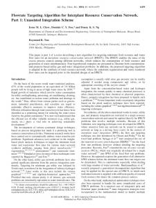
Numerical Results In this section, we present a numerical example of the RossbyHaurwitz wave test for the no hydrostatic Euler problem on a cubedsphere grid. We use the ne30np4 resolution (approximately 110 km) in the experiments. For horizontal grid spacing, ne indicates the number of quadrilateral elements in each direction for each face of the cube, and np is the number of Gauss-LegendreLobatto quadrature points. Throughout the numerical study in this section, numerical simulations are run for 3600(s) with a time step of ∆t. We will compare the numerical results of the semi-implicit time integration scheme ARK2 and the time-split explicit integration scheme SRK3. As the reference values of the test, we use the third-order explicit Runge-Kutta method, which will be abbreviated as RK3, with a very small time step ∆t=0.01(s). In general, RK3 is reasonably simple and robust. In these experiments of RK3, time steps smaller than 0.1(s) are used. If the time step is greater than 0.1(s), it is blow up. To apply the semi-implicit scheme, we have to solve the linear system using a numerical iterative solver. In this case, the generalized minimal residual method (GMRES) is applied without a preconditioned. The number of iterations in the numerical solver depends on the size of the matrix and its tolerance (tol). In this paper, we fixed tol=10−4. If we want to obtain a more accurate numerical solution by using the iterative solver, we can select a smaller tolerance than 10−4. The numerical results in ARK3, which are zonal wind u, meridional wind v, surface pressure ps and temperature θ at 850 hPa with ∆t=2.0(s), are presented in Figure 1. They are similar to the numerical results for RK3 (at ∆t=0.1(s)) and SRK3 (at ∆t=2.0(s)).
Figure 1: The numerical results u(top, left), v(top, right), ps(bottom, left) and θ(bottom, right) of ARK2 at 850 hPa are plotted with a final time T=3600(s) and ∆t=2.0(s).
J Appl Computat Math, an open access journal ISSN: 2168-9679
Volume 6 • Issue 4 • 1000369
Citation: Nam H, Choi SJ (2017) Implementation of a Semi-implicit Time Integration Scheme in Non-Hydrostatic Euler Equations. J Appl Computat Math 6: 369. doi: 10.4172/2168-9679.1000369
Page 5 of 7 The differences between the numerical results u, v, ps and θ for SRK3 and those for ARK2 at 850 hPa with ∆t=2.0(s) are presented in Figure 2. In figures, the L2-errors of different values for each variable are bounded by 10-5. SRK3 has faster computing times than ARK2 at the same time step because the linear system must be solved using the numerical iterative method in the semi-implicit scheme. In this paper, the semi-implicit scheme ARK2 is compared with the time-split Runge-Kutta explicit scheme SRK3 and we emphasize the accuracy of the semi-implicit scheme. We will show that ARK2 is more accurate than SRK3 for L2-error estimation. In L2-error estimation, we compute only the L2-error of the surface pressure ps in ARK2 and SRK3
for each time step, as in the following equation:
( ps )RK 3 − ( ps )h
L2
where (ps)RK3, as the reference numerical solution, is the value of the surface pressure from RK3 at ∆t=0.01(s). (ps)h, with h=SRK3 or ARK2, is the numerical solution of the surface pressure for each time step ∆t=0.2, 0.4, ··· , 2.0(s). Since SRK3 is the time-split scheme, each stage of the SRK3 is divided by a number of sub steps ns=2,4,8,16. ns is the ratio of the RK3 time step to the acoustic time step for the second and third RK3 sub steps. Figure 3 shows the L2-error of the surface pressure for each
Figure 2: The differences in the numerical results u(top, left), v(top, right), ps(bottom, left) and θ(bottom, right) for SRK3 and ARK2 at 850 hPa are plotted with a final time T=3600(s) and ∆t=2.0(s).
Figure 3: L2-error analysis of the surface pressure for each time step in SRK3 and ARK2. The L2-error estimations of SRK3 with the number of substeps ns=2,4,8,16, and ARK2 are plotted. The reference solution is the value of the surface pressure determined using RK3 at ∆t=0.01(s).
J Appl Computat Math, an open access journal ISSN: 2168-9679
Volume 6 • Issue 4 • 1000369
Citation: Nam H, Choi SJ (2017) Implementation of a Semi-implicit Time Integration Scheme in Non-Hydrostatic Euler Equations. J Appl Computat Math 6: 369. doi: 10.4172/2168-9679.1000369
Page 6 of 7
Figure 4: L2-error analysis of the surface pressure for each time step in ARK2. The L2-error estimations of only ARK2 are plotted. The reference solution is the value of the surface pressure determined using RK3 at ∆t=0.01(s). SRK3
ARK2
ARK3
Ps
4.81e-06
2.26e-09
2.31e-10
u
2.15e-06
8.90e-07
2.01e-07
v
1.85e-06
9.56e-07
2.82e-07
θ
6.95e-07
1.18e-10
8.33e-11
Table 1: At ∆t =1.0(s), L2-error analysis of numerical results ps, u, v and θin SRK3, ARK2, and ARK3 as the high order semi-implicit scheme. The reference value is obtained using RK3 at ∆t=0.01(s).
sub step ns. L -errors for the surface pressure are decreased when ns increases. In addition, since ARK2’s values are bounded by 10−8 and SRK3’s values are bounded by 10−4, we cannot compare the values directly in Figure 3. Thus, the L2-error of surface pressure of only ARK2 for each time step is presented in the right-hand side of Figure 4. From these results, for the same time step, we know that the L2-error of ARK2 is much smaller than that of SRK3. 2
We note that construction of the high-order ARK methods is complex and difficult. The third order ARK method with 4-stage, which we call ARK3, is only computed in this experiments. From Table 1, we observe that L2-errors for ARK2 and ARK3 are smaller than those for SRK3 and the values of ARK3 seem to be the smallest. However, since ARK3 has an additional stage, the total computing the time has to be increased. Thus, we know that ARK2 and ARK3 are more accurate than time split explicit scheme SRK3, while ARK2 and ARK3 are much slower than SRK3 in terms of computing time. If we consider the proper pre-conditioner in the iterative solver or transformation of the system with variable dependency, we can obtain a faster scheme. These are the topics of on-going research.
Conclusions In this paper, we implement the 3-stage additive Runge-Kutta method, which is a second-order semi-implicit time integration scheme, on the non-hydrostatic Euler problem with mass vertical coordinates. In this scheme, we use a larger time step than that used in the third-order RungeKutta explicit scheme, as the computing time in the semi-implicit scheme is long. This is done with the aim of solving the linear system with a numerical iteration scheme. Moreover, the time step of the semi-implicit scheme is larger than that of the original explicit Runge-Kutta scheme, but smaller than that of the timesplit Runge-Kutta explicit scheme. However, the numerical results J Appl Computat Math, an open access journal ISSN: 2168-9679
demonstrate that the s-stage additive Runge-Kutta semi-implicit time integration scheme is more accurate than other explicit schemes in the non-hydrostatic Euler problem. If we use a higher order additive Runge-Kutta semi-implicit scheme in this problem, more accurate numerical solutions are obtained. Acknowledgments This work has been carried out through the R&D project on the development of global numerical weather prediction systems of Korea Institute of Atmospheric Prediction Systems (KIAPS) funded by Korea Meteorological Administration (KMA).
References 1. Ascher U, Ruuth S, Spiteri R (1997) Implicit-explicit Runge-Kutta methods for time dependent partial differential equations. Applied Numerical Mathematics 25: 151-167. 2. Butcher J (2008) Numerical methods for ordinary differential equations. (2nd edn.), Wiley. 3. Choi SJ, Hong SY (2016) A global non-hydrostatic dynamical core using the spectral element method on a cubed-sphere grid. Asia-Pacific Journal of Atmospheric Sciences 52: 291-307. 4. Cullen M (1990) A test of a semi-implicit integration technique for a fully compressible nonhydrostatic model. Royal Meteorological Society 116: 12531258. 5. Davies T, Cullen M, Malcolm A, Mawson M, Staniforth A, et al. (2005)A new dynamical core for the Met office’s global and regional modelling of the atmosphere. Royal Meteorological Society 131: 1759-1782. 6. Durran D, Blossey P (2012) Implicit-explicit multistep methods for fast-waveslow-wave problems. Monthly Weather Review 140: 1307-1325. 7. Evans KJ, Taylor MA, Drake JB (2010) Accuracy analysis of a spectral element atmospheric model using a fully implicit solution framework. Monthly Weather Review 138: 3333-3341. 8. Giraldo FX (2005) Semi-implicit time-integrations for a scalable spectral element atmospheric model. Royal Meteorological Society 131: 2431-2454. 9. Giraldo FX, Kelly JF, Constantinescu EM (2012) Implicit-explicit formulations of a three dimensional nonhydrostatic unified model of the atmosphere (NUMA). SIAM: SIAM Journal on Scientific Computing 35: B1162-B1194. 10. Giraldo FX, Restelli M, Lauter M (2010) Semi-implicit formulations of the Navier-Stokes equations: application to nonhydrostatic atmospheric modeling. SIAM: SIAM Journal on Scientific Computing 32: 3394-3425. 11. Kennedy C, Carpenter M (2003) Additive Runge-Kutta schemes for convectiondiffusion reaction equations. Applied Numerical Mathematics 44: 139-181. 12. Klemp JB, Skamarock WC, Dudhia J (2007) Conservative split-explicit time
Volume 6 • Issue 4 • 1000369
Citation: Nam H, Choi SJ (2017) Implementation of a Semi-implicit Time Integration Scheme in Non-Hydrostatic Euler Equations. J Appl Computat Math 6: 369. doi: 10.4172/2168-9679.1000369
Page 7 of 7 integration methods for the compressible non-hydrostatic equations. Monthly Weather Review 135: 2897-2913.
model for weather research and forecasting applications. Journal of Computational Physics 227: 3465-3485.
13. Klemp JB, Wilhelmson RB (1978) Simulation of 3-dimensional convective storm dynamics. Journal of the Atmospheric Sciences 35: 1070-1096.
20. Skamarock WC, Klemp JB, Duda MG, Fowler LD, Park SH, et al (2012) A multiscale nonhydrostatic atmospheric model using centroidal voronoi tesselations and C-grid staggering. Monthly Weather Review 240: 3090-3105.
14. Kwizak M, Robert AJ (1971) A Semi-implicit scheme for grid point atmospheric models of the primitive equations. Monthly Weather Review 99: 32-36. 15. Laprise R (1992) The Euler equations of motion with hydrostatic pressure as an independent variable. Monthly Weather Review 120: 197-207. 16. Pareschi L, Russo G (2005) Implicit-explicit Runge-Kutta schemes and applications to hyperbolic systems with relaxation. Journal of Scientific Computing 25: 129-155. 17. Satoh M, Matsuno T, Tomita H, Miura H (2008) Nonhydrostatic icosahedral atmospheric model (NICAM) for global cloud resolving simulations. Journal of Computational Physics 227: 3486-3514. 18. Skamarock WC, Dudhia J, Gill DO, Barker DM, Duda MG, et al. (2008) A description of the advanced research WRF version 3. NCAR Tech. 19. Skamarock WC, Klemp JB (2008) A time-split nonhydrostatic atmospheric
J Appl Computat Math, an open access journal ISSN: 2168-9679
21. St-Cyr A, Neckels D (2009). A fully implicit Jacobian-free high-order discontinuous Galerkin mesoscale flow solver. Lecture Notes in Computer Science, 5545: 243-252. 22. Szmelter J, Smolarkiewicz P (2010) An edge-based unstructured mesh discretization in geophysical framework. Journal of Computational Physics 229: 4980-4995. 23. Thomas SJ, Loft RD (2005) The NCAR spectral element climate dynamical core: semi-implicit Eulerian formulation. Journal of Scientific Computing, 25: 307-322. 24. Ullrich P, Jablonowski C (2012) Operator-split Runge-Kutta-Rosenbrock methods for nonhydrostatic atmospheric models. Monthly Weather Review 140: 1257-1284. 25. Wicker LJ, Skamarock WC (2002) Time-splitting methods for elastic models using forward time schemes. Monthly Weather Review 130: 2088-2097.
Volume 6 • Issue 4 • 1000369