Implementation of a Speed Field Orientated Control of Three Phase

Implementation of a Speed Field Orientated Control of Three Phase AC Induction Motor using TMS320F240

Literature Number: BPRA076 Texas Instruments Europe March 1998

IMPORTANT NOTICE Texas Instruments and its subsidiaries (TI) reserve the right to make changes to their products or to discontinue any product or service without notice, and advise customers to obtain the latest version of relevant information to verify, before placing orders, that information being relied on is current and complete. All products are sold subject to the terms and conditions of sale supplied at the time of order acknowledgement, including those pertaining to warranty, patent infringement, and limitation of liability. TI warrants performance of its semiconductor products to the specifications applicable at the time of sale in accordance with TI’s standard warranty. Testing and other quality control techniques are utilized to the extent TI deems necessary to support this warranty. Specific testing of all parameters of each device is not necessarily performed, except those mandated by government requirements. CERTAIN APPLICATIONS USING SEMICONDUCTOR PRODUCTS MAY INVOLVE POTENTIAL RISKS OF DEATH, PERSONAL INJURY, OR SEVERE PROPERTY OR ENVIRONMENTAL DAMAGE (“CRITICAL APPLICATIONS”). TI SEMICONDUCTOR PRODUCTS ARE NOT DESIGNED, AUTHORIZED, OR WARRANTED TO BE SUITABLE FOR USE IN LIFE-SUPPORT DEVICES OR SYSTEMS OR OTHER CRITICAL APPLICATIONS. INCLUSION OF TI PRODUCTS IN SUCH APPLICATIONS IS UNDERSTOOD TO BE FULLY AT THE CUSTOMER’S RISK. In order to minimize risks associated with the customer’s applications, adequate design and operating safeguards must be provided by the customer to minimize inherent or procedural hazards. TI assumes no liability for applications assistance or customer product design. TI does not warrant or represent that any license, either express or implied, is granted under any patent right, copyright, mask work right, or other intellectual property right of TI covering or relating to any combination, machine, or process in which such semiconductor products or services might be or are used. TI’s publication of information regarding any third party’s products or services does not constitute TI’s approval, warranty or endorsement thereof.

Copyright  1998, Texas Instruments Incorporated

Contents

Contents 1. Introduction ..............................................................................................................1 2. The Field Orientated Controlled AC Induction Drive ................................................2 2.1 The AC induction motor.................................................................................2 2.2 The control hardware ....................................................................................3 2.3 The Power Electronics Hardware..................................................................3 2.4 Complete Field Orientated Speed Control Structure Presentation................4 3. Field Orientated Speed Controlled AC Induction Drive Software Implementation ...6 3.1 Software Organization...................................................................................6 3.1.1 DSP Controller Setup...................................................................7 3.1.2 Software Variables.......................................................................7 3.2 Base values and PU model ...........................................................................8 3.3 Magnetizing current considerations...............................................................9 3.4 Numerical considerations ............................................................................10 3.4.1 The numeric format determination .............................................10 3.5 Current Sensing and Scaling.......................................................................12 3.6 Speed Sensing and Scaling ........................................................................15 3.7 The PI regulator ..........................................................................................17 3.8 Clarke and Park transformation...................................................................18 3.8.1 The (a,b)->(α,β) projection (Clarke transformation) ...................19 3.8.2 The (α,β)->(d,q) projection (Park transformation) ......................20 3.9 The current model .......................................................................................21 3.9.1 Theoretical background .............................................................21 3.9.2 Numerical consideration ............................................................22 3.9.3 Code and experimental results ..................................................23 3.10 Generation of sine and cosine values .......................................................25 3.11 The Field Weakening ................................................................................26 3.11.1 Field Weakening Principles......................................................26 3.11.2 Field Weakening Constraints ...................................................27 3.11.3 TMS320F240 Field Weakening Implementation ......................28 3.12 The Space Vector Modulation ...................................................................31 3.13 Experimental Results ................................................................................34 3.14 The control algorithm flow chart ................................................................37 4. User Interface.........................................................................................................39 5. Conclusion .............................................................................................................39 References.................................................................................................................40 Appendix A - TMS320F240 FOC Software ................................................................41 Appendix B - Linker File .............................................................................................64


iii

Contents

Appendix C - Sine Look-up table ............................................................................... 65 Appendix D - User Interface Software ....................................................................... 69

iv

Literature Number: BPRA076

Contents

List of Figures Figure 1: Top View of the TMS320F240 Evaluation Module .............................................3 Figure 2: Complete AC Induction Drive Dedicated FOC Structure....................................5 Figure 3: General Software Flowchart...............................................................................6 Figure 4: FOC Software Initialization and Operating System ............................................7 Figure 5: Steady State Phase Electrical Model .................................................................9 Figure 6: 4.12 Format Correspondence Diagram ............................................................10 Figure 7: 1) left shift & store high accumulator, 2) right shift & store low accumulator ....11 Figure 8: Current Sensing and Scaling Block Diagram ...................................................12 Figure 9: Current Sensing Interface Block Diagram ........................................................12 Figure 10: Sensed Current Values before Scaling ..........................................................13 Figure 11: 8.8 Numerical Format Correspondence Diagram...........................................14 Figure 12: Speed feedback obtaining block scheme.......................................................15 Figure 13: Speed Feedback Computation Flowchart ......................................................16 Figure 14: AC Induction Drive Phase Currents................................................................19 Figure 15: Output of the Clarke Transformation Module .................................................20 Figure 16: Link between Rotor Flux Position and its Numerical Representation .............22 Figure 17: Input and output for the current model block..................................................23 Figure 18: Rotor Flux Position, Flux and Torque Components........................................24 Figure 19: Sinθcm Calculation using the Sine Look-up Table ...........................................25 Figure 20: Field weakening Real Operation ....................................................................26 Figure 21: Maximum and Nominal Torque vs Speed ......................................................27 Figure 22: Field Weakening Voltage Constraints ............................................................28 Figure 23: Field Weakening Block Diagram ....................................................................28 Figure 24: Matlab Interpolation Results and Numerical Implementation Result ..............30 Figure 25: Experimental Torque & Power Charact. in the Extended Speed Range ........30 Figure 26: Table Assigning the Right Duty Cycle to the Right Motor Phase ...................33 Figure 27: Sector 3 PWM Patterns and Duty Cycles.......................................................34 Figure 28: Steady State Operation under Nominal Conditions........................................35 Figure 29: Transient Operation under Nominal Torque / Torque Limitation set to 0.8 ....35 Figure 30: Transient Operation under Nominal Torque / Torque Limit. set to 1.2 ...........36 Figure 31: Transient Operation in the Extend. Speed Range / Torque Limit. set to 1 .....36 Figure 32: Speed Reversion from -1000rpm to 1000rpm under nominal load.................37 Figure 33: FOC Implementation Flowchart......................................................................38 Figure 34: Communication Program. Screen picture.......................................................39


v

Introduction

Implementation of a Sensorless Speed Controlled Brushless DC Drive using the TMS320F240 ABSTRACT

Since the integration of high computationnal DSP power with all necessary motor control peripherals into a single chip, TMS320F240, it has become possible to design and implement a highly efficient and accurate AC induction drive control. The AC induction drive presented here is based on document [6] and on a dedicated and exhaustive study of this DSP solution. Both the theoretical and practical characteristics of this drive implementation allow the reader to quickly gain an understanding of the Field Orientated Control of an induction motor. As such, the reader might not only gain a short time to market solution, but also a speed adjustable, reliable and highly effective induction drive.

1. Introduction For many years the asynchronous drive has been preferred for a variety of industrial applications because of its robust nature and simplicity of control. Until a few years ago, the asynchronous motor could either be plugged directly into the network or controlled by means of the well-known scalar V/f method. When designing a variable speed drive, both methods present serious drawbacks in terms of the drive efficiency, the drive reliability and EMI troubles. With the first method, even simple speed variation is impossible and its system integration highly dependent on the motor design (starting torque vs maximum torque, torque vs inertia, number of pole pairs). The second solution is able to provide a speed variation but does not handle real time control as the implemented is valid only in steady stage. This leads to over-currents and over-heating, which necessitate a drive which is then oversized and no longer cost effective. It is the real time-processing properties of silicon, such as the TMS320F240 DSP controller, and the accurate asynchronous motor model that have resulted in the development of a highly reliable drive with highly accurate and variable speed controls. Application of The Field Orientated Control to the AC induction drive results in the instant control of a high performance drive (short response time with neither the motor nor the power component oversized). The ability to achieve such control renders the asynchronous drive a highly advantageous system for both home appliances and for industrial or automotive applications. Key advantages are the robust nature of the drive, its reliability and efficiency, the cost effectiveness of both the motor and the drive, the high torque at zero speed, the speed variation capacity, the extended speed range, the direct torque and flux control and the excellent dynamic behaviour. In this document we will look not only at the complete integration of the software, but also at the theoretical and practical aspects of the application. By the end of this report the reader will have gained an understanding of each of the developmental steps and will be able to apply this asynchronous drive solution to his own system.


1

The Field Orientated Controlled AC Induction Drive

The first section deals with the presentation of the field orientated controlled AC induction drive; it explains the AC induction motor, the control hardware, the power electronics hardware as well as the complete FOC structure. The second section deals with the implementation of TMS320F240 drive speed control. Here, the details of how and why the software is organized, the Per Unit model, the numerical consideration, the current and speed sensing and scaling, the regulators, the system transformations, the current model, the field weakening and the space vector modulation are fully explained step by step. Results of intermediate experiments illustrate the presentations in each block. At the end of this document flowcharts have been incorporated to explain the operating system. The final experiment results demonstrate the dynamic behaviour and effectiveness of the drive.

2. The Field Orientated Controlled AC Induction Drive This chapter presents each component of the AC induction drive. The different subchapters cover the motor parameters and the implemented control structure, including both the control and the power hardware 2.1 The AC induction motor The AC induction machine used in this explanation is a single cage three phase Yconnected motor. The rated value and the parameters of this motor are as follows: Rated power Pn=500W Rated voltage Vn=127V rms (phase) Rated current In=2.9A rms Rated speed 1500rpm Pole pairs 2 Slip 0.066 Pnom 500 Rated torque M nom = = = 3.41Nm ω nom  2π ×1400     60  Stator resistance (RS) Magnetizing inductance (LH) Stator leakage inductance (LσS) Stator inductance (LS=LσS+LH) Rotor leakage inductance (LσR) Rotor inductance (LR=LσR+LH) Rotor resistance (RR) Rotor inertia

4.495Ω 149mH 16mH 165mH 13mH 162mH 5.365Ω -3 2 0.95*10 Kgm

An embedded incremental encoder is also provided with this motor. This is capable of 1000 pulses per revolution and is used in this application to obtain the rotor mechanical speed feedback.

2



2.2 The control hardware The control hardware can be either the TMS320F240 Evaluation Module introduced by Texas Instruments or the MCK240 developed by Portescap/Technosoft. In this application the second board can be plugged directly on to the power electronics board. The two boards contain a DSP controller TMS320F240 and its oscillator, a JTAG, and an RS232 link with the necessary output connectors. The figure below depicts the EVM board.

Figure 1: Top View of the TMS320F240 Evaluation Module The EVM board provides access to any signal from the DSP Controller and contains test LED’s and Digital to Analog Converters. These characteristics are particularly interesting during the developmental stage. 2.3 The Power Electronics Hardware The power hardware used to implement and test this AC induction drive can support an input voltage of 220V and a maximum current of 10A. It is based on six power IGBT (IRGPC40F) driven by the DSP Controller via the integrated driver IR2130. The power and the control parts are insulated by means of opto-couplers. The phase current sensing is performed via two current voltage transducers supplied with +/-15V. Their maximum input current is 10A, which is converted into a 2.5V output voltage. Furthermore, this powered electronics board supports bus voltage measurement, control LED’s and input current filter. All the power device securities are wired (Shutdown, Fault, Clearfault, Itrip, reverse battery diode, varistor peak current protection).


3


2.4 Complete Field Orientated Speed Control Structure Presentation The control algorithm implemented in this application report is a rotor flux orientated control strategy, based on the Field Orientated Control structure presented in [6]. Given the position of the rotor flux and two phase currents, this generic algorithm operates the instantaneous direct torque and flux controls by means of coordinate transformations and PI regulators, thereby achieving a really accurate and efficient motor control. The generic FOC structure needs to be augmented with two modules in order to address the asynchronous drive specificity. With the asynchronous drive, the mechanical rotor angular speed is not, by definition, equal to the rotor flux angular speed. This implies that the necessary rotor flux position can not be detected directly by the mechanical position sensor provided with the asynchronous motor used in this application. The Current Model block must be added to the generic structure in the block diagram. This current model [1][3][5] takes as input both iSq and iSd current as well as the rotor mechanical speed and gives the rotor flux position as output. A complete description and the software implementation for the necessary equations are given in a subsequent chapter. The speed control of the AC induction drive is often split into two ranges: the low speed range, where the motor speed is below the nominal speed, and the high speed range, where the motor speed is higher than the nominal speed. Above the nominal speed the effective back electromotive force (which depends on both the motor speed and on the rotor flux) is high enough, given the DC bus voltage limitation, to limit the current in the winding. As such, this limits both the torque production and the drive efficiency (due to problems with magnetic saturation and heat dissipation). Where the rotor flux has been maintained at its nominal value during the low speed operation so as to achieve the highest mutual torque production, it must be reduced in the high speed operation in order to avoid magnetic saturation and the generation of too high back electromotive force. Reducing the rotor flux in this way extends the high efficiency operating range of the drive. This functionality is integrated into the Field Weakening module. A complete explanation and outline of the correct software implementation are given in a later chapter.

4



These two induction motor control dedicated modules are added to the basic FOC structure. This results in the following complete FOC AC induction drive structure:

nref

PI

iSqref

-

PI

vSqref

Park -1 t.

d,q

iSdref Field Weakening

PI

vSdref

α,β

VDC

vSαref vSβref

SV PWM

3-phase Inverter

θcm current model

iSq iSd

d,q α,β Park t.

iSα iSβ

α,β

a,b,c

ia ib

Clarke t.

Induction

n

motor

Figure 2: Complete AC Induction Drive Dedicated FOC Structure Two phase currents feed the Clarke transformation module. These projection outputs are indicated iSα and iSβ. These two components of the current provide the input of the Park transformation that gives the current in the d,q rotating reference frame. The iSd and iSq components are compared to the references iSdref (the flux reference) and iSqref (the torque reference). The torque command iSqref corresponds to the output of the speed regulator. The flux command iSdref is the output of the field weakening function that indicates the right rotor flux command for every speed reference. The current regulator outputs are vSdref and vSqref; they are applied to the inverse Park transformation. The output of this projection are vSαref and vSβref, the components of the stator vector voltage in the α,β orthogonal reference frame. These are the input of the Space Vector PWM. The outputs of this block are the signals that drive the inverter. Note that both Park and inverse Park transformations require the rotor to be in flux position which is given by the current model block. This block needs the rotor resistance as a parameter. Accurate knowledge and representation of the rotor resistance is essential to achieve the highest possible efficiency from the control structure.


5

Field Orientated Speed Controlled AC Induction Drive Software Implementation

3. Field Orientated Speed Controlled AC Induction Drive Software Implementation This chapter deals with the practical aspects of the drive implementation. It describes the software organization, the utilization of different variables and the handling of the DSP Controller resource. In the second part the control structure for the per unit model is presented. This explanation allows the reader to instantly adapt the given software to match the parameters of his drive. As numerical considerations have been made in order to address the problems inherent within fixed-point calculation, this software can be used with a wide range of drive parameters and regulator coefficients. 3.1 Software Organization This software is based on two modules: the initialization module and the run module. The former is performed only once at the beginning. The second module is based on a waiting loop interrupted by the PWM underflow. When the interrupt flag is set, this is acknowledged and the corresponding Interrupt Service Routine (ISR) is served. The complete FOC algorithm is computed within the PWM ISR and thus runs at the same frequency as the chopping frequency. The waiting loop can be easily replaced by a user interface. Presentation of the interface is beyond the scope of this report, but is useful to fit the control code and to monitor the control variables. An overview of the software is given in the flow chart below: S ta rt

H ard w are I n itia liz a ti o n S W V a r ia b l e s I n itia liz a ti o n

W a itin g L oop PW M IS R

Figure 3: General Software Flowchart The DSP Controller Full Compare Unit is used to generate the necessary pulsed signals to the power electronics board. It is programmed to generate symmetrical complementary PWM signals at a frequency of 10kHz, with TIMER1 as the time base and with the DEADBAND unit disabled. The sampling period (T) of 100 µs can be established by setting the timer period T1PER to 1000 (PWMPRD=1000).

6



The following figure illustrates the time diagram for the initialization and the operating system. PWM Underflow Interrupt Sampling Period T=100µs=2*PWMPRD

T1CNT

PWMPRD=1000*50ns=50µs Initialization

τ algorithm

Waiting Time

τ algorithm

Software Start

Figure 4: FOC Software Initialization and Operating System

3.1.1 DSP Controller Setup This section is dedicated to the handling of the different DSP Controller resources (Core and peripheral settings). First of all, the PLL unit is set so that the CPUCLK runs at 20MHz based on the 10Mhz quartz provided on the EVM board. For the developmental stage it is necessary to disable the watchdog unit: first set the Vccp pin voltage to five volts utilising the EVM jumper JP5 and then set the two watchdog dedicated registers to inactive. Finally, correctly set the core and EV mask registers to enable the PWM underflow to interrupt serving.

3.1.2 Software Variables The following lines show the different variables used in this control software and in the equations and schemes presented here. ia, ib, ic phase current stator current (α,β) components iSα, iSβ iSd, iSq stator current flux & torque comp. iSdref, iSqref flux and torque command Teta_cm or θcm rotor flux position fs rotor flux speed i_mR, imR magnetizing current vSdref, vSqref (d,q) components of the stator voltage vSαref, vSβref (α,β) components of the stator voltage (input of the SVPWM) vDC DC bus voltage vDCinvT constant using in the SVPWM vref1, vref2, vref3 voltage reference used for SV sector determination sector sector variable used in SVPWM t1, t2 time vector application in SVPWM taon, tbon, tcon PWM commutation instant


7


X, Y, Z n, nref iSqrefmin, iSqrefmax vmin,vmax Ki, Kpi, Kcor Kin, Kpin, Kcorn xid, xiq, xin epid, epiq, epin K r , K t, K p 3, p2, p1, p0 Kspeed, SPEEDSTEP speedstep encincr, speedtmp Kcurrent sinθcm, sinTeta_cm, cosθcm, cosTeta_cm

SVPWM variables speed and speed reference speed regulator output limitation d,q current regulator output limitation current regulator parameters speed regulator parameters regulator integral components d,q-axis, speed regulator errors current model parameters field weakening polynomial coeff 4.12 speed formatting constant speed loop period speed loop counter encoder pulses storing variable occurred pulses in SPEEDSTEP 4.12 current formatting constant sine and cosine of the rotor flux position

3.2 Base values and PU model Since the TMS320F240 is a fixed point DSP, a per unit (pu) model of the motor has been used. In this model all quantities refer to base values. The base values are determined from the nominal values by using the following equations, where In, Vn , fn are respectively the phase nominal current, the phase to neutral nominal voltage and the nominal frequency in a star-connected induction motor Ib = 2I n V

b

ω Ψ

=

2V

n

b

= 2π f

n

b

=

V

b

ω

b

and where Ib, Vb are the maximum values of the phase nominal current and voltage; ωb is the electrical nominal rotor flux speed; Ψb is the base flux. The base values of the motor used in this asynchronous drive are stated below. I b = 2 I n = 2 ⋅ 2 .9 = 4 .1 A V b=

2V n =

2 ⋅ 127 ≅ 180 V

ω b = 2π f n = 2π ⋅ 50 = 314 . 15 Ψb =

8


rad sec

Vb 180 = = 0 . 571 Wb ωb 314 . 15


The real quantities are implemented in to the control thanks to the pu quantities, which are defined as follows: I i= Ib v=

V Vb

ψ=

Ψ Ψb

n=

electrical rotor speed pole pairs * mechanical rotor speed = ωb ωb

fS =

rotor flux speed ωb

Where LYψQI6 are respectively pu current, voltage, flux, electrical rotor speed and rotor flux speed. This model can be followed to ensure the easy implementation of the control algorithm into a fixed point DSP. 3.3 Magnetizing current considerations In the classic speed range (where speed is lower or equal to the nominal speed) the FOC structure requires the magnetizing current as input. Given the following motor equivalent circuit, valid only in stationary steady state, the magnetizing current might be a priori calculated.

IS

RS

LσS

RR

LσR Itorque

ImR V

LH

1− s  RR    s 

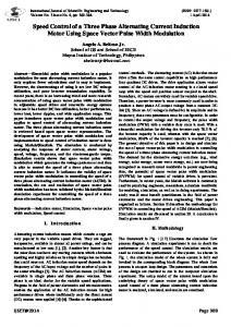
Figure 5: Steady State Phase Electrical Model Assuming that the motor is running at nominal speed without any load (in other words that slip is equal to zero) and knowing the paramaters of the motor, then the magnetizing current is simply equal to the nominal phase voltage (in this case 127V rms) divided by the equivalent impedance. A useful tip is to know that the magnetizing current is usually between 40% and 60% of the nominal current.


9


3.4 Numerical considerations The PU model has been developed so that the software representation of speed current and flux is equal to one when the drive has reached its nominal speed under nominal load and magnetizing current. Bearing in mind that during the transient the current might reach higher values than the nominal current (Ib) in order to achieve a short response time, and assuming that the motor speed range might be extended above the nominal speed (ωb), then every per unit value might be greater than one. This fact forces the implementation to foresee these situations and thereby determine the most suitable numerical format.

3.4.1 The numeric format determination The numeric format used in the major part of this application is such that 4 bits are dedicated to the integer part and 12 bits are dedicated to the fractional part. This numeric format is denoted by 4.12 f. The resolution for this format is: 1 = 0.00024414 212 With the sign extension mode set, the link between the real quantity and its 4.12 representation is illustrated by the following chart:

32767

-8 24.4e-5 7.99975586

-32768

Figure 6: 4.12 Format Correspondence Diagram The reason for selecting this particular format is that the drive control quantities are (for the most part) not greater than four times their nominal values (in other words, not greater than four when the pu model is considered). Where this is not the case,a different format will be chosen. The selection of a demonstration range of [-8;8] ensures that the software values can handle each drive control quantity, not only during steady state operation but also during transient operation. The next two paragraphs outline some of the numerical considerations and some operations with a generic x.y format in order to explain the different formats that can be found in this application report.

10



The x.y numeric format uses x bits for the integer part and y bits for the fractional part. The resolution is 2 − y ; if z is the pu value to implement, then its software value is z ⋅ 2 y in x.y format. Care must be taken when performing operations with a generic x.y format. Adding two x.y-formatted numbers may result in numerical representation overflow. To avoid this kind of problem, one possible solution is to perform the addition in the high side of the Accumulator and to set the saturation bit. Another option is to assume that the result will not be out of the maximum range. This second solution can be used in this implementation if we know that the control quantities do not exceed half of the maximum value in the 4.12 format. The result can still be represented in the 4.12 format and directly considered as 4.12 format, thereby allowing for a higher level of precision. As far as the multiplication is concerned, the result (in the 32-bit Accumulator) must either be shifted x position to the left and the most significant word stored, or be shifted y position to the right with the last significant word being stored. The stored result is in x.y format. The figure below shows two x.y-formatted 16-bit variables, that will be multiplied by one another. The result of this multiplication in x.y format is represented in gray in the 32-bit Accumulator. Both solutions are depicted below. x x y y MSB

LSB

MSB

LSB

* x

y

MSB

LSB

x

y

1 x

y

2 high word

low word

Figure 7: 1) left shift & store high accumulator, 2) right shift & store low accumulator Note that in this application there are also constants that can not be represented by the 4.12 format. Operations requiring different formats follow exactly the same process as that explained above.


11


3.5 Current Sensing and Scaling The FOC structure requires two phase currents as input. In this application currentvoltage transducers (LEM type) sense these two currents. The current sensor output therefore needs to be rearranged and scaled so that it can be used by the control software as 4.12 format values. The complete process of acquiring the current is depicted in the figure below: I

ix Kcurrent

511 : -512

range adjustement

1023 : 0

10-bit A/D

interface

LEM

x=a,b

TMS320F240

Figure 8: Current Sensing and Scaling Block Diagram In this application the LEM output signal can be either positive or negative. This signal must therefore be translated by the analogue interface into a range of (0;5V) in order to allow the single voltage ADC module to read both positive and negative values. The block diagram below shows the different steps of the implemented current sensing: 2.5V analog Offset

LEM OA Output Voltage

ADC Input Volts 5

LEM Output Voltage

Volts Imax

2.5

2.5

0

0

-2.5

Volts Imax

-Imax

Figure 9: Current Sensing Interface Block Diagram Note that Imax represents the maximum measurable current, which is not necessarily equal to the maximum phase current. This information is useful at the point where current scaling becomes necessary. The ADC input voltage is now converted into a ten bits digital value. The 2.5V analogue offset is digitally subtracted from the conversion result, thereby giving a signed integer value of the sensed current.

12



The result of this process is represented below: Numerical Value before Scaling 511 -Imax

0

Sensed Current Imax -512

Figure 10: Sensed Current Values before Scaling Like every other quantity in this application, the sensed phase currents must now be expressed with the pu model and then be converted into the 4.12 format. Notice that the pu representation of the current is defined as the ratio between the measured current and the base current and that the maximum current handled by the hardware is represented by 512. The pu current conversion into the 4.12 format is achieved by multiplying the sensed current by the following constant: 4096 K current = 512 ⋅ I b ( ) I max In one single calculation, this constant performs not only the pu modeling but also the numerical conversion into 4.12 format. When nominal current flows in a motor running at nominal speed, the current sensing and scaling block output is 1000h (equivalent to 1pu). The reader may change the numerical format by simply amending the numerator value and may adapt this constant to its own current sensing range by simply recalculating KcurrenW with its own Imax value. In this application the maximum measurable current is Imax=10A . The constant value is: 4096 K current = = 19.51 ⇔ 1383h 8.8 f 512 ⋅ 4.1 ( ) 10 Note that Kcurrent is outside the 4.12 format range. The most appropriate format to accommodate this constant is the 8.8 format, which has a resolution of: 1 0.00390625 = 8 2 and the following correspondence (Figure 11):


13


32767

-128 39.06e-4 127.996

-32768

Figure 11: 8.8 Numerical Format Correspondence Diagram The two phase currents are sampled simultaneously by means of the DSP Controller by using one channel of each ADC module per current. In this application channel 1 (ADCIN0) and channel 9 (ADCIN8) are used to sample the phase currents. Below is the code that waits for the LEM output to be converted and then transforms the conversion result into a 4.12 representation of one phase current. *********************************************************** * Current sampling - AD conversions * N.B. we will have to take only 10 bit (LSB) *********************************************************** ldp #DP_PF1 splk #1801h,ADC_CNTL1 ;ia and ib conversion start ;ADCIN0 selected for ia A/D1 ;ADCIN8 selected for ib A/D2 conversion bit ADC_CNTL1,8 bcnd conversion,tc ;wait approximatly 6us lacc ADC_FIFO1,10 ;10.6 format ldp #ctrl_n ;control variable page sach tmp lacl tmp and #3ffh sub #512 ;then we have to subtract the offset (2.5V) to have ;positive and negative values of the sampled current sacl tmp spm 3 ;PM=11, 6 right shift after multiplication lt tmp mpy Kcurrent pac ; sfr sfr sacl ia ;PM=11, +2 sfr= 8 right shift spm 0 sub #112 ;then we subtract a DC offset ;(that should be zero, but it ;isn't) sacl ia ;sampled current ia, 4.12 format spm 0 ;PM=00 *********************************************************** * END Current sampling - AD conversions ***********************************************************

14



For the minimum and maximum values of the phase current, the following table shows the contents of the ADCFIFO1 register: ADC module Input Voltage 0V 5V

Related current Imin Imax

ADCFIFO1 hexa. Value 0000h FFC0h

ADCFIFO1 binary value 0000 0000 0000 0000b 1111 1111 1100 0000b

This current sensing and scaling module requires 45 words of ROM, 4 words of RAM and 1.98MIPS (this includes the conversion time). 3.6 Speed Sensing and Scaling In this AC induction drive a 1000 pulse incremental encoder produces the rotor speed. The two sensor output channels (A and B) are wired directly to the QEP unit of the DSP Controller TMS320F240, which counts both edges of the pulses. The software speed resolution is thus based on 4000 increments per revolution. The QEP assigned timer counts the number of pulses, as recorded by the timer counter register (T3CNT). At each sampling period this value is stored in a variable named encincr. As the mechanical time constant is much lower than the electrical one, the speed regulation loop frequency might be lower than the current loop frequency. The speed regulation loop frequency is achieved in this application by means of a software counter. This counter takes as input clock the PWM interrupt. Its period is the software variable called SPEEDSTEP. The counter variable is named speedstep. When speedstep is equal to SPEEDSTEP, the number of counted pulses is stored in another variable called speedtmp and thus the speed can be calculated. The following scheme depicts the structure of the speed feedback generation: QEP1 (A)

n

Kspeed

speedtmp

if

encincr

speedstep=SPEEDSTEP

counter

encoder

(QEP circuit) ∗4

QEP2 (B)

TMS320F240

Figure 12: Speed feedback obtaining block scheme

Assuming that np is the number of encoder pulses in one SPEEDSTEP period when the motor turns at the nominal speed, a software constant Kspeed should be chosen as follows: 01000h = Kspeed ⋅ n p to let the speed feedback be transformed into a 4.12 format, that can be used with the control software. In this application the nominal speed is 1500 rpm, SPEEDSTEP is set to 30 and then np can be calculated as follows: 1500 ⋅ 4000 np = ⋅ SPEEDSTEP ⋅ T = 300 60 and hence Kspeed is given by:


15


Kspeed =

4096 = 13.653 ⇔ 0da 7h 300

8.8f

Note that Kspeed is out of the 4.12 format range. The most appropriate format to handle this constant is the 8.8 format. The speed feedback in 4.12 format is then obtained from the encoder by multiplying speedtemp by Kspeed . The flow chart and the code for speed sensing is presented below:

T3CNT Read Value in encincr

speedstep=speedstep-1

speedstep=0?

YES

NO

n=Kspeed*speedtemp

speedstep=SPEEDSTEP

speedtemp= speedtemp+encincr

Figure 13: Speed Feedback Computation Flowchart ************************************** * Measured speed and control ************************************** *** encoder pulses reading ldp #DP_EV lacc T3CNT ;we read the encoder pulses splk #0000h,T3CNT ldp #ctrl_n ;control variable page sacl encincr *** END Encoder pulses reading ******************************************************* * Calculate speed and update reference speed variables ******************************************************* lacc speedstep ;are we in speed control loop ;(SPEEDSTEP times current control loop) sub #1 sacl speedstep bcnd nocalc,GT ;if we aren't, skip speed calculation

16



********************************************** * Speed calculation from encoder pulses ********************************************** spm 3 ;PM=11, 6 right shift after multiplication lt speedtmp ;multiply encoder pulses by Kspeed ;(8.8 format constant) ;to have the value of speed mpy #Kspeed pac sfr sfr ;PM=11, +2 sfr= 8 right shift sacl n lacc #0 ;zero speedtmp for next ;calculation sacl speedtmp lacc #SPEEDSTEP ;restore speedstep to the value ;SPEEDSTEP sacl speedstep ;for next speed control loop spm 0 ;PM=00, no shift after multiplication ********************************************** * END Speed calculation from encoder pulses **********************************************

This speed sensing and scaling module requires 28 words of ROM, 4 words of RAM and 0.244 MIPS (which includes the speed reference acquisition time).

3.7 The PI regulator The PI (Proportional-Integral) regulators are implemented with output saturation and with integral component correction. Please refer to report [6] for any further PI structure information. The constants Kpi, Ki, Kcor (proportional, integral and integral correction components) are selected depending on the sampling period and on the motor parameters. In this application ( T=100µs sampling time) the current loop constants are: Ki = 0.0625 ⇔ 0100h K pi = 1 ⇔ 01000h K cor =

Ki = 0.0625 ⇔ 0100h K pi

And the speed loop constants are: K in = 0.0129 ⇔ 0035h K pin = 4.510 ⇔ 0482 Bh K corn =

K in = 0.00268 ⇔ 0 Bh K pin

Note that all constants are in 4.12 format and the integral correction component is calculated by using the following formula: K K cor = i K pi


17


As speed and current regulator have exactly the same software structure, only the speed regulator code is given below. ***************************************************** * Speed regulator with integral component correction ***************************************************** lacc n_ref sub n sacl epin ;epin=n_ref-n, 4.12 format lacc xin,12 lt epin mpy Kpin apac sach upi,4 ;upi=xin+epin*Kpin, 4.12 format ;here we start to saturate bit upi,0 bcnd upimagzeros,NTC ;If value >0 we branch lacc #Isqrefmin ;negative saturation sub upi bcnd neg_sat,GT ;if upiISqrefmax then branch to saturate upi ;value of upi valid limiters #Isqrefmax

;set acc to +ve saturated value

sacl sub sacl

iSqref upi elpi

;Store the acc as reference value

lt mpy pac lt mpy apac add sach

elpi Kcorn

;if there is no saturation elpi=0

limiters ;elpi=iSqref-upi, 4.12 format

epin Kin xin,12 xin,4

;xin=xin+epin*Kin+elpi*Kcorn, 4.12 format

*********************************************************** * END Speed regulator with integral component correction ***********************************************************

where iSqrefmin and iSqrefmax are the speed regulator limitations. Each PI regulator module requires 44 words of ROM, 10 words of RAM and 0.44 MIPS. 3.8 Clarke and Park transformation In the next two paragraphs, the TMS320F240 code and experimental results relevant to both the Clarke and Park transformation will be presented. The corresponding theoretical background explanations have already been handled in [6].

18



3.8.1 The (a,b)->(α,β) projection (Clarke transformation) In the following code the considered constant and variables are implemented in 4.12 format. ********************************************* * Clarke transformation * (a,b) -> (alfa,beta) * iSalfa = ia * iSbeta = (2 * ib + ia) / sqrt(3) ********************************************* lacc ia sacl iSalfa ;iSalfa 4.12 format add ib neg sacl ic lacc add sacl lt mpy

ib,1 ia tmp tmp #SQRT3inv

;iSbeta = (2 * ib + ia) / sqrt(3)

;SQRT3inv = (1 / sqrt(3)) = 093dh ;4.12 format = 0.577350269

pac sach iSbeta,4 ;iSbeta 4.12 format ********************************** * END Clarke transformation **********************************

where SQRT3inv is the following constant: 1 SQRT 3inv = = 0.577 ⇔ 093dh 3

4.12 f

Scope pictures of the a,b,c currents (input of the Clarke module) and the α,β currents (output of this module) are presented below.

Figure 14: AC Induction Drive Phase Currents This balanced three-phase system is shown below when transformed into the (α,β) orthogonal frame:


19


Figure 15: Output of the Clarke Transformation Module The upper visual depicts the two coordinates Clarke transformation system. The lower visual is an X-Y representation of the transformation output where α is the X input and β is the Y input. This illustrates the resulting orthogonal system. This Clarke transformation module requires 12 words of ROM, 6 words of RAM and 0.24 MIPS.

3.8.2 The (α α,β β)->(d,q) projection (Park transformation) In the following code the constant and variables under consideration are implemented in 4.12 format. The quantity Teta_cm represents the rotor flux position calculated by the current model. *********************************************** * Park transformation * (alfa, beta)->(d,q) * iSd=iSalfa*cos(Teta_cm)+iSbeta*sin(Teta_cm) * iSq=-iSalfa*sin(Teta_cm)+iSbeta*cos(Teta_cm) *********************************************** lt iSbeta mpy sinTeta_cm lta iSalfa mpy cosTeta_cm mpya sinTeta_cm sach iSd,4 ;iSd 4.12 format

20



lacc #0 lt iSbeta mpys cosTeta_cm apac sach iSq,4 ;iSq 4.12 format ********************************** * END Park transformation **********************************

SinTeta_cm and cosTeta_cm indicate respectively the Teta_cm sine and cosine values. The modalities required to determine these values are explained later in this document. This Park transformation module requires 12 words of ROM, 6 words of RAM and 0.24 MIPS.

3.9 The current model This chapter represents the core module of the Field Orientated Controlled AC induction drive. This module takes as input iSd , iSq plus the rotor electrical speed. In addition to the two essential equations, the numerical considerations, code and experimental results will also be discussed.

3.9.1 Theoretical background The current model [1][2][3][5] consists of implementing the following two equations of the motor in d,q reference frame: di idS = TR mR + i mR dt i qS 1 dθ fS = = n+ ω b dt TR imRω b where θ is the rotor flux position, imR the magnetizing current, and where L TR = R RR is the rotor time constant. Knowledge of this constant is critical to the correct functioning of the current model as it is this system that outputs the rotor flux speed that will be integrated to get the rotor flux position. Assuming that i qSk +1 ≈ i qSk the above equations can be discretized as follows: imRk +1 = imRk +

T (idS k − i mRk ) TR

f S k +1 = nk +1 +

1 iqS k TRω b imRk +1

Implementation of the software for these equations is handled in the following chapters.


21


3.9.2 Numerical consideration Let the two above equation constants

T 1 be renamed respectively Kt and and TR TR ω b

KR . In this application their values are:

100 ⋅ 10 −6 T = = 3.3117 ⋅ 10 − 3 ⇔ 0eh 4.12 f −3 TR 30195 . ⋅ 10 1 1 = = 105.42 ⋅ 10 − 3 ⇔ 01b0h 4.12 f Kt = TR ω b 30195 . ⋅ 10 − 3 ⋅ 314.15

KR =

Once the rotor flux speed (fS) has been calculated, the necessary rotor flux position (θcm) is computed by the integration formula: θ cmk +1 = θ cmk + ω b f S k T As the rotor flux position range is [0;2π], 16 bit integer values have been used to achieve the maximum resolution. The following chart demonstrates the relationship between the flux position and its numerical representation: 65535

0

θcm in rad 9.58e-5

2π

Figure 16: Link between Rotor Flux Position and its Numerical Representation In the above equation, let ω b f S T be called θincr. This variable is the angle variation within one sample period. At nominal operation (in other words when fS=1, mechanical speed is 1500rpm) θincr is thus equal to 0.031415rad. In one mechanical revolution 2π performed at nominal speed there are ≈ 200 increments of the rotor flux 0.031415 position. Let K be defined as the constant, which converts the (0;2π) range into the (0;65535) range. K is calculated as follows: 65536 K= = 327.68 ⇔ 0148h 200 With the help of this constant, the rotor flux position computation and its formatting becomes θcm k +1 = θcmk + Kf Sk The θcmk variable is thus represented as a 16-bit integer value. This position is used in the transformation modules as the entry point in the sine look-up table.

22



iSd iSq n

current model

θcm

Figure 17: Input and output for the current model block In conclusion, the current model is a block, as depicted above, with an input variable idS, iqS, n (represented in 4.12 format) and the rotor flux position θmc (represented as a 16 bit integer value) as output.

3.9.3 Code and experimental results The code for the current model is the following: *********************************************** * Current Model *********************************************** lacc iSd sub i_mr sacl tmp lt tmp mpy #Kr pac sach tmp,4 lacc tmp add i_mr sacl i_mr ;i_mr=i_mr+Kr*(iSd-i_mr), 4.12 f bcnd i_mrnotzero,NEQ lacc #0 sacl tmp ;if i_mr=0 then tmp=iSq/i_mr=0 b i_mrzero i_mrnotzero *** division (iSq/i_mr) lacc i_mr bcnd i_mrzero,EQ sacl tmp1 lacc iSq abs sacl tmp lacc tmp,12 rpt #15 subc tmp1 sacl tmp ;tmp=iSq/i_mr lacc iSq bcnd iSqpos,GT lacc tmp neg sacl tmp ;tmp=iSq/i_mr, 4.12 format iSqpos i_mrzero *** END division *** lt tmp mpy #Kt pac sach tmp,4 ;slip frequency, 4.12 format lacc tmp ;load tmp in low ACC add n sacl fs ;rotor flux speed, 4.12 format,


23


;fs=n+Kt*(iSq/i_mr) *** rotor flux position calculation *** lacc fs abs sacl tmp lt tmp mpy #K pac sach tetaincr,4 bit fs,0 bcnd fs_neg,TC lacl tetaincr adds Teta_cm sacl Teta_cm b fs_pos fs_neg lacl Teta_cm subs tetaincr sacl Teta_cm ;Teta_cm=Teta_cm+K*fs=Teta_cm+tetaincr ;(0;360)(0;65535) fs_pos rpt #3 sfr sacl Teta_cm1 ;(0;360)(0;4096), this variable ;is used only for the visualization *********************************************** * END Current Model ***********************************************

This current model module requires 62 words of ROM, 10 words of RAM and 0.88 MIPS. The scope picture below depicts, from top to bottom, the computed rotor flux position, the flux component and the torque component in steady state operation.

Figure 18: Rotor Flux Position, Flux and Torque Components Note that this scope picture has been stored when the motor is running at nominal speed without any load. This makes the slip equal to zero, thus leading to the 20ms period of the rotor flux position. This also makes the torque component roughly equal to zero.

24



3.10 Generation of sine and cosine values In order to generate sine and cosine values, a sine table and indirect addressing mode by auxiliary register AR5 have been implemented. As a compromise between 8 the position accuracy and the used memory minimization, this table contains 2 =256 words to represent the [0;2π] range. The above computed position (16 bits integer value) therefore needs to be shifted 8 positions to the right. This new position (8 bits integer value) is used as a pointer (named Index) to access this table. The output of the table is the sin θ cm value represented in 4.12 format. The following figure shows the Teta_cm, the Index and the sine look-up table. Sine Table Address

θcm

Index >>8

0 101 201

0

4091 4095 4096 4095 4091

π/2

201 101 0 65435 65335

π

61445 61441 61440 61441 61445

3π/2

65335 65435

θ cm

θcm Calculation using the Sine Look-up Table Figure 19: Sinθ Note that to have the cosine value, 256/4=40h must be added to the sine Index. The assembly code to address the sine look-up table is given below: ******************************************** * sinTeta_cm, cosTeta_cm calculation ******************************************** mar *,ar5 lt Teta_cm ;current model rotor flux position mpyu SR8BIT pac sach Index lacl Index and #0ffh add #sintab sacl tmp lar ar5,tmp lacl * sacl sinTeta_cm ;sine Teta_cm value, 4.12 format lacl Index ;The same for Cos ... ;cos(teta)=sin(teta+90ø) add #40h ;90ø = 40h elements of the table and #0ffh add #sintab sacl tmp lar ar5,tmp


25


lacc * sacl cosTeta_cm ;cosine Teta_cm value, 4.12 format ******************************************** * END sinTeta_cm, cosTeta_cm calculation ********************************************

This Sine and Cosine module requires 24 words of ROM, 6 words of RAM and 0.33 MIPS. 3.11 The Field Weakening In certain circumstances, it is possible to extend the control speed range beyond the nominal speed. This chapter explains one possible process to follow in order to achieve such a speed range extension.

3.11.1 Field Weakening Principles The aim of this application was to reach several times the nominal speed. The following theoretical background will show that it is possible to reach up to four times the nominal speed under certain conditions. Under nominal load, the mechanical power increases as a linear function of speed up to the nominal power (reached when speed is equal to its nominal value). In this operating range the flux is maintained constant and equal to the nominal flux. Given that mechanical power is proportional to torque time speed and that its nominal value has been reached when speed is equal to 1500rpm (nominal value), the torque production must be reduced if a speed greater than 1500rpm is desired. This is shown in the following chart:

Constant Torque Region

Constant Power Constant Power*Speed Region Region

Pnominal Nominal Torque Mechanical Power Output Torque

Normal Nominal Speed Range Speed

Extended Speed Range

Speed

Figure 20: Field weakening Real Operation Note the three different zones. In the constant power region the nominal torque production behaves like the inverse function of the speed, thereby enabling constant power production (P=Mω). In the constant Power*Speed region the nominal torque production behaves like the inverse function of the squared speed. To explain this brake between the last two zones, the maximal torque function in the steady state operation must be studied here. According to [1][11] in the steady state operation, the maximum torque can be calculated approximately by using the following formula:

26



M max ≈

3z p 2ω 2

*

3z p V2 V2 = * (LσS + LσR ) 2(2π f S )2 (LσS + LσR )

where LσS and LσR are respectively the stator and rotor leakage inductance and z p is the number of pole pairs. In the first zone, the maximum torque function is equal to a constant as V (the phase voltage) increases linearly with speed. Above the nominal speed, the phase voltage is maintained constant and equal to its nominal value, thereby causing the maximum torque function to behave as the inverse function of squared speed. This results in the following picture Constant Torque Region

Constant Power Region

Maximum Torque

∝

Nominal Torque

1 ω2 ∝

Normal Nominal Speed Range Speed

Constant Power*Speed Region

1 ω


∝

1 ω2

Speed

Figure 21: Maximum and Nominal Torque vs Speed Note that the nominal torque curve crosses the maximum torque curve. This crossover point is the brake point delineating the constant power region and the constant power*speed region. Note also that the nominal torque curve crosses the depicted steady state torque curves in the stability zone (thereby making nominal torque smaller than the maximum torque) until the brake point. Once this point has been crossed, the nominal torque is rendered equal to the maximum torque, forcing the power function to behave like the inverse function of speed. With help of the formula given above and the motor parameters, it is possible to predict the crossing point. In this application the crossing point occurs when speed is equal to 1.7 times the nominal speed (1.8*1500=2700rpm). A much bigger ratio can be achieved by simply controlling a motor with a higher maximum/nominal torque ratio, thus shifting the crossing point. The experimental measurements presented below confirm the computed crossing point.

3.11.2 Field Weakening Constraints The drive constraints for the extended speed range are, firstly, the phase voltages and, secondly, the phase currents. Given that the phase voltage references increase with speed and that their value can not exceed the nominal value, the flux component must then be reduced to a value which allows the nominal phase voltage to be maintained and the desired speed to be reached.


27


Knowing that phase currents increase with load, the maximum resistive torque put on the drive during the extended speed range operation must be set to a value that maintains the phase currents at a level no greater than their nominal value. The maximum resistive torque decreases then as a function of speed. In the following scheme, both the maximum phase voltage and the flux references are shown for normal and extended speed range. Phase Voltage Flux

Nominal Flux Nominal voltage

Normal Speed Range

Nominal Speed


Speed

Figure 22: Field Weakening Voltage Constraints

Note that both voltage and current constraints must be respected in steady state operation. In fact, during transient operation the phase current might reach several times its nominal value without any risk to the drive. This assumes that the resulting overheating of the drive can be dissipated before performing another transient operation.

3.11.3 TMS320F240 Field Weakening Implementation As far as the software implementation is concerned, the field-weakening module takes as input the 4.12 format speed reference and gives as output the flux reference (proportional to iSdref).

nref

iSdref Field Weakening

Figure 23: Field Weakening Block Diagram The field weakening implementation requires the following steps to be performed: some motor operating points measurements, one off-line polynomial interpolation and one polynomial implementation. The normal speed range flux reference has been set so that the phase voltage achieved is equal to the nominal value when the motor is running at nominal speed without load (slip is thus almost equal to zero and phase current is only magnetizing

28



current). In order to protect the drive, this drive has been developed using only 90% of the nominal voltage. There would be no problem in performing the same process with 100% of the nominal phase voltage. This technique leads to a flux reference equal to 0.6pu at nominal speed. Above the nominal speed, the following table gives the measured flux references at different speeds keeping the phase voltage at 0.9pu, up to four times the nominal speed. nref (pu) 1.1 1.2 1.3 1.4 1.5 1.6 1.7 1.8 1.9 2.0 2.1 2.2 2.3 2.4 2.5

Idsref (pu) 0.52 0.47 0.42 0.39 0.36 0.33 0.31 0.29 0.27 0.26 0.25 0.23 0.22 0.21 0.21

nref (pu) 2.6 2.7 2.8 2.9 3.0 3.1 3.2 3.3 3.4 3.5 3.6 3.7 3.8 3.9 4.0

Idsref (pu) 0.200 0.195 0.190 0.188 0.185 0.182 0.179 0.175 0.172 0.170 0.168 0.166 0.165 0.164 0.163

In order to get a continuous field weakening, all along the extended speed, an off-line interpolation of these measured points has been achieved by means of the MATLAB polyfit and polyval functions. As a compromise between interpolation correctness and software optimization, the third order polynomial interpolation appeared to be the most appropriate solution. The MATLAB output polynomial is . i sdref = −0.0195 * nref 3 + 0.2196 * nref 2 − 0.8158 * nref + 117 As the speed reference pu value reaches four and since this value needs to be raised to the third power, the 8.8 format has been selected to implement this field weakening function. The above polynomial coefficients become, in 8.8 format: i sdref = −5 * nref 3 + 56 * nref 2 − 209 * nref + 300 Note that the output flux reference (iSdref) needs to be in 4.12 format. Below the reader can find the MATLAB figure, representing the measured points, the MATLAB interpolated points and the resulting 8.8 implementation points.


29


-.measured points,--interpolated points,*8.8f polynomial iSdref [pu]

0.6 0.55 0.5 0.45 0.4 0.35 0.3 0.25 0.2 0.15 0.1

1

1.5

2

2.5

3 3.5 n_ref [pu]

4

4.5

5

Figure 24: Matlab Interpolation Results and Numerical Implementation Result Once this polynomial has been implemented it is possible to elicit the torque and power characteristics of this drive. These points are measured by first running the unloaded motor at the desired speed (in the extended speed range). The resistive torque is then increased until the phase currents reach their nominal value or the system becomes unstable. At this point (motor runs at desired speed under nominal voltage) mechanical power, produced torque and running speed are stored. By using the MATLAB plot function it is possible to produce the two weakening characteristics shown in the experimental field below. Torque [Nm] 3.5

power [W] 500 450

3

400 2.5

350 300

2

250 1.5

200 150

1

100 0.5 0 0

50 0.5

1

1.5

2 2.5 speed [pu]

3

3.5

4

0 0

0.5

1

1.5

2 2.5 speed [pu]

3

3.5

4

Figure 25: Experimental Torque & Power Charact. in the Extended Speed Range The first picture shows that nominal torque can be achieved all along the normal speed range. This result is one of the most interesting advantages of the Field Orientated Control. Looking at the power versus speed chart, note the three different regions. The experimental brake point has been measured at 1.5 times the nominal speed; given the uncertainty on the motor leakage inductance, this result confirms the theoretical model. Of course it is possible to extend the constant power region up to three times

30



the nominal value using exactly the same control software, simply by choosing an M maximum induction motor with a higher ratio. M nominal ***************************************************** * Field-weakening function * Input:n_ref, output iSdref 4.12 format ***************************************************** spm 2 ;PM=10, four left shift after multiplication lacc n_ref abs ;we consider absolute value of speed reference rpt #3 sfr sacl n_ref8_8 ;speed reference 8.8f sub #100h bcnd noFieldWeakening,LEQ lacc p0,12 lt n_ref8_8 mpy p1 apac sach tmp,4 ;tmp=p0+p1*n_ref sqra n_ref8_8 pac sach tmp1,4 lacc tmp,12 lt tmp1 ;tmp1=n_ref^2 mpy p2 apac sach tmp,4 ;tmp=p0+p1*n_ref+p2*(n_ref^2) lt tmp1 mpy n_ref8_8 pac sach tmp1,4 ;tmp1=n_ref^3 lacc tmp,12 lt tmp1 mpy p3 apac sach tmp,4 ;tmp=p0+p1*n_ref+p2*(n_ref^2)+p3*(n_ref^3) lacc tmp,4 ;iSdref 8.8 f sacl iSdref ;iSdref 4.12 f with Field Weakening b endFW noFieldWeakening lacc #2458 ;iSdref=0.6 pu sacl iSdref ;iSdref 4.12 f without Field Weakening endFW spm 0 ;PM=0 ***************************************************** * END Field Weakening function *****************************************************

This Field Weakening module requires 40 words of ROM, 10 words of RAM and 0.33 MIPS.

3.12 The Space Vector Modulation The Space Vector Modulation is a highly efficient way to generate the six pulsed signals [6] necessary at the power stage. The SVM needs the reference voltages vSαref, vSβref as input, the DC bus voltage as parameter and gives the three PWM patterns as output. These values are once again expressed in pu quantities, so that


31


they may be implemented in 4.12 format. The conversions of these inputs into the required numerical format are given below. V 310 v DC = DC = = 1.722 ⇔ 1b8dh 4.12 f Vb 180 where VDC is the DC bus voltage in the used inverter and vDC the correspondent pu value. The software [3][4] presented below also requires the following constant definition: T PWMPRD 1000 v DCinvT = ⇔ = = 581 ⇔ 245h 2v DC v DC 1722 . and the following variable definition: v ref 1 = v Sβref 1 ( 3v Sαref − v Sβref ) 2 1 v ref 3 = ( − 3v Sαref − v Sβref ) 2 X = 3v DCinvT v Sβref v ref 2 =

3 3 v DCinvT v Sβref + v DCinvT v Sαref 2 2 3 3 Z= v DCinvT v Sβref − v DCinvT v Sαref 2 2

Y=

According to [6], the first step to undertake is to determine in which sector the voltage vector defined by vSαref, vSβref is found. The following few code lines give the sector as output:

sector determination IF vref 1 > 0 THEN A:=1,

ELSE A:=0

IF vref 2 > 0

THEN B:=1,

ELSE B:=0

IF vref 3 > 0

THEN C:=1,

ELSE C:=0

sec tor:= A+2 B+4C

32



The second step to perform is to calculate and saturate the duration of the two sector boundary vectors application as shown below: CASE sector OF 1 t1 = Z t2 = Y 2 t1 = Y t2 = − X 3 t1 = − Z t 2 = X 4 t1 = − X t 2 = Z 5 t1 = X t 2 = −Y 6 t 1 = −Y t2 = − Z end times calculation Saturations IF (t1 + t 2 ) > PWMPRD THEN PWMPRD t1SAT = t1 t1 + t 2 PWMPRD t 2 SAT = t 2 t1 + t 2 The third step is to compute the three necessary duty cycles. This is shown below: PWMPRD − t1 − t 2  t = aon  2  t = t + t  bon aon 1 t = t + t  con bon 2  The last step is to assign the right duty cycle (txon) to the right motor phase (in other words, to the right CMPRx) according to the sector. The table below depicts this determination. Sector Phase

1

2

3

4

5

6

CMPR1

tbon

tbaon

CMPR2

taon

tcon

taon

tcon

tcon

tbon

tbon

tbon

taon

tcon

CMPR3

tcon

tbon

tcon

taon

tbon

taon

Figure 26: Table Assigning the Right Duty Cycle to the Right Motor Phase


33


The following picture shows an example of one vector which would be in sector 3 according to [6] notations.

CMPR3

tcon

CMPR2

tbon taon

CMPR1

t PWM1 t PWM3 t PWM5 T0/4

T6/2

T6/2

T0/4

T0/4

T6/4

T4/4

T0/4

V0

V6

V4

V7

V7

V6

V4

V0

t

T

Figure 27: Sector 3 PWM Patterns and Duty Cycles According to [6] the maximum phase voltage that can be used out of this inverter is: VDC 310 = ≅ 179V 3 3 Given that the base voltage of the motor used in this application is equal to 180V, the above information shows the very high efficiency of the power conversion when the maximum available voltage is used. This Space Vector Modulation module requires 215 words of ROM, 17 words of RAM and 1.69 MIPS.

3.13 Experimental Results This chapter handles the results of the different drive operations. The motor has been mounted on to a test bench with adjustable resistive torque. The test results are split into two categories: operations where speed is smaller or equal to the nominal value and operations where speed is higher than the nominal value. As explained in a previous chapter, the flux reference (iSdref) in the normal speed range has been set to 0.6 pu. Knowing that the pu phase current magnitude (i) must be smaller than or equal to one and that i = i Sdref 2 + i Sqref 2 , then iSqref may not be higher than 0.8 pu. This torque reference limitation is integrated into the control software using the iSqrefmax constant, that is set to 0ccdh (4.12 format). The following scope pictures show, on one hand, the steady state operation at 1500rpm under nominal load and, on the other hand, the transient operation from 100rpm to 1500rpm under nominal load.

34



Figure 28: Steady State Operation under Nominal Conditions In order to produce this steady state picture the motor has first been accelerated up to the nominal speed without any resistive torque and, in a second step, it has been loaded with the braking torque nominal value. Knowing that 1.25V represents a one in pu model, then this picture shows that the motor runs at nominal speed (achieved speed superimposed with speed reference) under nominal phase voltage with nominal phase current.

Figure 29: Transient Operation under Nominal Torque / Torque Limitation set to 0.8 This transient picture shows that the nominal operating point can not be achieved if the braking torque is maintained constant and equal to its nominal value. This is due to the limitations of the torque component In fact it has first been set so that the maximum phase current is equal to the nominal value, but to achieve the desired operating point with a quick mechanical time constant, the motor needs to get transient currents higher than nominal current. The following scope picture shows that simply increasing the torque component limitation can solve this transient trouble. In this case the iSqrefmax has been set to 1.2 instead of 0.8.


35


Figure 30: Transient Operation under Nominal Torque / Torque Limit. set to 1.2 This shows that nominal operating point can be reached by this field orientated control structure with a maximum transient phase current of 1.2 times the nominal current, thereby minimizing the problems associated with drive overheating. Furthermore, the transient duration under nominal load is very short as it is equal to 0.6 sec, which confirms the predicted excellent dynamic behaviour of the field-orientated control. The next scope picture shows the transient behaviour in the field weakening area. The torque component limitation is equal to one. The speed reference changes from 2000 to 3000 rpm. The load torque is set to the maximum achievable value, 3000rpm. Note that steady state behaviour has already been discussed in the chapter dedicated to field weakening.

Figure 31: Transient Operation in the Extend. Speed Range / Torque Limit. set to 1 Note that during the field-weakening transient, the flux reference (iSdref) decreases and hence the torque component may be increased under the constraint i Sdref 2 + i Sqref 2 ≤ 1 . The software function that would allow new torque component limitations relative to a decrease in the flux reference has not been implemented. The following scope picture shows a speed reversion test from 1000rpm to -1000rpm under nominal load.

36



Figure 32: Speed Reversion from -1000rpm to 1000rpm under nominal load Notice that the torque component reached its limitation at 100ms and that flux and torque components are decoupled. 3.14 The control algorithm flow chart The flow chart of the TIMER1 underflow Interrupt Service Routine (ISR containing the complete FOC structure computation) is given below:


37


Start Control Routine _c_int2

NO

run?

YES Ia,Ib Current Sampling & Scaling

(a,b,c)->(α,β) Clarke Transformation

Calculate speed?

YES

Calculate speed (n)

NO Speed regulator

Calulate sin(Teta_cm) and cos(Teta_cm)

(α,β)->(d,q)

Vsαref=0

Park Transform

Vsβref=0

Current Model

Field Weakening

q-current regulator

d-current regulator

(d,q)->(α,β) Inv Park Transformation

SVPWM

End Control Routine

Figure 33: FOC Implementation Flowchart

38


User Interface

4. User Interface An exhaustive explanation of the user interface implementation is beyond the scope of this document. This chapter simply presents the screen picture that has been used as user interface to develop and improve this software. The corresponding Quick Basic program and the assembly communication software are both included for information purposes. One can be found in the appendix file, while the other is directly included in the FOC algorithm. Below is a copy of the screen picture:

Figure 34: Communication Program. Screen picture

5. Conclusion This document has introduced the Field Orientated Controlled AC induction drive based on the DSP Controller TMS320F240. We have demonstrated that the real time processing capability of this motor control dedicated device allows for a highly reliable and effective drive. In fact, this document has explained not only the drive reliability and efficiency, but the cost efficiency of the motor and drive, the high torque at zero speed, the speed variation capability, the extended speed range, the direct torque and flux control and the excellent dynamic behaviour. These results have been achieved using 7.7 MIPS from the 20 MIPS available and with a code size no greater than 1K word. 320 words (out of a possible 544) of data memory are enough to implement this control. The major objective of this report was to provide the reader with the tools to enable him to develop his own AC induction drive in a very short time. To achieve this, detailed explanations, the results of various experiments, implementation tips and the background theory to these processes have all been fully explained. In fact, the modular structure of the presentation and the guidelines for correctly adapting software allow the reader to quickly grasp the different aspects of this FOC structure and be able to adapt this software to the required specification.


39

References

References [1] F. Parasiliti, “Appunti delle lezioni di Azionamenti Elettrici: Controllo Vettoriale ad Orientamento di Campo”, Università degli Studi di L’Aquila [2] R. Di Gabriele, F. Parasiliti, M. Tursini, “Digital Field Oriented Control for induction motors: implementation and experimental results”, Universities Power Engineering Conference (UPEC’97) [3] Riccardo Di Gabriele, “Controllo vettoriale di velocità di un motore asincrono mediante il Filtro di Kalman Esteso”, Tesi di Laurea, Università degli Studi di L’Aquila, Anno Accademico 1996-97 [4] Roberto Petrella, “Progettazione e sviluppo di un sistema digitale basato su DSP e PLD per applicazione negli azionamenti elettrici”, Tesi di Laurea, Università degli Studi di L’Aquila, Anno Accademico 1995-96 [5] Angela Del Gobbo, “Controllo Vettoriale digitale di un motore asincrono: strategie di stima e dispositivi di calcolo a confronto”, Tesi di Laurea, Università degli Studi di L’Aquila, Anno Accademico 1994-95 [6] Texas Instruments, “Field Orientated Control of Three Phase AC-motors”, Literature number: BPRA073, December 1997 [7] A. Ometto, “Modulation Techniques”, Università degli Studi di L’Aquila [8] J.-P. Favre, “Correction de la compsante intégrale de régulateurs digitaux en cas de limitation”, EPF- Lausanne [9] A. Ometto, “Modulation Techniques”, Università degli Studi di L’Aquila [10]Werner Leonard, “Control of Electrical Drives”, 2nd Completely Revised and Enlarged Edition, Springer, ISBN 3-540-59380-2 [11]D. W. Novotny and T. A. Lipo, “Vector Control and Dynamics of AC Drives”, Oxford Science Publications, ISBN 0-19-856439-2 [12]Texas Instruments, “DSP Solution for AC Induction Motor”, Literature number: BPRA043, November 1996

40


Appendix A - TMS320F240 FOC Software

Appendix A - TMS320F240 FOC Software ************************************************************* * TEXAS INSTRUMENTS * * Sensored Speed Field Orientated Control of an AC * * induction motor * ************************************************************* * ASYNCHRONOUS Motor (LAFERT) * * File Name : foc.ASM * * USER INTERFACE program : foc.BAS * * ia, ib sampled currents, on line current model, FOC * * Author : Riccardo Di Gabriele * ************************************************************* .include ".\c240app.h" .mmregs *********************************************************** * Start *********************************************************** .globl _c_int0 ;set _c_int0 as global symbol

_c_int1 _c_int3 _c_int4 _c_int5 _c_int6

.sect "vectors" b _c_int0 ;reset interrupt handler b _c_int1 ; b _c_int2 ;PWM interrupt handler b _c_int3 ; b _c_int4 ; b _c_int5 ; b _c_int6 ; .space 16*6 ;reserve 6 words in interrupt table

*********************************************************** * Auxiliary Register used * ar7 pointer for context save stack * ar5 used in the interruption c_int2 *********************************************************** stack

.usect "blockb2",15

dac_val .usect "blockb2",5 *** *** *** *** * * * * ***

;space for Status Register ;context save in Page 0 ;space for dac values in ;Page 0

Motor LAFERT, ST 61 L4 *** Numeric formats: all 4.12 fixed point format twos complement for negative values (4 integer & sign + 12 fractional) except otherwise specified Currents: 1000h (4.12)= 4.1 A = Ibase=1.41*In0=1.41*2.9 Voltages: 1000h (4.12)= 179.6 V = Vbase=1.41*Vn0=1.41*127 Angles : [0;ffffh] = [0;360] degrees Speed : [0;1000h] (4.12) = [0;1500] rpm END Numeric formats

*********************************************************** * Look-up table .includes * N.B. it includes 256 elements *********************************************************** .sect "table" sintab

.include

sine.tab ;sine wave look-up ;table for sine and ;cosinewaves generation ;generated by the BASIC ;program "SINTAB.BAS" ;4.12 format


41


*** END look-up table .includes *********************************************************** * Variables and constants initializations *********************************************************** .data *** current sampling constants ;ADCIN0 (ia current sampling) ;ADCIN8 (ib current sampling) Kcurrent .word 1383h ;8.8 format (19.51) sampled ;currents normalization constant Kr .set 0eh ;Kr=T/Tr=3.3117*10-3 (4.12 f) Kt .set 1b0h ;Kt=1/(Tr*wBase)=105.42*10-3 (f 4.12) K .set 148h ;K=65536/200, the K constant ;must take the rotor flux ;position from 0 to 65535 in ;200 sample times *** axis transformation constants SQRT3inv .set 093dh ;1/SQRT(3) 4.12 format SQRT32 .set 0ddbh ;SQRT(3)/2 4.12 format SR8BIT .word 100h ;used to shift bits 8 right *** PWM modulation constant PWMPRD .set 1000 ;PWM Period=2*1000 -> ;Tc=2*1000*50ns=100us (50ns resolution) *** PI current regulators parameters Ki .word 0100h ;4.12 format=0.0625 Kpi .word 01000h ;4.12 format=1 Kcor .word 0100h ;4.12 format=0.0625 *** PI speed regulators parameters Kin .word 35h ;4.12 format=0.012939453 Kpin .word 482bh ;4.12 format=4.510498047 Kcorn .word 0bh ;4.12 format=0.002685546 *** Field Weakening polynomial coefficients p3 .word -5 ;8.8 format p2 .word 56 p1 .word -209 p0 .word 300 *** vSqref and VdSr limitations Vmin .set 0ec00h ;4.12 format=-1.25 pu Vmax .set 1400h ;4.12 format=1.25 pu *** iSqref limitations Isqrefmin .set -3277 Isqrefmax .set 3277

;4.12 format=-0.8 pu ;4.12 format=0.8 pu

*** Speed calculation constants Kspeed .set 0da7h ;this constant is needed only ;with encoder it is used to ;convert encoder pulses to a speed value. ;8.8 format = 13.65 SPEEDSTEP .set 30 ;speed samplig period = ;current sampling period * ;SPEEDSTEP ctrl_n .bss .bss .bss

42

;label control variable page tmp,1 ;temporary variable (to use in ISR only !!!) tmp1,1 ;temporary variable n_ref8_8,1 ;8.8 format reference speed ;for Field Weakening behavior



.bss .bss .bss

option,1 ;virtual daout,1 ;address ;send to daouttmp,1

menu option number of the variable to the DACs ;value to send to the DACs

*** DAC displaying table starts here .bss ia,1 ;phase current ia .bss ib,1 ;phase current ib .bss ic,1 ;phase current ic .bss t1,1 ;SVPWM T1 (see SV PWM references for details) .bss t2,1 ;SVPWM T2 (see SV PWM references for details) .bss Vref1,1 ;variable for sector calculation .bss Vref2,1 ;variable for sector calculation .bss Vref3,1 ;variable for sector calculation .bss VDC,1 ;DC Bus Voltage .bss taon,1 ;PWM commutation instant phase 1 .bss tbon,1 ;PWM commutation instant phase 2 .bss tcon,1 ;PWM commutation instant phase 3 .bss iSalfa,1 ;alfa-axis current .bss iSbeta,1 ;beta-axis current .bss vSal_ref,1 ;alfa-axis reference voltage .bss vSbe_ref,1 ;beta-axis reference voltage .bss iSdref,1 ;d-axis reference current .bss iSqref,1 ;q-axis reference current .bss iSd,1 ;d-axis current .bss iSq,1 ;q-axis current .bss vSdref,1 ;d-axis reference voltage .bss vSqref,1 ;q-axis reference voltage .bss epiq,1 ;q-axis current regulator error .bss epid,1 ;d-axis current regulator error .bss xiq,1 ;q-axis current regulator integral component .bss xid,1 ;d-axis current regulator integral component .bss n,1 ;speed .bss n_ref,1 ;speed reference .bss epin,1 ;speed error (used in speed regulator) .bss xin,1 ;speed regulator integral component .bss X,1 ;SVPWM variable .bss Y,1 ;SVPWM variable .bss Z,1 ;SVPWM variable .bss sector,1 ;SVPWM sector .bss Teta_cm1,1 ;rotor flux position with current ;model used only in the ;communication program .bss sinTeta_cm,1 ;sine rotor flux position with ;current model, 4.12 f .bss cosTeta_cm,1 ;cosine rotor flux position with ;current model, 4.12 f .bss i_mr,1 ;magnetizing current (used only in ;the current model), 4.12 f .bss fs,1 ;rotor flux speed 4.12 f *** END DAC displaying table .bss run,1 ;initialization flag .bss Teta_cm,1 ;real rotor flux position, output ;of the current model .bss serialtmp,1 ;serial communication temporary ;variable .bss da1,1 ;DAC displaying table offset for DAC1 .bss da2,1 ;DAC displaying table offset for DAC2 .bss da3,1 ;DAC displaying table offset for DAC3 .bss da4,1 ;DAC displaying table offset for DAC4 .bss VDCinvT,1 ;VDCinv*(T/2) (used in SVPWM) .bss tetaincr,1 ;variable used in current model .bss Index,1 ;pointer used to access sine look-up table * PI regulators variable .bss upi,1 ;PI regulators (current and speed) output .bss elpi,1 ;PI regulators (current and speed) ;limitation error


43


.bss

encincr,1

.bss

speedtmp,1

.bss

speedstep,1

;encoder pulses increment between ;two consecutive Sampling periods ;used to accumulate encoder pulses ;increments (to calculate the ;speed each speed sampling period) ;sampling periods down counter ;used to define speed sampling ;period

*** END Variables and constants initializations .text

;link in "text section"

********************************************************* * _c_int2 ISR * synchronization of the control algorithm with the PWM * underflow interrupt ********************************************************* _c_int2: ************************ * Context Saving ************************ larp ar7 ;context save mar *sst #1,*;status register 1 sst #0,*;status register 0 sach *;Accu. low saved for context save sacl *;Accu. high saved * END Context Saving * mar *,ar5 ;used later for DACs output ************************************ * Control ISR * Description: Control Algorithm ISR * Last Update:17 november 1997 ************************************ ************************************ * initialization phase ************************************ ldp #ctrl_n ;control variable page lacc run bcnd noinit,NEQ lacc #0 sacl vSal_ref sacl vSbe_ref b init ************************************ * END initialization phase ************************************

* * * * *

noinit *********************************************************** * Current sampling - AD conversions * N.B. we will have to take only 10 bit (LSB) *********************************************************** ldp #DP_PF1 splk #1801h,ADC_CNTL1 ;ia and ib conversion start ;ADCIN0 selected for ia A/D1 ;ADCIN8 selected for ib A/D2 conversion bit ADC_CNTL1,8 bcnd conversion,tc ;wait approximatly 6us lacc ADC_FIFO1,10 ;10.6 format ldp #ctrl_n ;control variable page sach tmp lacl tmp and #3ffh

44



sub

#512

sacl spm lt mpy pac sfr sfr sacl spm sub

tmp 3 ;PM=11, 6 right shift after multiplication tmp Kcurrent ;

sacl ldp lacc ldp sach lacl and sub sacl spm lt mpy pac sfr sfr add

ia ;sampled current ia, 4.12 format #DP_PF1 ADC_FIFO2,10 #ctrl_n ;control variable page tmp tmp #3ffh #512 tmp 3 tmp Kcurrent

ia 0 #112

#-80

;then we have to subtract the offset (2.5V) to have ;positive and negative values of the sampled current

;PM=11, +2 sfr= 8 right shift ;then we subtract a DC offset ;(that should be zero, but it isn't)

;PM=11, +2 sfr= 8 right shift ;then we subtract a DC offset ;(that should be zero, but it isn't)

sacl ib spm 0 ;PM=00 *********************************************************** * END Current sampling - AD conversions *********************************************************** ********************************************* * Clarke transformation * (a,b) -> (alfa,beta) * iSalfa = ia * iSbeta = (2 * ib + ia) / sqrt(3) ********************************************* lacc ia sacl iSalfa ;iSalfa 4.12 format add ib neg sacl ic lacc add sacl lt mpy

ib,1 ;iSbeta = (2 * ib + ia) / sqrt(3) ia tmp tmp #SQRT3inv ;SQRT3inv = (1 / sqrt(3)) = 093dh ;4.12 format = 0.577350269

pac sach iSbeta,4 ;iSbeta 4.12 format ********************************** * END Clarke transformation ********************************** ************************************** * Measured speed and control ************************************** *** encoder pulses reading ldp #DP_EV lacc T3CNT ;we read the encoder pulses splk #0000h,T3CNT ldp #ctrl_n ;control variable page


45


sacl encincr *** END Encoder pulses reading ******************************************************* * Calculate speed and update reference speed variables ******************************************************* lacc speedstep ;are we in speed control loop ;(SPEEDSTEP times current control loop) sub #1 sacl speedstep bcnd nocalc,GT ;if we aren't, skip speed calculation ********************************************** * Speed calculation from encoder pulses ********************************************** spm 3 ;PM=11, 6 right shift after multiplication lt speedtmp ;multiply encoder pulses by Kspeed ;(8.8 format constant) ;to have the value of speed mpy #Kspeed pac sfr sfr ;PM=11, +2 sfr= 8 right shift sacl n lacc #0 ;zero speedtmp for next calculation sacl speedtmp lacc #SPEEDSTEP ;restore speedstep to the value ;SPEEDSTEP sacl speedstep ;for next speed control loop spm 0 ;PM=00, no shift after multiplication ********************************************** * END Speed calculation from encoder pulses ********************************************** ***************************************************** * Speed regulator with integral component correction ***************************************************** lacc n_ref sub n sacl epin ;epin=n_ref-n, 4.12 format lacc xin,12 lt epin mpy Kpin apac sach upi,4 ;upi=xin+epin*Kpin, 4.12 format ;here we start to saturate bit upi,0 bcnd upimagzeros,NTC ;If value >0 we branch lacc #Isqrefmin ;negative saturation sub upi bcnd neg_sat,GT ;if upiISqrefmax then branch to saturate upi ;value of upi valid limiters #Isqrefmax

;set acc to +ve saturated value

iSqref

;Store the acc as reference value

limiters sacl

46



sub sacl

upi elpi

;elpi=iSqref-upi, 4.12 format

lt elpi ;if there is no saturation elpi=0 mpy Kcorn pac lt epin mpy Kin apac add xin,12 sach xin,4 ;xin=xin+epin*Kin+elpi*Kcorn, 4.12 format *********************************************************** * END Speed regulator with integral component correction *********************************************************** nocalc

;branch here if we don't have to calculate the speed speedtmp ;use the actual encoder increment to ;update the ;increments accumulator used to calculate the speed add encincr sacl speedtmp ************************************** * END Measured speed and control ************************************** ******************************************** * sinTeta_cm, cosTeta_cm calculation ******************************************** mar *,ar5 lt Teta_cm ;current model rotor flux position mpyu SR8BIT pac sach Index lacl Index and #0ffh add #sintab sacl tmp lar ar5,tmp lacl * sacl sinTeta_cm ;sine Teta_cm value, 4.12 format lacc

lacl

Index

;The same for Cos ... ;cos(teta)=sin(teta+90ø) ;90ø = 40h elements of the table

add #40h and #0ffh add #sintab sacl tmp lar ar5,tmp lacc * sacl cosTeta_cm ;cosine Teta_cm value, 4.12 format ******************************************** * END sinTeta_cm, cosTeta_cm calculation ******************************************** *********************************************** * Park transformation * (alfa, beta)->(d,q) * iSd=iSalfa*cos(Teta_cm)+iSbeta*sin(Teta_cm) * iSq=-iSalfa*sin(Teta_cm)+iSbeta*cos(Teta_cm) *********************************************** lt iSbeta mpy sinTeta_cm lta iSalfa mpy cosTeta_cm mpya sinTeta_cm sach iSd,4 ;iSd 4.12 format lacc #0 lt iSbeta mpys cosTeta_cm apac


47


sach iSq,4 ;iSq 4.12 format ********************************** * END Park transformation ********************************** *********************************************** * Current Model *********************************************** lacc iSd sub i_mr sacl tmp lt tmp mpy #Kr pac sach tmp,4 lacc tmp add i_mr sacl i_mr ;i_mr=i_mr+Kr*(iSd-i_mr), 4.12 f bcnd i_mrnotzero,NEQ lacc #0 sacl tmp ;if i_mr=0 then tmp=iSq/i_mr=0 b i_mrzero i_mrnotzero *** division (iSq/i_mr) lacc i_mr bcnd i_mrzero,EQ sacl tmp1 lacc iSq abs sacl tmp lacc tmp,12 rpt #15 subc tmp1 sacl tmp ;tmp=iSq/i_mr lacc iSq bcnd iSqpos,GT lacc tmp neg sacl tmp ;tmp=iSq/i_mr, 4.12 format iSqpos i_mrzero *** END division *** lt tmp mpy #Kt pac sach tmp,4 ;slip frequency, 4.12 format lacc tmp ;load tmp in low ACC add n sacl fs ;rotor flux speed, 4.12 format, ;fs=n+Kt*(iSq/i_mr) *** rotor flux position calculation *** lacc fs abs sacl tmp lt tmp mpy #K pac sach tetaincr,4 bit fs,0 bcnd fs_neg,TC lacl tetaincr adds Teta_cm sacl Teta_cm b fs_pos fs_neg lacl Teta_cm subs tetaincr sacl Teta_cm

48



;Teta_cm=Teta_cm+K*fs=Teta_cm+tetaincr ;(0;360)(0;65535) fs_pos rpt sfr sacl

#3

Teta_cm1 ;(0;360)(0;4096), this variable ;is used only for the visualization *********************************************** * END Current Model *********************************************** ***************************************************** * Field Weakening function * input:n_ref, output iSdref 4.12 format ***************************************************** spm 2 ;PM=10, four left shift after multiplication lacc n_ref abs ;we consider absolute value of speed reference rpt #3 sfr sacl n_ref8_8 ;speed reference 8.8f sub #100h bcnd noFieldWeakening,LEQ lacc p0,12 lt n_ref8_8 mpy p1 apac sach tmp,4 ;tmp=p0+p1*n_ref sqra n_ref8_8 pac sach tmp1,4 lacc tmp,12 lt tmp1 ;tmp1=n_ref^2 mpy p2 apac sach tmp,4 ;tmp=p0+p1*n_ref+p2*(n_ref^2) lt tmp1 mpy n_ref8_8 pac sach tmp1,4 ;tmp1=n_ref^3 lacc tmp,12 lt tmp1 mpy p3 apac sach tmp,4 ;tmp=p0+p1*n_ref+p2*(n_ref^2)+p3*(n_ref^3) lacc tmp,4 ;iSdref 8.8 f sacl iSdref ;iSdref 4.12 f with Field Weakening b endFW noFieldWeakening lacc #2458 ;iSdref=0.6 pu sacl iSdref ;iSdref 4.12 f without Field Weakening endFW spm 0 ;PM=0 ***************************************************** * END Field Weakening function ***************************************************** ********************************************************** * q-axis current regulator with integral component * * (iSq,iSqref)->(vSqref) ********************************************************** lacc iSqref sub iSq sacl epiq ;epiq=iSqref-iSq, 4.12 format lacc xiq,12 lt epiq mpy Kpi apac

correction


49


sach

upi,4

;upi=xiq+epiq*Kpi, 4.12 format

bit bcnd lacc sub bcnd lacc b

upi,0 upimagzeroq,NTC #Vmin upi neg_satq,GT ;if upiVmax branch to saturate lacc upi ;value of upi is valid b limiterq pos_satq lacc #Vmax ;set ACC to pos saturation limiterq sacl vSqref ;Save ACC as reference value sub upi sacl elpi ;elpi=vSqref-upi, 4.12 format lt elpi mpy Kcor ;change to dma pac lt epiq mpy Ki ;change to dma apac add xiq,12 sach xiq,4 ;xiq=xiq+epiq*Ki+elpi*Kcor, 4.12 f *************************************************************** * END q-axis regulator with integral component correction *************************************************************** *********************************************************** * d-axis current regulator with integral component * correction * (iSd,iSdref)->(vSdref) *********************************************************** lacc iSdref sub iSd sacl epid ;epid=iSdref-iSd, 4.12 format lacc xid,12 lt epid mpy Kpi apac sach upi,4 ;upi=xid+epid*Kpi, 4.12 format bit bcnd lacc sub bcnd lacc b

upi,0 upimagzerod,NTC #Vmin upi neg_satd,GT upi limiterd

lacc b

#Vmin ;set acc to neg saturation limiterd

;if upiVmax branch to saturate upi ;upi value valid limiterd



pos_satd lacc

#Vmax

;set acc to pos saturation

limiterd sacl vSdref ;store ACC as reference value sub upi sacl elpi ;elpi=vSdref-upi, 4.12 format lt elpi mpy Kcor pac lt epid mpy Ki apac add xid,12 sach xid,4 ;xid=xid+epid*Ki+elpi*Kcor, 4.12 f *************************************************************** * END d-axis regulator with integral component correction *************************************************************** *************************************************************** * Inverse Park transformation * (d,q) -> (alfa,beta) * vSbe_ref = vSqref * cos(Teta_cm)+ vSdref * sin(Teta_cm) * vSal_ref =-vSqref * sin(Teta_cm) + vSdref * cos(Teta_cm) *************************************************************** lacc #0 lt vSdref mpy sinTeta_cm lta vSqref mpy cosTeta_cm mpya sinTeta_cm sach vSbe_ref,4 ;vSbe_ref=vSqref*cosTeta_cm+vSdref*sinTeta_cm lacc #0 lt vSdref mpys cosTeta_cm apac sach vSal_ref,4 ;vSal_ref=vSdref*cosTeta_cm-vSqref*sinTeta_cm *************************************** * END Inverse Park transformation *************************************** init ******************************************* * SPACE VECTOR Pulse Width Modulation ******************************************* *** sector calculation*** **************************************************** * Vref1 = vSbe_ref * Vref2 = (-vSbe_ref + sqrt(3) * vSal_ref) / 2 * Vref3 = (-vSbe_ref - sqrt(3) * vSal_ref) / 2 **************************************************** lt vSal_ref mpy #SQRT32 pac sub vSbe_ref,11 sach Vref2,4 ;4.12 format pac neg sub vSbe_ref,11 sach Vref3,4 ;4.12 format lacl vSbe_ref sacl Vref1 ;4.12 format **************************************************** * END reference voltage for sector calculation


51


**************************************************** lt VDCinvT mpy #SQRT32 pac sach tmp,4 ;tmp=VDCinvT*SQRT32, 4.12 format lt tmp mpy vSbe_ref pac sach X,4 ;tmp*vSbe_ref, 4.12 format lacc X ;ACC = vSbe_ref*VDCinvT*SQRT32 sacl tmp1 ;tmp1=vSbe_ref*VDCinvT*SQRT32, 4.12 format sacl X,1 ;X=(2*SQRT32*vSbe_ref*VDCinvT), 4.12 format lt VDCinvT splk #1800h,tmp ;3/2, 4.12 format mpy tmp ;implement mpy #01800h pac sach tmp,4 ;tmp=(3/2)*VDCinvT, 4.12 format lt tmp mpy vSal_ref pac sach tmp,4 ;tmp=(3/2)*VDCinvT*vSal_ref, 4.12 format lacc tmp ;reload ACC with ;(3/2)*VDCinvT*vSal_ref add tmp1 ;tmp1=vSbe_ref*VDCinvT*SQRT32, ;4.12 format sacl Y ;Y=SQRT32*VDCinvT*vSbe_ref+(3/2)*VDCinvT*vSal_ref, ;4.12 format sub tmp,1 sacl Z ;Z=SQRT32*VDCinvT*vSbe_ref-(3/2)*VDCinvT*vSal_ref, ;4.12 format *** 60 degrees sector determination lacl #0 sacl sector lacc Vref1 bcnd Vref1_neg,LEQ ;If Vref17 #200h,IFRA

;start convertion

;Clear all flags, may be ;change with only T1 underflow int. ************************************** * Context restore and Return ************************************** larp ar7 mar *+ lacl *+ ;Accu. restored for context restore add *+,16 lst #0,*+ lst #1,*+ clrc INTM ret *************************************** * END Context Restore and Return *************************************** ************************************************************* * END _c_int2 ISR * synchronization of the control algorithm with the PWM * underflow interrupt ************************************************************* _c_int0: ****************************** * Board general settings ****************************** clrc xf ********************************************** * Function to disable the watchdog timer ********************************************** ldp #DP_PF1 splk #006Fh, WD_CNTL splk #05555h, WD_KEY splk #0AAAAh, WD_KEY splk #006Fh, WD_CNTL *********************************************************** * Function to initialise the Event Manager * GPTimer 1 => Full PWM * Enable Timer 1==0 interrupt on INT2 * All other pins are IO *********************************************************** ;Set up SYSCLK and PLL for C24 EVM with 10MHz ;External Clk ldp #DP_PF1 splk #00000010b,CKCR0 ;PLL disabled ; LPM0 ;ACLK enabled ;SYSCLK 5MHz splk #10110001b,CKCR1 ;10MHz clk in for ACLK ;Do not divide PLL ;PLL ratio x2

56



splk

#10000011b,CKCR0

splk

#40C0h,SYSCR

;PLL enabled ;LPM0 ;ACLK enabled ;SYSCLK 10MHz PLL x2 ;Set up CLKOUT to be SYSCLK

;Clear all reset variables lacc SYSSR and #69FFh sacl SYSSR ;Set up zero wait states for external memory lacc #0004h sacl * out *,WSGR ;Clear All EV Registers zac ldp #DP_EV sacl GPTCON sacl T1CNT sacl T1CMP sacl T1PER sacl T1CON sacl T2CNT sacl T2CMP sacl T2PER sacl T2CON sacl T3CNT sacl T3CMP sacl T3PER sacl T3CON sacl COMCON sacl ACTR sacl SACTR sacl DBTCON sacl CMPR1 sacl CMPR2 sacl CMPR3 sacl SCMPR1 sacl SCMPR2 sacl SCMPR3 sacl CAPCON sacl CAPFIFO sacl FIFO1 sacl FIFO2 sacl FIFO3 sacl FIFO4 ;Initialise PWM ; No software dead-band splk #666h,ACTR ;Bits 15-12 not used, no space vector ;PWM compare actions ;PWM6/PWM5 -Active Low/Active High ;PWM4/PWM3 -Active Low/Active High ;PWM2/PWM1 -Active Low/Active High splk #100,CMPR1 splk #200,CMPR2 splk #300,CMPR3 splk #0207h,COMCON ;FIRST enable PWM operation ;Reload Full Compare when T1CNT=0 ;Disable Space Vector ;Reload Full Compare Action when T1CNT=0 ;Enable Full Compare Outputs ;Disable Simple Compare Outputs ;Full Compare Units in PWM Mode splk #8207h,COMCON ;THEN enable Compare operation splk #PWMPRD,T1PER ;Set T1 period splk #0,T1CNT


57


splk

#0A800h,T1CON ;Ignore Emulation suspend ;Cont Up/Down Mode ;x/1 prescalar ;Use own TENABLE ;Disable Timer,enable later ;Internal Clock Source ;Reload Compare Register when T1CNT=0 ;Disable Timer Compare operation ;Enable Timer 1 lacc T1CON or #40h sacl T1CON *********************************************************** * PWM Channel enable * 74HC541 chip enable connected to IOPC3 of Digital * input/output *********************************************************** ;Configure IO\function MUXing of pins ldp #DP_PF2 ;Enable Power Security Function splk #000Fh,OPCRA ;Ports A/B all IO except ADCs splk #00F9h,OPCRB ;Port C as non IO function except ;IOPC2&3 splk #0FF08h,PCDATDIR ;bit IOPC3 *** END: PWM enable *********************************************************** * Initialize ar7 as the stack for context save * space reserved: DARAM B2 60h-80h (page 0) *********************************************************** lar ar7,#79h *********************************************************** * Incremental encoder initialization * Capture for Incremental encoder correction with Xint2 *********************************************************** ldp #DP_EV splk #0000h,T3CNT ;configure counter register splk #00FFh,T3PER ;configure period register splk #9870h,T3CON ;configure for QEP and enable Timer T3 splk #0E2F0h,CAPCON ;T3 is selected as Time base for QEP *** END encoder/capture initialization *********************************************************** * A/D initialization *********************************************************** ldp #DP_PF1 splk #0003h,ADC_CNTL2 ;prescaler set for a 10MHz oscillator *** END A/D initialization **************************** * Variables initialization **************************** ldp #ctrl_n ;control variable page zac sacl run sacl Index sacl xid sacl xiq sacl xin sacl upi sacl elpi sacl Vref1 sacl Vref2 sacl Vref3 sacl da1 splk #1b9dh,VDC ;The DC voltage is 310V ;Vdc=1.726 in 4.12 with a Vbase=179.6V

58



splk

#243h,VDCinvT

lacc sacl lacc sacl lacc sacl

#1 da2 #2 da3 #3 da4

;T/(Vdc*2) or PWMPRD/VDC=579 ;rescaled by 4.12

setc OVM spm 0 ;no shift after multiplication setc sxm ;sign extension mode ******************************** * END Variables initialization ******************************** **************************** * Enable Interrupts **************************** ;Clear EV IFR and IMR regs ldp #DP_EV splk #07FFh,IFRA splk #00FFh,IFRB splk #000Fh,IFRC ;Enable T1 Underflow Int splk #0200h,IMRA ;PDPINT is disabled, with 0201h is enabled splk #0000h,IMRB splk #0000h,IMRC ;Set IMR for INT2 and clear any Flags ;INT2 (PWM interrupt) is used for motor control ;synchronization ldp #0h lacc #0FFh sacl IFR lacc #0000010b sacl IMR ldp #ctrl_n ;set the right control variable page clrc INTM ;enable all interrupts, now we may ;serve interrupts **************************** * END Enable Interrupts **************************** *********************************************************** * Serial communication initialization *********************************************************** ldp #DP_PF1 splk #00010111b,SCICCR ;one stop bit, no parity, 8bits splk #0013h,SCICTL1 ;enable RX, TX, clk splk #0000h,SCICTL2 ;disable SCI interrupts splk #0000h,SCIHBAUD ;MSB | splk #0082h,SCILBAUD ;LSB |9600 Baud for sysclk 10MHz splk #0022h,SCIPC2 ;I/O setting splk #0033h,SCICTL1 ;end initialization *************** * Virtual Menu *************** menu clrc xf ldp #DP_PF1 bit SCIRXST,BIT6 bcnd menu,ntc lacc SCIRXBUF and #0ffh ldp #option sacl option sub

#031h

;default mode (will be saved as context) ;is there any character available ? ;if not repeat the cycle (polling) ;only 8 bits !!! ;if yes, get it and store it in option ;now in option we have the option ;number of the virtual menu ;is it option 1 ?


59


bcnd

notone,neq

;if not branch to notone

***************************** * Option 1): Speed reference ***************************** navail11 ldp #DP_PF1 bit SCIRXST,BIT6 ;is there any character available (8 LSB)? bcnd navail11,ntc ;if not repeat the cycle (polling) lacc SCIRXBUF and #0FFh ;take the 8 LSB ldp #ctrl_n ;control variable page sacl serialtmp ;if yes, get it and store it in serialtmp navail12 ldp #DP_PF1 bit SCIRXST,BIT6 ;8 MSB available ? bcnd navail12,ntc ;if not repeat the cycle (polling) lacc SCIRXBUF,8 ;load ACC the upper byte ldp #ctrl_n ;control variable page add serialtmp ;add ACC with lower byte sacl n_ref ;store it n_ref b menu ;return to the main polling cycle *** END Option 1): speed reference notone lacc sub bcnd

option #032h nottwo,neq

***************************** * Option 2): DAC update ***************************** navail21 ldp #DP_PF1 bit SCIRXST,BIT6 bcnd navail21,ntc lacc SCIRXBUF and #0FFh ldp #da1 sacl da1 navail22 ldp #DP_PF1 bit SCIRXST,BIT6 bcnd navail22,ntc lacc SCIRXBUF and #0FFh ldp #da1 sacl da2 navail23 ldp #DP_PF1 bit SCIRXST,BIT6 bcnd navail23,ntc lacc SCIRXBUF and #0FFh ldp #da1 sacl da3 navail24 ldp #DP_PF1 bit SCIRXST,BIT6 bcnd navail24,ntc lacc SCIRXBUF and #0FFh ldp #da1 sacl da4 b menu *** END Option 2): DAC update

60


;is it option 2 ? ;if not branch to nottwo

;is there any character available (8 LSB)? ;if not repeat the cycle (polling) ;take the 8 LSB ;if yes, get it and store it in da1 ;is there any character available (8 LSB)? ;if not repeat the cycle (polling) ;take the 8 LSB ;if yes, get it and store it in da2 ;is there any character available (8 LSB)? ;if not repeat the cycle (polling) ;take the 8 LSB ;if yes, get it and store it in da3 ;is there any character available (8 LSB)? ;if not repeat the cycle (polling) ;take the 8 LSB ;if yes, get it and store it in da4 ;return to the main polling cycle


nottwo lacc option sub #033h bcnd notthree,neq ***************************** * Option 3): flag run ***************************** navail31 ldp #DP_PF1 bit SCIRXST,BIT6 bcnd navail31,ntc lacc SCIRXBUF and #0FFh ldp #ctrl_n sacl serialtmp navail32 ldp #DP_PF1 bit SCIRXST,BIT6 bcnd navail32,ntc lacc SCIRXBUF,8 ldp #ctrl_n add serialtmp sacl run b menu *** END Option 3): iSdref notthree lacc option sub #034h bcnd notfour,neq

;is it option 3 ? ;if not branch to notthree

;is there any characteravailable (8 LSB)? ;if not repeat the cycle (polling) ;take the 8 LSB ;control variable page ;if yes, get it and store it in serialtmp ;8 MSB available ? ;if not repeat the cycle (polling) ;load ACC the upper byte ;control variable page ;add ACC with lower byte ;store it in run ;return to the main polling cycle

;is it option 4 ? ;if not branch to notthree

***************************************************** * Option 4): current regulator parameters setting ***************************************************** navail41 ldp #DP_PF1 bit SCIRXST,BIT6 ;is there any character available (8 LSB)? bcnd navail41,ntc ;if not repeat the cycle (polling) lacc SCIRXBUF and #0FFh ;take the 8 LSB ldp #ctrl_n ;control variable page sacl serialtmp ;if yes, get it and store it in serialtmp navail42 ldp #DP_PF1 bit SCIRXST,BIT6 ;8 MSB available ? bcnd navail42,ntc ;if not repeat the cycle (polling) lacc SCIRXBUF,8 ;load ACC the upper byte ldp #ctrl_n ;control variable page add serialtmp ;add ACC with lower byte sacl Kpi ;store it in Kpi navail43 ldp #DP_PF1 bit SCIRXST,BIT6 ;is there any character available (8 LSB)? bcnd navail43,ntc ;if not repeat the cycle (polling) lacc SCIRXBUF and #0FFh ;take the 8 LSB ldp #ctrl_n ;control variable page sacl serialtmp ;if yes, get it and store it in serialtmp navail44 ldp #DP_PF1 bit SCIRXST,BIT6 ;8 MSB available ? bcnd navail44,ntc ;if not repeat the cycle (polling) lacc SCIRXBUF,8 ;load ACC the upper byte ldp #ctrl_n ;control variable page add serialtmp ;add ACC with lower byte sacl Ki ;store it in Ki navail45 ldp #DP_PF1


61


bit bcnd lacc and ldp sacl

SCIRXST,BIT6 navail45,ntc SCIRXBUF #0FFh #ctrl_n serialtmp

;is there any character available (8 LSB)? ;if not repeat the cycle (polling) ;take the 8 LSB ;control variable page ;if yes, get it and store it in serialtmp

navail46 ldp #DP_PF1 bit SCIRXST,BIT6 ;8 MSB available ? bcnd navail46,ntc ;if not repeat the cycle (polling) lacc SCIRXBUF,8 ;load ACC the upper byte ldp #ctrl_n ;control variable page add serialtmp ;add ACC with lower byte sacl Kcor ;store it in Kcor b menu ;return to the main polling cycle *** END Option 4): current regulator parameters setting notfour lacc option sub #035h ;is it option 5 ? bcnd notfive,neq ;if not branch to notfive ***************************************************** * Option 5): speed regulator parameters setting ***************************************************** navail51 ldp #DP_PF1 bit SCIRXST,BIT6 ;is there any available (8 LSB)? bcnd navail51,ntc ;if not repeat the cycle (polling) lacc SCIRXBUF and #0FFh ;take the 8 LSB ldp #ctrl_n ;control variable page sacl serialtmp ;if yes, get it and store it in serialtmp navail52 ldp #DP_PF1 bit SCIRXST,BIT6 ;8 MSB available ? bcnd navail52,ntc ;if not repeat the cycle (polling) lacc SCIRXBUF,8 ;load ACC the upper byte ldp #ctrl_n ;control variable page add serialtmp ;add ACC with lower byte sacl Kpin ;store it in Kpin navail53 ldp #DP_PF1 bit SCIRXST,BIT6 ;is there any character available (8 LSB)? bcnd navail53,ntc ;if not repeat the cycle (polling) lacc SCIRXBUF and #0FFh ;take the 8 LSB ldp #ctrl_n ;control variable page sacl serialtmp ;if yes, get it and store it in serialtmp navail54 ldp #DP_PF1 bit SCIRXST,BIT6 ;8 MSB available ? bcnd navail54,ntc ;if not repeat the cycle (polling) lacc SCIRXBUF,8 ;load ACC the upper byte ldp #ctrl_n ;control variable page add serialtmp ;add ACC with lower byte sacl Kin ;store it in Kin navail55 ldp #DP_PF1 bit SCIRXST,BIT6 ;is there any character available (8 LSB)? bcnd navail55,ntc ;if not repeat the cycle (polling) lacc SCIRXBUF and #0FFh ;take the 8 LSB ldp #ctrl_n ;control variable page sacl serialtmp ;if yes, get it and store it in serialtmp navail56 ldp #DP_PF1 bit SCIRXST,BIT6 ;8 MSB available ? bcnd navail56,ntc ;if not repeat the cycle (polling)

62



lacc ldp add sacl

SCIRXBUF,8 #ctrl_n serialtmp Kcorn

b menu *** END Option 5):

;load ACC the upper byte ;control variable page ;add ACC with lower byte ;store it in Kcorn

;return to the main polling cycle speed regulator parameters setting

notfive B menu ****************************************************************** * END Sensored Speed FOC for AC three phase induction motor ******************************************************************


63

Appendix B - Linker File

Appendix B - Linker File -c -stack 100h /*-----------------------------------------------------/*MEMORY SPECIFICATION /*Block B0 is configured as data memory (CNFD) /*and MP/MC=1 /*(microprocessor mode). Note that data memory /*locations 6h--5Fh /*and 80h--1FFh are not configured. /*------------------------------------------------------

*/ */ */ */ */ */ */ */

MEMORY { PAGE 0: FLASH_VEC FLASH PAGE 1: REGS BLK_B22 BLK_B0 BLK_B1 EXT_DATA

: origin = 0h, length = 40h : origin = 40h, length = 3FC0h : : : : :

origin origin origin origin origin

= = = = =

0h, length = 60h, length = 200h, length 300h, length 8000h, length

60h 20h = 100h = 100h = 1000h

} /*------------------------------------------------------ */ /* SECTIONS ALLOCATION*/ /*------------------------------------------------------ */ SECTIONS { vectors : { } > FLASH_VEC PAGE 0 .text : { } > FLASH PAGE 0 .cinit : { } > FLASH PAGE 0 .switch : { } > FLASH PAGE 0 blockb2 : { } > BLK_B22 .bss : { } > BLK_B0 PAGE 1 .data : { } > BLK_B0 PAGE 1 table : { } > BLK_B1 PAGE 1 .sysmem : { } > EXT_DATA PAGE 1 .const : { } > EXT_DATA PAGE 1 .stack : { } > EXT_DATA PAGE 1 }

64


Appendix C - Sine Look-up table

Appendix C - Sine Look-up table .word .word .word .word .word .word .word .word .word .word .word .word .word .word .word .word .word .word .word .word .word .word .word .word .word .word .word .word .word .word .word .word .word .word .word .word .word .word .word .word .word .word .word .word .word .word .word .word .word .word .word .word .word .word .word .word .word .word .word .word .word .word

0 101 201 301 401 501 601 700 799 897 995 1092 1189 1285 1380 1474 1567 1660 1751 1842 1931 2019 2106 2191 2276 2359 2440 2520 2598 2675 2751 2824 2896 2967 3035 3102 3166 3229 3290 3349 3406 3461 3513 3564 3612 3659 3703 3745 3784 3822 3857 3889 3920 3948 3973 3996 4017 4036 4052 4065 4076 4085


65


.word .word .word .word .word .word .word .word .word .word .word .word .word .word .word .word .word .word .word .word .word .word .word .word .word .word .word .word .word .word .word .word .word .word .word .word .word .word .word .word .word .word .word .word .word .word .word .word .word .word .word .word .word .word .word .word .word .word .word .word .word .word .word .word .word .word .word

66

4091 4095 4096 4095 4091 4085 4076 4065 4052 4036 4017 3996 3973 3948 3920 3889 3857 3822 3784 3745 3703 3659 3612 3564 3513 3461 3406 3349 3290 3229 3166 3102 3035 2967 2896 2824 2751 2675 2598 2520 2440 2359 2276 2191 2106 2019 1931 1842 1751 1660 1567 1474 1380 1285 1189 1092 995 897 799 700 601 501 401 301 201 101 0



.word .word .word .word .word .word .word .word .word .word .word .word .word .word .word .word .word .word .word .word .word .word .word .word .word .word .word .word .word .word .word .word .word .word .word .word .word .word .word .word .word .word .word .word .word .word .word .word .word .word .word .word .word .word .word .word .word .word .word .word .word .word .word .word .word .word .word

65435 65335 65235 65135 65035 64935 64836 64737 64639 64541 64444 64347 64251 64156 64062 63969 63876 63785 63694 63605 63517 63430 63345 63260 63177 63096 63016 62938 62861 62785 62712 62640 62569 62501 62434 62370 62307 62246 62187 62130 62075 62023 61972 61924 61877 61833 61791 61752 61714 61679 61647 61616 61588 61563 61540 61519 61500 61484 61471 61460 61451 61445 61441 61440 61441 61445 61451


67


.word .word .word .word .word .word .word .word .word .word .word .word .word .word .word .word .word .word .word .word .word .word .word .word .word .word .word .word .word .word .word .word .word .word .word .word .word .word .word .word .word .word .word .word .word .word .word .word .word .word .word .word .word .word .word .word .word .word .word .word

68

61460 61471 61484 61500 61519 61540 61563 61588 61616 61647 61679 61714 61752 61791 61833 61877 61924 61972 62023 62075 62130 62187 62246 62307 62370 62434 62501 62569 62640 62712 62785 62861 62938 63016 63096 63177 63260 63345 63430 63517 63605 63694 63785 63876 63969 64062 64156 64251 64347 64444 64541 64639 64737 64836 64935 65035 65135 65235 65335 65435


Appendix D - User Interface Software

Appendix D - User Interface Software REM REM REM REM REM REM REM REM

************************************************** TEXAS INSTRUMENTS Sensored Speed Field Orientated Control of an AC induction motor ************************************************** USER INTERFACE program : foc.BAS Author : Riccardo Di Gabriele **************************************************

* * * * * * * *

OPEN "COM1: 9600,N,8,1,CD0,CS0,DS0,OP0,RS,TB1,RB1" FOR OUTPUT AS #1 PRINT #1, "1"; CHR$(0); CHR$(0); : REM speed reference initialization to 0 PRINT #1, "2"; CHR$(16); CHR$(18); CHR$(17); CHR$(19); : REM dac initialization PRINT #1, "3"; CHR$(0); CHR$(0); : REM flag run initialization to 0 PRINT #1, "4"; CHR$(0); CHR$(16); CHR$(0); CHR$(1); CHR$(0); CHR$(1): REM current PI parameters initialization PRINT #1, "5"; CHR$(43); CHR$(72); CHR$(53); CHR$(0); CHR$(11); CHR$(0): REM speed PI parameters initialization flag = 0 run$(0) = " N run$(1) = " Y speedref = 0 da1 = 16: da2 da3 = 17: da4 Kpi = 1 Ki = .0625 Kcor = .0625

" " = 18 = 19

Kpin = 4.51 Kin = .0129 Kcorn = .0028 speedpu = 1500: REM mechanical base speed DIM daout$(200) daout$(0) = "ia" daout$(1) = "ib" daout$(2) = "ic" daout$(3) = "t1" daout$(4) = "t2" daout$(5) = "Vref1" daout$(6) = "Vref2" daout$(7) = "Vref3" daout$(8) = "VDC" daout$(9) = "taon" daout$(10) = "tbon" daout$(11) = "tcon" daout$(12) = "iSalfa" daout$(13) = "iSbeta" daout$(14) = "VSalfar" daout$(15) = "VSbetar" daout$(16) = "iSdref" daout$(17) = "iSqref" daout$(18) = "iSd" daout$(19) = "iSq" daout$(20) = "VSdref" daout$(21) = "VSqref" daout$(22) = "epiq" daout$(23) = "epid" daout$(24) = "xiq" daout$(25) = "xid" daout$(26) = "n" daout$(27) = "n_ref" daout$(28) = "epin" daout$(29) = "xin" daout$(30) = "X" daout$(31) = "Y" daout$(32) = "Z" daout$(33) = "sector" daout$(34) = "Teta_cm" daout$(35) = "sinTeta_cm" daout$(36) = "cosTeta_cm"


69

Appendix D - User Interface Software

daout$(37) = "i_mr" daout$(38) = "fs" nDA = 12 1 CLS FOR i = 0 TO nDA COLOR 11 LOCATE (11 + i), 2: PRINT "("; : PRINT USING "##"; i; : PRINT ") "; daout$(i) LOCATE (11 + i), 22: PRINT "("; : PRINT USING "##"; i + nDA + 1; : PRINT ") "; daout$(i + nDA + 1) LOCATE (11 + i), 42: PRINT "("; : PRINT USING "##"; i + 2 * nDA + 2; : PRINT ") "; daout$(i + 2 * nDA + 2) LOCATE (11 + i), 62: PRINT "("; : PRINT USING "##"; i + 3 * nDA + 3; : PRINT ") "; daout$(i + 3 * nDA + 3) NEXT i LOCATE 1, 12 COLOR 12: PRINT " Sensored Field Orientated Control of an AC Induction Motor" PRINT COLOR 10: PRINT ""; : COLOR 2: PRINT " Speed_reference ("; speedref; "rpm )" COLOR 10: PRINT ""; : COLOR 2: PRINT " DAC_Outputs DAC1: ("; daout$(da1); ")" LOCATE 4, 35: PRINT "DAC2: ("; daout$(da2); ")" PRINT " DAC3: ("; daout$(da3); ")" LOCATE 5, 35: PRINT "DAC4: ("; daout$(da4); ")" COLOR 10: PRINT ""; : COLOR 2: PRINT " Run (N=NoRun) ("; run$(flag); ")" COLOR 10: LOCATE 3, 50: PRINT " "; : COLOR 2: PRINT " Kpi ("; Kpi; "pu)" COLOR 10: LOCATE 4, 50: PRINT " "; : COLOR 2: PRINT " Ki ("; Ki; "pu)" COLOR 10: LOCATE 5, 50: PRINT " "; : COLOR 2: PRINT " Kcor ("; Kcor; "pu)" COLOR 10: LOCATE 6, 50: PRINT " "; : COLOR 2: PRINT " Kpin ("; Kpin; "pu)" COLOR 10: LOCATE 7, 50: PRINT " "; : COLOR 2: PRINT " Kin ("; Kin; "pu)" COLOR 10: LOCATE 8, 50: PRINT " "; : COLOR 2: PRINT " Kcorn ("; Kcorn; "pu)" COLOR 10: LOCATE 9, 10: PRINT "Choice : "; DO a$ = INKEY$ LOOP UNTIL ((a$ = "1")) OR (a$ = "r") OR (a$ = "R") SELECT CASE a$ CASE "1" REM 4.12 format PRINT a$; ") "; PRINT "Speed_Reference ("; speedref; "rpm ) : "; INPUT speedref$ IF speedref$ = "" THEN 1 speedrpu = VAL(speedref$) / speedpu IF (speedrpu >= 7.999755859#) THEN speedrpu = 7.999755859# IF (speedrpu

Implementation of a Speed Field Orientated Control of Three Phase

Implementation of a Speed Field Orientated Control of Three Phase

Suggest Documents

Implementation of a Speed Field Orientated Control of ...

indirect-field-orientated control of an asyncrhonous

Speed Control of a Three Phase Alternating Current Induction Motor ...

Speed Control of Three Phase Induction Motor using ... - IJAREEIE

High Performance Speed Sensorless Control of Three-Phase ...

PIC Microcontroller Based Speed Control of Three Phase Induction ...

Speed Sensorless Direct Rotor Field-Oriented Control of Single-Phase ...

A Digital Phase Locked Loop Speed Control of Three Phase Induction ...

Control of Three-Phase To Three-Phase Matrix Converter Using

Implementation of adaptive speed control algorithms

Electric Vehicle Speed Control using Three Phase Inverter ... - wseas.us

Implementation Of Three-Phase Power Factor ...

Design and Implementation of Single-Phase, Three

Implementation of a New MRAS Speed Sensorless Vector Control of ...

Three-Dimensional Phase Field Simulations of ...

Three-dimensional Phase Field Quasicrystals

Design and Implementation of a Three Phase Inverter ... - ScienceDirect

Implementation of a three-phase inverter with ... - Workrooms Journal

dsp based implementation of field oriented control

Implementing Rotor Field Orientated Control and ... - Texas Instruments

Holistic control of three-phase bidirectional rectifiers

Model Predictive Control of Three Phase Voltage

Speed Control of a Three-Phase Induction Motor Based ... - IEEE Xplore

Implementation of Linear Model Predictive Control using a Field ...