Implementing Joint Fixpoint Semantics on Top of DLV? Francesco Buccafurri and Gianluca Caminiti DIMET, Universit` a di Reggio Calabria, I-89100 Reggio Calabria, Italy,
[email protected],
[email protected]
Abstract. In this paper we propose an implementation of the joint fixpoint semantics on top of the DLV system. Our framework provides a front-end to compromise logic programs (COLPs) representing agents’ requirements or desires in a multi-agent environment. By exploiting a direct mapping from COLP programs to classic logic programs we compute COLPs’ joint fixpoints modeling a common agreement among agents. Moreover an option is provided for computing minimal joint fixpoints in order to deal with situations where minimality is an issue to be considered.
1
A Framework for Joint Fixpoint Semantics
In a multi-agent environment it is possible to represent agents’ requirements or desires as logic programs. Then a suitable semantics like the joint fixpoint (JFP) semantics [1] can be used in order to model any joint decision reflecting a common agreement among such agents. Consider the following example: the members of a family (Dad, Mom and their son Charlie, viewed as three agents) are discussing about buying a new car. Each of them proposes desired or necessary features the car should have. Dad is more concerned on safety and fuel consumption: he requires twin airbag and ABS (Anti-lock Brake System) and desires to buy (if possible) a city car. He accepts to choose a high displacement car but only if it has a diesel engine. In this case he also accepts to pay for the air conditioner: a low displacement car wouldn’t have the required power. Metalized paint is tolerated. Further accessories (e.g. automatic shift, power steering) are considered a waste of money. Mom is not too much safe with driving so she wants twin airbag in case of an accident. For the same reason she would like a city car otherwise she desires power steering to help her while parking. Moreover, she likes comfort: air conditioner, automatic shift, and compact disk player are fine. High displacement, ABS and metalized paint are accepted, but not really necessary. Charlie desires as many accessories as possible: an high displacement car with twin airbag (possibly plus ABS), air conditioner, automatic shift is welcome. ?
This work was partially supported by WASP (Working Group on Answer Set Programming) IST-2001-37004, 5th framework programme, Information Society Technologies, Action Line FET (Future and emerging technologies).
2
Moreover, he desires metalized paint together with the CD player, but if the latter is absent then the paint must be metalized. Power steering is accepted (but not needed) and no problem occurs in case of a city car. Since he pays the fuel he consumes, if the displacement is high then a diesel engine would be fine. It is possible to represent the above by three compromise logic programs (COLPs), PDad , PM om and PCharlie , each expressing the desires and agreements of a different family member: PDad : twin airbag abs system okay(city) okay(high disp) okay(air cond) okay(metal) okay(cd)
← ← ← ← diesel ← high disp ← ←
PM om : twin airbag okay(air cond) okay(auto shift) okay(city) steering okay(abs system) okay(metal) okay(cd) okay(high disp)
PCharlie :
← ← ← ← ← not city ← ← ← ←
okay(air cond) okay(auto shift) okay(high disp) okay group(metal,cd) metal okay(city) okay(steering) okay(diesel) okay(twin airbag) okay(abs system)
← ← ← ← ← not cd ← ← ← high disp ← ← twin airbag
Furthermore the knowledge about each user includes rules which characterize the fuel type (either petrol or diesel): petrol ← not diesel diesel ← not petrol
A COLP program is based on a language enriched with special predicates [1] like okay (resp. okay group) representing single atoms (resp. groups of atoms) which are tolerated, but not required. In particular okay group(p1 , · · · , pn ) expresses that the group of arguments p1 , · · · , pn is tolerated without implying that p1 , · · · , pn are separately tolerated. In a COLP program required atoms are represented by simple facts while refused ones can be simply omitted or explicitly excluded by integrity constraints. For example, agent Dad refuses automatic shift since this accessory doesn’t occur either as a fact or as an argument inside
3
an okay predicate, however this refuse could be also expressed by the rule: ⊥ ← auto shift
With regard to the example a common agreement will be reached on any of the following JFPs: {abs {abs {abs {abs {abs {abs {abs {abs
system, system, system, system, system, system, system, system,
twin twin twin twin twin twin twin twin
airbag, airbag, airbag, airbag, airbag, airbag, airbag, airbag,
cd, city, metal, petrol} air cond, cd, city, diesel, high disp, metal} cd, city, diesel, metal} cd, city, diesel, high disp, metal} city, metal, petrol} air cond, city, diesel, high disp, metal} city, diesel, high disp, metal} city, diesel, metal}
Thus, each joint fixpoint represents a possible choice which is accepted by all the agents. Further constraints could be added in order to meet a particular target, e.g. when the car price is expressed as a function of the number and type of chosen accessories and the agents have an upper bound on the money they can pay some of the above fixpoints may be rejected. However we do not consider this possibility in this paper, leaving it as a matter for future work. An interesting case is when agents’ default desire is saving money. Here minimal joint fixpoints can be adopted as a solution since they include only the minimum number of atoms on which there is a common agreement. With regard to the example, the MJFPs characterizing the (possibly) cheapest cars are the following: {abs system, twin airbag, city, metal, petrol} {abs system, twin airbag, city, diesel, metal}
In this work we present a framework which is able to compute either JFPs or MJFPs given an arbitrary set of COLP programs. In particular we perform the translation from COLP programs to classic logic programs and implement the mapping from JFP semantics to SM semantics proposed in [1] in such a way that a single classic logic program is generated whose stable models are in one-to-one correspondence with the JFPs. Moreover our framework enhances the above mapping in order to work with non propositional programs and includes a wrapper exploiting the DLV system to compute the stable models. Finally, we compute the minimal joint fixpoints as a further option. The rest of the paper is structured as follows: in the next section we give a brief description of JFP semantics and then we consider the mapping from JFP semantics to SM semantics. In Section 3 we describe in detail the sequence of operations implementing the mapping and the algorithms exploited by the framework software modules. Moreover we consider some implementation issues. Finally, we draw in Section 4 our conclusions by considering possible alternative solutions to the mentioned problems and proposing some optimizations to the framework.
4
2
The Joint Fixpoint Semantics
Before introducing JFP semantics, we briefly recall some basic concepts about logic programming [2, 3] and stable models [5, 6]. Further details about JFP semantics can be found in [1]. 2.1
Basic Definitions
A term is either a variable or a constant. Variables are denoted by strings starting with uppercase letters, while those starting with lower case letters denote constants. An atom or positive literal is an expression p(t1 , · · · , tn ), where p is a predicate of arity n and t1 , · · · , tn are terms. A negative literal is the negation as failure (NAF) not a of a given atom a. A clause or rule r is a formula a ← b1 ∧ · · · ∧bk ∧not bk+1 ∧ · · · ∧not bm
m ≥ 0.
where a, b1 , · · · , bk are positive literals and not bk+1 , · · · , not bm are negative literals. a is called the head of r, while the conjunction b1 ∧ · · · ∧bk ∧not bk+1 ∧ · · · ∧not bm is the body of r. When m = 0 the rule r is said a fact, while if a = ⊥ then r is said an integrity constraint. A logic program is a finite set of rules. A term (an atom, a rule, a program, etc.) is called ground, if no variable appears in it. A ground program is also called a propositional program. Let V ar(P) be a finite set of atoms. A propositional logic program P defined on V ar(P) consists of a finite set of rules whose atoms are all in V ar(P). A logic program is positive if no negative literal occurs in it. An (Herbrand) interpretation for a program P is a subset of V ar(P). A positive literal a (resp. a negative literal not a) is true w.r.t. an interpretation I if a ∈ I (resp. a ∈ / I); otherwise it is false. A rule is satisfied (or is true) w.r.t. I if its head is true or its body is false w.r.t. I. An interpretation I is a (Herbrand) model of a program P if it satisfies all rules in P. For each program P, the immediate consequence operator TP is a function from 2V ar(P) to 2V ar(P) defined as follows. For each interpretation I ⊆ V ar(P), TP (I) consists of the set of all heads of rules in P whose bodies evaluate to true in I. An interpretation I is a fixpoint of a logic program P if I is a fixpoint of the associated transformation TP , i.e., if TP (I) = I. The set of all fixpoints of P is denoted by F P (P). Let I be an interpretation of P and let a ∈ V ar(P) be an atom. We say that a is supported by I (in P) if there is a rule of P with head a whose body evaluates to true in I, i.e., if a ∈ TP (I). From the definition of fixpoint it immediately follows that an interpretation I of P is a fixpoint of P iff I coincides with the set of all atoms supported by I. For any interpretation I ⊆ V ar(P), we define TP0 (I) = I and for all i ≥ 0, i+1 TP (I) = TP (TPi (I)). If P is a positive program, then TP is monotonic and thus has a least fixpoint lf p(P) = TP∞ (∅). This least fixpoint coincides with the least
5
Herbrand model lm(P) of P, i.e. lm(P) = lf p(P). For non-positive programs P, TP isn’t in general monotonic, and P does not necessarily have a least fixpoint (it may even have no fixpoint at all). 2.2
Stable Models
Let P be a logic program and I ⊆ V ar(P) be an interpretation. The GelfondLifschitz transformation (or simply GL-transformation) of P w.r.t. I, denoted by P I is the program obtained by P by removing all rules containing a negative literal not b in the body such that b ∈ I, and by removing all negative literals from the remaining rules. Definition 1 ([5]). Given a logic program P and an interpretation M ⊆ V ar(P), M is a stable model of P if M = TP∞M (∅). A logic program P admits in general a number (possibly zero) of stable models. We denote by SM (P) the set of all stable models of the program P. 2.3
Joint Fixpoints
In this section we recall the Joint Fixpoint Semantics for logic programs [1]. Let S = {P1 , P2 , · · · Pn } be a set of logic programs such that V ar(P1 ) = V ar(P2 ) = · · · = V ar(Pn ) = V ar. We define the set JF P (P1 , P2 , · · · , Pn ) of joint fixpoints by: JF P (P1 , P2 , · · · , Pn ) = F P (P1 ) ∩ F P (P2 ) ∩ · · · ∩ F P (Pn ). In words, JF P (P1 , P2 , · · · , Pn ) consists of all common fixpoints to the programs P1 , · · · , Pn . Moreover, we define the set M JF P (P1 , · · · , Pn ) of minimal joint fixpoint as: M JF P (P1 , · · · , Pn ) = {F ∈ JF P (P1 , · · · , Pn ) | 6 ∃F 0 ∈ JF P (P1 , · · · , Pn ) ∧ F 0 ⊂ F }. M JF P (P1 , · · · , Pn ) consists of all minimal common fixpoints to the programs P1 , · · · , Pn . 2.4
Mapping Joint Fixpoints on Stable Models
In this section we briefly recall the translation from Logic Programming under the Joint Fixpoint Semantics to Logic Programming under Stable Model Semantics. Further details can be found in [1]. Definition 2. Let P be a program and let M be a set of atoms in V ar(P). We denote by [M ]P the set {aP | a ∈ M } ∪ {a0P | a ∈ V ar(P) \ M } ∪ {saP | a ∈ M }.
6
Here, with a little abuse of notation, aP , a0P and saP denote new atoms obtained through a sort of renaming operation performed on a, i.e. given an atom a, a new atom saP is created whose name is the same of a plus a prefix s and a suffix P . Definition 3. Let P be a positive program. We define the program Γ (P) over the set of atoms V ar(Γ (P)) = {aP | a ∈ V ar(P)} ∪ {a0P | a ∈ V ar(P)} ∪ {saP | a ∈ V ar(P)} ∪ {fail P } as the union of the sets of rules S1 , S2 and S3 , defined as follows: S1 = {aP ← not a0P | a ∈ V ar(P)} ∪ {a0P ← not aP | a ∈ V ar(P)} S2 = {saP ← b1P , ..., bnP | a ← b1 , · · · bn ∈ P} S3 = {fail P ← not fail P , saP , not aP | a ∈ V ar(P)}∪ {fail P ← not fail P , aP , not saP | a ∈ V ar(P)}. The rules included in S1 guess potential fixpoints among the atoms which are in V ar(P). Given an atom a ∈ V ar(P), aP represents a possible element of a fixpoint of P, while a0P is its negated version so that only one of them can be part of the same fixpoint. In S2 there are rules which characterize atoms which are possibly included in stable models, and finally the rules in S3 state that an atom a is part of a fixpoint iff it is included in a stable model, i.e. fixpoints must be also stable models and vice-versa. In [1] it was shown that a one-to-one correspondence exists between the set of fixpoints of a given program P and the set SM (Γ (P)) of stable models of the program Γ (P). Now suppose we have a set of positive programs P1 , · · · , Pn over the same set of propositional variables. In [1] it was found a program J(P1 , · · · , Pn ) associated to the set of programs P1 , · · · , Pn such that the stable models of J(P1 , · · · , Pn ) correspond to the joint fixpoints of P1 , · · · , Pn . J(P1 , · · · , Pn ) is constructed by performing the union of all the programs Γ (Pi ), for 1 ≤ i ≤ n, with another program C(P1 , · · · , Pn ) that we next define. Informally, under stable model semantics, rules of programs Γ (P1 ), Γ (P2 ), ... , Γ (Pn ) have the effect of generating all the fixpoints of P1 , P2 , ... , Pn , respectively, while rules of C(P1 , · · · , Pn ) select among these all fixpoints that are simultaneously fixpoints of P1 , P2 , ... , Pn . Definition 4. Given a set of positive programs P1 , · · · , Pn over theSsame set of atomic propositions V ar, C(P1 , · · · , Pn ) is the program over V ar0 = 1≤i≤n {aPi | a ∈ V ar} ∪ {f ail} defined as follows: C(P1 , · · · , Pn ) = {f ail ← not f ail, aPi , not aPj | 1 ≤ i 6= j ≤ n}. S Moreover, the program J(P1 , · · · , Pn ) over 1≤i≤n V ar(Γ (Pi ))∪{f ail} is defined as: J(P1 , · · · , Pn ) = Γ (P1 ) ∪ · · · ∪ Γ (Pn ) ∪ C(P1 , · · · , Pn ).
7
The next theorem states that there is a one-to-one correspondence between the set of joint fixpoints of the programs P1 , · · · , Pn and the set of stable models of the program J(P1 , · · · , Pn ). Theorem 1. Let P1 , · · · , Pn be positive logic programs over the same set of atomic propositions V ar. Then: [ SM (J(P1 , · · · , Pn )) = {∪1≤i≤n [F ]Pi }, F ∈JF P (P1 ,...,Pn )
where JF P (P1 , · · · , Pn ) is the set of the joint fixpoints of P1 , · · · , Pn . 2.5
Complexity Results
It was shown in [4] that it is NP complete to determine whether a single nonpositive logic program has a fixpoint. The next table briefly introduces some decision problems and describe their complexity. The reader may find further details in [1]. Problem JFP (JF P existence)
Instance Question A set of positive logic programs P1 , · · · , Pn defined over the Is JF P (P1 , · · · Pn ) 6= ∅, i.e., same set of propositional vari- do the programs P1 , · · · , Pn have a joint fixpoint? ables.
Complexity NP complete
MJFPs (skeptical reasoning under the JFP semantics)
A set of positive logic programs S = {P1 , ..., Pn } defined over the same set of propositional variables V ar and an atom p ∈ V ar.
Does it hold that p ∈ I? For all the minimal joint fixco-NP complete points I such that I ∈ M JF P (P1 , · · · , Pn )
MJFPc (credulous reasoning under the JFP semantics)
A set of positive logic programs S = {P1 , ..., Pn } defined over the same set V ar of propositional variables and an atom p ∈ V ar.
Does it hold that p ∈ I? For some minimal joint fixpoint I such that I ∈ M JF P (P1 , · · · , Pn )
3
Σ2P -complete
Framework Implementation
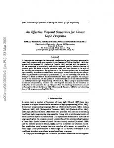
In this section we describe in detail the implementation of the framework. Our tool has a main front-end accepting in input a list of COLP programs and computing the joint fixpoints of such programs. This result is accomplished through several stages as depicted in Figure 1. In particular the overall process can be segmented into three big steps: 1. Converting a given set of COLP programs into classic propositional logic programs. 2. Generating a single logic program whose stable models are in one-to-one correspondence with the joint fixpoints of the input COLP programs.
8
Fig. 1. JFP → SM mapping stages and software modules implemented
3. Exploiting the DLV system in order to compute the stable models of such a program and then computing the (minimal) joint fixpoints. The first step is accomplished by the following two modules: 3.1
The Module colp2lp
Input: a list of non propositional COLP programs. Output: a list of non propositional classic logic programs. This module translates a non propositional COLP program into a classic logic program, exploiting the conversion rules described in [1]. In particular all okay and okay group predicates are recognized and accordingly expanded into classic rules. Moreover each integrity constraint is mapped to a rule whose head atom doesn’t occur in any other program. With regard to the beginning example, the COLP PDad is translated into the following classic logic program: twin airbag ← abs system ← city ← high disp ← air cond ← metal ← cd ←
city high disp, diesel air cond, high disp metal cd
As a further example, the statement okay group(metal,cd) included in the program PCharlie is converted into the following couple of rules: metal ← metal, cd cd ← metal, cd
9
3.2
The Module ground
Input: a list of non propositional classic logic programs. Output: a list of propositional classic logic programs. The mapping proposed in [1] works only with propositional programs. As a consequence, in order to give practical relevance to the implementation, we have to deal with the non trivial issue of grounding. Observe that if we have in input a set of non propositional COLP programs then the straight application of the mapping presented in Section 2.4 may produce unsafe rules. A program rule is safe if each variable occurring in that rule appears in at least one positive literal in the body of the same rule [7, 8]: in particular the rules included in the sets S1 , S3 and C are possibly unsafe because variables may occur as negative literals inside the body of generated rules. Thus, for each input non propositional program it is necessary to produce the corresponding propositional version. By exploiting the tool Lparse [9–13] this module performs the required grounding on a given set of non propositional programs. However, a further issue has to be considered: Lparse is optimized to discard those rules whose instantiations have unsatisfiable bodies, i.e. when some literal in the body is not deducible. This kind of optimization is not applicable in case of the JFP semantics, where okay and okay group predicates generate rules discarded by Lparse but meaningful w.r.t. the JFP semantics. Let us show the above issue by the example of chat forum presented in [1]. In this example we have a chat forum involving a fixed set of users: Ann, Bob, Connie and Dan. Each user can specify complex requirements concerning the presence of other users in the forum. The following COLP program represents the requirements of the user Ann: in forum(ann) ← okay(in forum(dan)) ← okay group(in forum(bob),in forum(connie)) ← subject(soccer)
This program models the following specifications: Ann wants to enter in the forum and she tolerates the presence of Dan, but she does not require him. Moreover, the joint presence of Bob and Connie is tolerated, but only if soccer is a subject of the forum. The above okay and okay group predicates are translated as follows: in forum(dan) ← in forum(dan) in forum(bob) ← in forum(bob), in forum(connie), subject(soccer) in forum(connie) ← in forum(bob), in forum(connie), subject(soccer)
Finally, the knowledge about each user is enriched by a common knowledge base, defining the relationships user, day and subject. Furthermore the constraint that a chat forum must contain at least two users is also included:
10 user(ann) user(bob) user(connie) user(dan) subject(soccer) day(monday) ⊥ multiple chat
← ← ← ← ← ← ← not multiple chat ← in forum(X), in forum(Y), user(X), user(Y), X 6= Y
A straight use of Lparse in order to perform the grounding does not return a complete instantiation for the above non propositional rule because not all the in forum predicates are deducible from the program. This problem has been solved by enriching each non propositional program with a set of facts, each fact representing a literal occurring in the whole collection of logic programs. This way, Lparse is forced to generate a full instantiation for each non propositional rule. Finally we discard from each grounded program those facts which were previously absent in the non propositional version. Thus we obtain a propositional logic program with a complete instantiation (here we only show the relevant part): multiple multiple multiple multiple multiple multiple multiple multiple multiple multiple multiple multiple
3.3
chat chat chat chat chat chat chat chat chat chat chat chat
← ← ← ← ← ← ← ← ← ← ← ←
in in in in in in in in in in in in
forum(ann), in forum(ann), in forum(ann), in forum(bob), in forum(bob), in forum(bob), in forum(connie), forum(connie), forum(connie), forum(dan), in forum(dan), in forum(dan), in
forum(bob), user(ann), user(bob) forum(connie), user(ann), user(connie) forum(dan), user(ann), user(dan) forum(ann), user(bob), user(ann) forum(connie), user(bob), user(connie) forum(dan), user(bob), user(dan) in forum(ann), user(connie), user(ann) in forum(bob), user(connie), user(bob) in forum(dan), user(connie), user(dan) forum(ann), user(dan), user(ann) forum(bob), user(dan), user(bob) forum(connie), user(dan), user(connie)
The Module build J
Input: a collection of propositional logic programs. Output: a single logic program J(P1 , · · · , Pn ) whose stable models are in one-toone correspondence with the joint fixpoints of the input COLP programs. This modules implements the translation rules described in Section 2.4. Briefly, for each program Pi ∈ {P1 , · · · , Pn } the sets of rules S1 , S2 and S3 are generated. Afterwards the set C(P1 , · · · , Pn ) is created. Finally: Ã ! [ [ J(P1 , · · · , Pn ) = S1 (Pi ) ∪ S2 (Pi ) ∪ S3 (Pi ) C(P1 , · · · , Pn ) Pi ∈{P1 ,···,Pn }
is produced as a final result. In the following paragraphs the translation algorithm is shown and commented.
11
The Translation Algorithm
Algorithm Translate Input V ar: Set of atoms, P = {P1 , · · · , Pi , · · · , Pn }: Set of logic programs over V ar; Output J(P1 , · · · , Pn ): a program associated to the set P such that the stable models of J(P1 , · · · , Pn ) correspond to the joint fixpoints of P1 , · · · , Pn ; var S1 , S2 , S3 , C, Γ (P1 ), · · · , Γ (Pi ), · · · , Γ (Pn ): Set of rules, LSet, L: List of atoms; begin 1. for each integer i | ∃ a program Pi ∈ P do (* S1 and S3 are created *) 2. S1 = ∅; S2 = ∅; S3 = ∅; 3. for each atom a ∈ V ar do 4. let a1 be a new literal; a1 .setN ame(a.getN ame + “p” + int2string(i)); 5. let a2 be a new literal; a2 .setN ame(a.getN ame + “ 0 ” + “p” + int2string(i)); 6. let r be a new rule; r.setHead([a1 .getN ame]); r.setBody([not a2 .getN ame]); 7. let s be a new rule; s.setHead([a2 .getN ame]); s.setBody([not a1 .getN ame]); 8. S1 = S1 ∪ {r} ∪ {s}; 9. let a3 be a new literal; a3 .setN ame(“s” + a.getN ame + “p” + int2string(i)); 10. let a4 be a new literal; a4 .setN ame(“f ail” + “p” + int2string(i)); 11. let t be a new rule; t.setHead([a4 .getN ame]); 12. t.setBody([not a4 .getN ame, a3 .getN ame, not a1 .getN ame]); 13. let u be a new rule; u.setHead([a4 .getN ame]); 14. u.setBody([not a4 .getN ame, a1 .getN ame, not a3 .getN ame]); 15. S3 = S3 ∪ {t} ∪ {u}; 16. end for (* S2 is created*) 17. for each rule r ∈ Pi | r : a ← b1 , · · · , bn do 18. let l be a new literal; l.setN ame(“s” + a.getN ame + “p” + int2string(i)); 19. LSet = ∅; 20. for each bj ∈ Body(r) 21. let lj be a new literal; lj .setN ame(bj .getN ame + “p” + int2string(i)); 22. let LSet = LSet ∪ {lj }; 23. end for 24. let L = SetT oList(LSet); 25. let s be a new rule; s.setHead([l.getN ame]); s.setBody(L); 26. S2 = S2 ∪ {s}; 27. end for (* Γ (Pi ) is created*) 28. Γ (Pi ) = S1 ∪ S2 ∪ S3 ; 29. end for (* C(P1 , · · · , Pn ) is created *) 30. C = ∅; 31. let f be a new literal; f.setN ame(“f ail”); 32. for each atom a ∈ V ar do 33. for each integer i ∈ [1, n] do 34. let aPi be a new literal; aPi .setN ame(a.getN ame + “p” + int2string(i)); 35. for each integer j ∈ [1, n] do 36. if i 6= j then 37. let aPj be a new literal; aPj .setN ame(a.getN ame + “p” + int2string(j)); 38. let r be a new rule; r.setHead([f.getN ame]); 39. r.setBody([not f.getN ame, aPi .getN ame, not aPj .getN ame]); 40. C = C ∪ {r}; 41. end if 42. end for 43. end for 44. end for (* J(P1 , · · · , Pn ) is created *) 45. J = ∅; 46. for each integer i ∈ [1, n] do 47. J = J ∪ Γ (Pi ); 48. end for 49. J = J ∪ C; end.
12
Comments to the Algorithm W.l.o.g. we assume the logic programs P1 , · · · , Pn being defined over the same set V ar. Furthermore we assume V ar being part of the input. A more general scenario has been implemented where each logic program can be defined on a different set of atoms V ar(Pi ) not being part of the input, but built at run-time. Moreover the set V ar is generated as the union of all the sets V ar(Pi ). lines 2 - 8: For each program Pi these statements build the set S1 : lines 2 - 5: For each atom a ∈ V ar two literals aPi and a0Pi are created. Atoms and literals are treated as objects having an attribute name. We assume that two methods getN ame and setN ame exist which are used to read / write such attribute. The function int2string returns the string representation of an integer number. lines 6 - 8: For each atom a ∈ V ar two rules aPi ← not a0Pi and a0Pi ← not aPi are created. Rules are treated as objects having two attributes: a Head and a Body. The method setHead (resp. setBody) receives a list L = [l1 , · · · , ln ] of literals and sets the head (resp. the body) of a specified rule using the literals inside L. After being created the rules are added to the set S1 . lines 9 - 16: For each program Pi these statements build the set S3 : lines 9 - 10: For each atom a ∈ V ar two literals saPi and f ailPi are created. lines 11 - 16: For each atom a ∈ V ar two rules f ailPi ← not f ailPi , saPi , not aPi and f ailPi ← not f ailPi , aPi , not saPi are created. Finally those rules are added to the set S3 . lines 17 - 27: For each program Pi , the set S2 is created. In particular: lines 18 - 23: Each rule r of the form: a ← b1 , · · · , bn is renamed to a new rule s : saPi ← b1Pi , · · · , bnPi . A set LSet is used to temporarily store the literals from the body of s. lines 24 - 27: The set LSet is converted to a list L which is input to the method setBody. Then the rule s is added to the set S2 . line 28: For each program Pi a new program Γ (Pi ) = S1 ∪ S2 ∪ S3 is created. lines 30 - 44: The set C = C(P1 , · · · , Pn ) is created. In particular for each atom a ∈ V ar and for each couple of different programs Pi and Pj two new literals aPi , aPj and a rule of the form f ail ← not f ail, aPi , not aPj are created. Then those rules are added to C. lines 45 - 49: J(P1 , · · · , Pn ) is created as J = Γ (P1 ) ∪ · · · ∪ Γ (Pn ) ∪ C. At this stage we exploit the DLV system [7, 8] in order to compute the stable models of J(P1 , · · · , Pn ). 3.4
The Module parse SM
Input: the stable models of the program J(P1 , · · · , Pn ). Output: the joint fixpoints of P1 , · · · , Pn .
13
This module post-processes the output results from DLV. In particular it filters the stable models of J(P1 , · · · , Pn ) extracting the relevant atoms, i.e. those being part of JFP(P1 , · · · , Pn ). Finally the original names those atoms had within the COLP programs are restored, i.e. name prefixes and suffixes added by the translation process are discarded. For example, a stable model of J(P1 , · · · , Pn ) is the following: {s abs system P1, s twin airbag P1, s twin airbag P2, abs system P1, air cond 1 P1, cd P1, city P1, diesel 1 P1, high disp 1 P1, metal P1, petrol P1, twin airbag P1, s cd P1, s city P1, s metal P1, s petrol P1, abs system P2, air cond 1 P2, auto shift 1 P2, cd P2, city P2, diesel 1 P2, high disp 1 P2, metal P2, petrol P2, steering 1 P2, twin airbag P2, s abs system P2, s cd P2, s city P2, s metal P2, s petrol P2, abs system P3, air cond 1 P3, auto shift 1 P3, cd P3, city P3, diesel 1 P3, high disp 1 P3, metal P3, petrol P3, steering 1 P3, twin airbag P3, s abs system P3, s cd P3, s city P3, s metal P3, s petrol P3, s twin airbag P3}
where all atoms having a prefix s (the supported atoms) jointly occur with those without the prefix (the fixpoints) as an effect of the rules in S3 . Moreover the suffix Pi indicates which logic program an atom comes from. From this stable model the following joint fixpoint is extracted: {abs system, twin airbag, cd, city, metal, petrol}
3.5
The Module find MJFP
Input: the joint fixpoints of P1 , · · · , Pn . Output: the minimal joint fixpoints of P1 , · · · , Pn . The set of minimal joint fixpoints MJFP(P1 , · · · , Pn ) is built in a bottom-up fashion. At the beginning MJFP is empty and the input joint fixpoints are sorted by ascending cardinality, i.e. the number of included atoms. Fixpoints having the minimum cardinality are also minimal, thus they are directly included in MJFP. The remaining fixpoints are separately processed: a fixpoint is discarded if an element of MJFP exists which is included in it, otherwise it is added to MJFP. In the following paragraphs the algorithm is shown and commented. 3.6
MJFP Search Algorithm
Algorithm MJFP Search Input JF P (P1 , · · · , Pn ): Set of joint fixpoints of the programs P1 , · · · , Pn . Output M JF P (P1 , · · · , Pn ): Set of minimal joint fixpoints of the programs P1 , · · · , Pn . var L: List of fixpoints; mincard: Integer; discard: Boolean; begin 1. for each element f ∈ JF P (P1 , · · · , Pn ) do 2. L.append(f ); 3. end for 4. sort(L, cardinality, ascending); 5. mincard = card(L.f irst); M JF P = ∅; 6. for each element l in list L do 7. if card(l) = mincard then M JF P = M JF P ∪ {l}; 8. else begin
14 9. 10. 11. 12. 13. 14. 15. end.
discard = f alse; for each element m ∈ M JF P do if {m} ⊆ {l} then discard = true; end for if not discard then M JF P = M JF P ∪ {l}; end; end for
Comments to the Algorithm lines 1 - 3: The elements of JF P (P1 , · · · , Pn ) are copied in a list L. line 4: The elements of L are sorted by ascending cardinalities, i.e. number of included atoms. lines 6 - 15: This is the core of the algorithm, in particular: line 7: Fixpoints having the minimum cardinality are added to MJFP. lines 8 - 12: Fixpoints not having the minimum cardinality are checked for set inclusion minimality: if any of them includes an element of MJFP then it is discarded. lines 13 - 15: Fixpoints which are not discarded are minimal, so they are added to MJFP. Furthermore, even though the algorithm works in polynomial time, space complexity represents a concrete drawback. In fact all joint fixpoints have to be computed before finding the minimal ones, i.e. exponential space is required. As discussed in the next section, an interesting issue to be investigated is of course the problem of encoding minimality directly into the original programs in order to avoid space exploitation generated by the previous approach. However, this approach may have significance every time the number of JFPs is small, that is a plausible case, since it corresponds to have heterogeneous agents’ requirements.
4
Conclusions and Future Work
In this paper we described a framework which implements the joint fixpoint semantics introduced in [1] on the top of the DLV system. This semantics is suitable to model joint decisions of agents represented by logic programs. In order to meet this target we realized software tools which receive in input a collection of COLP programs, each representing the requirements and desires of an agent, and generate a single program whose stable models are in one-to-one correspondence to the COLPs’ joint fixpoints. Those stable models are computed exploiting the DLV system. As a final result we compute the joint fixpoints of the input COLP programs, i.e. the fixpoints which are common to all the input COLP programs. Those joint fixpoints represent a common agreement among the agents. Moreover we embedded an option to compute the minimal joint fixpoints, i.e. the joint fixpoints containing the minimum number of atoms required to meet a common agreement between the agents. It is easy to see that the computational complexity of the implementation reaches the theoretic one. It has
15
been pointed out that searching for the minimal joint fixpoints requires an exponential space, thus a new scheme for the mapping from joint fixpoint semantics to stable model semantics has to be investigated in order to directly produce the minimal joint fixpoints. Grounding is another issue that could be solved in an alternative way: again, by changing the translation scheme it could be possible to avoid the generation of unsafe rules within the sets S1 , S3 and C. This way the translation process could directly work with non propositional COLP programs, thus avoiding the overhead produced by the ground instantiations. This is left for future investigations.
References 1. Buccafurri, F., Gottlob, G.: Multiagent Compromises, Joint Fixpoints and Stable Models. Computational Logic: From Logic Programming into the Future (In honour of Bob Kowalsky), Ed. A. Kakas and F. Sadri, Springer Verlag (2002) 2. Baral C., Gelfond M.: Logic Programming and Knowledge Representation. Journal of Logic Programming 19-20, (1994) 73–148 3. Minker J., Seipel D.: Disjunctive Logic Programming: A Survey and Assessment. Computational Logic: From Logic Programming into the Future (In honour of Bob Kowalsky), Ed. A. Kakas and F. Sadri, Springer Verlag (2002) 4. Kolaitis, P.G., Papadimitriou, C.H.: Why not Negation by Fixpoint? Journal of Computer and System Sciences 43(1), (1991) 125–144 5. Gelfond, M., Lifschitz, V.: The Stable Model Semantics for Logic Programming. Proceedings of the 5th International Conference on Logic Programming, MIT Press, Cambridge, (1988) 1070–1080 6. Baral C.: Knowledge Representation, Reasoning and Declarative Problem Solving. Cambridge University Press, (2003) 7. Leone, N., Pfeifer, G., Faber, W., Calimeri, F., Dell’Armi, T., Eiter, T, Gottlob, G., Ianni, G., Ielpa, G., Koch, C., Perri, S., and Polleres, A.: The DLV System. Proceedings of the 8th European Conference on Logics in Artificial Intelligence (JELIA) n.2424 in Lecture Notes in Computer Science, (2002) 537–540 8. Bihlmeyer, R., Faber, W., Ielpa, G., and Pfeifer, G.: DLV - User Manual. Available at: http://www.dlvsystem.com 9. Syrj¨ anen, T.: Lparse 1.0 User’s Manual. Available at: http://www.tcs.hut.fi/Software/smodels/lparse.ps.gz 10. Niemel¨ a, I., Simons, P.: Smodels - an Implementation of the Stable Model and Wellfounded Semantics for Normal Logic Programs. Proceedings of the 4th International Conference on Logic Programming and Non-Monotonic Reasoning (LPNMR ’97), Lecture Notes in Computer Science, Vol. 1265. Springer-Verlag, Dagstuhl, Germany (1997) 420–429 11. Niemel¨ a, I., Simons, P., and Syrj¨ anen, T.: Smodels: a system for answer set programming. Proceedings of the 8th International Workshop on Non-Monotonic Reasoning, Breckenridge, Colorado, USA, (2000) anen, T.: Implementation of Local Grounding for Logic Programs with Sta12. Syrj¨ ble Model Semantics. Technical Report, Helsinki University of Technology, Digital Systems Laboratory, (1998) a, I.,and Soinen, T.: Extending and Implementing the stable 13. Simons, P.,Niemel¨ model semantics. Artificial Intelligence 138, (2002)