Implicitization of Parametric Curves by Matrix Annihilation

Implicitization of Parametric Curves by Matrix Annihilation Hulya Yalcin✝, Mustafa Unel✝✝, William Wolovich✝ ✝

✝✝

Division of Engineering, Brown University, RI Center for Computational Vision and Control, Yale University, CT

Abstract Both parametric and implicit representations can be used to model 2D curves and 3D surfaces. Each has certain advantages compared to the other. Implicit polynomial (IP) methods are not as popular as parametric procedures because the lack of general procedures for obtaining IP models of higher degree has prevented their general use in many practical applications. In most cases today, parametric equations are used to model curves and surfaces. One such parametric representation, elliptic Fourier Descriptors (EFD) has been widely used to represent 2D and 3D curves, as well as 3D surfaces. Although EFDs can represent nearly all curves, it is often convenient to have an implicit algebraic description F(x,y)=0, especially for determining whether given points lie on the curve. Algebraic curves and surfaces also have proven very useful in many model-based applications. Various algebraic and geometric invariants obtained from these implicit models have been studied rather extensively. In this paper, we present a new non-symbolic implicitization technique called the matrix annihilation method, for converting parametric Fourier representations to implicit polynomial form.

1.

INTRODUCTION

In general, any closed curve can be described in terms of a set of two (or three for space curves) Fourier series whose coefficients are called elliptic Fourier descriptors (EFDs). The advantages of using EFDs are that the shape information is concentrated in the low frequency parts [1-5], hence shape can be described by the first few coefficients. Invariants derived from EFDs have been used for identification [5,6]. Algebraic curves/surfaces have also proven to be very useful for shape representation [7,8]. In the past few years, implicit representations have been used more frequently, allowing a better treatment of several problems. One example is the point classification problem, which is easily solved with the implicit representation since it consists of a simple evaluation of the implicit functions. Invariants associated with these models have also been employed in several modelbased vision and pattern recognition applications [9-13]. However, there is very little in the literature on higher degree IP models for large or entire free-form shapes because of the lack of tractable computational procedures for obtaining and analyzing such models. The implicit polynomial that defines a curve is not easily determined. Although several different fitting algorithms have been proposed thus far for directly determining IP models from point data sets, the computational cost of many of them is quite high because of the nonlinear optimization procedures required to obtain acceptable fits. Lack of stability of parameters has been another weakness. The problem of excessive number of parameters in implicit representations was first studied in [13]. The 3L fitting algorithm [14] exhibits significantly improved curve representation accuracy and stability. However, there is significant value to further improvement in coefficient stability to make algebraic curves more generally and robustly applicable

0-7803-7622-6/02/$17.00 ©2002 IEEE

for object recognition. Instead of obtaining algebraic curve representations directly from points, it is also possible to convert parametric equations (which may be obtained from boundary points) to implicit ones. Sederberg has extensively studied the problem of converting parametrically defined curves to implicit form using elimination theory, which involves computing the determinant of Sylvester’s matrix [15-17]. Later, Hong employed Sylvester’s matrix –also known as the resultant method- for a particular class of problems involving trigonometric polynomials, taking advantage of their special structure [18]. A significant disadvantage of implicitization by Sylvester’s matrix elimination method is that it involves computing the determinant of a matrix which contains symbolic variables. Ercil et al [19] studied the problem of converting between parametric and implicit forms based on polar/spherical coordinate representations. However, their technique is valid only for star-shaped objects. In this paper, we present a new, non-symbolic implicitization technique, called the matrix annihilation method, for converting parametric Fourier representations to algebraic (implicit polynomial) representations. We should note that our method is numerical, so that we can obtain higher order polynomial curves than previously possible through implicitization. Furthermore, our procedure is computationally efficient. The structure of the paper is as follows: Section 2 reviews implicitization by Sylvester’s matrix. In section 3, our approach for implicitization is described. Section 4 illustrates our procedure using several examples. Section 5 describes two vision-based examples, and some concluding remarks are given in Section 6. 2.

Review of Implicitization by Sylvester’s Matrix

Sylvester’s matrix elimination method [17] can be used to implicitize parametric polynomial curves such as x=a2t2+a1t+a0 and y=b2t2+b1t+b0. In particular, if we re-write these equations as a2t2+a1t+(a0-x)=0 and b2t2+b1t+(b0-y)=0, the resultant of these two polynomials is then defined by the determinant of Sylvester’s matrix, namely a 2  0 S= b 2   0

a1 a2 b1 b2

S = b 22 x 2 − 2a 2 b 2 xy + a 22 y 2  + (2a 2 b 2 b 0 + a 1 b1 b 2 - a 2 b12 - 2a 0 b 22 )x  a1 a 0 − x ⇒ + (a 2 b1a 1 + 2a 2 b 2 a 0 - 2a 22 b 0 − a 12 b 2 )y b0 − y 0  + (a 1 b 2 − a 2 b1 )(a 1 b 0 − a 0 b1 )  b1 b 0 − y  2 + (a 2 b 0 − a 0 b 2 ) = 0

a0 − x

0

an implicit algebraic curve that is equivalent to the parametric curve. In general, if x and y are polynomials of degree p, the corresponding algebraic curve also will have degree p. To further illustrate this procedure, consider the parametric curve defined by the equations: x = 0.4 + 0.5 cos t − 2 sin 2 t and

III - 889

IEEE ICIP 2002

y = 0.6 + 0.2 sin t − 2 sin 2 t . By substituting the following equivalent complex relations for coskt and sinkt sin kt = (e ikt − e − ikt )/ 2

cos kt = (e ikt + e − ikt )/ 2 ,

(2.1)

where A k = (a k − ib k )/ 2 , B k = (a k + ib k )/ 2 , C k = (c k − id k )/ 2 ,

D k = (c k + id k )/ 2 for k=1,…,n, with A 0 = a 0 and C 0 = c 0 . These equations can be expressed in a more compact form by substituting z for eit,

it

and then substituting z=e and mutiplying both equations by z2 in order to make all z powers positive, we obtain

x (z ) = A o + ∑ (A k z k + B k z − k ) ≡ ∑ g[ k ]z k

0 = iz 4 + 0.25z 3 + (0.4 − x )z 2 + 0.25z − i

y(z ) = C o + ∑ (C k z k + D k z − k ) ≡ ∑ h[ k ]z k

0 = 0.35z 4 − 0.1iz 3 + (0.6 − y )z 2 + 0.1iz + 0.35

n

n

k =1

k =− n

n

n

k =1

k=−n

where A k  g[k ] = A 0 B  k

Using elimination theory, the determinant of Sylvester’s matrix is then defined by i 0 0 0   −i 0.25 0.4 − x 0.25   −i 0.25 0.4 − x 0.25 i 0 0   0  0 −i 0 0.25 0.4 − x 0.25 i 0 ,   − − 0 0 0 i 0 . 25 0 . 4 x 0 . 25 i  S =  0.35 0.1i 0.6 − y − 0.1i 0.35 0 0 0    0.35 0.1i 0.6 − y − 0.1i 0.35 0 0   0  0 0 0.35 0.1i 0.6 − y − 0.1i 0.35 0    0 0 0 0.35 0.1i 0.6 − y − 0.1i 0.35

if k > 0 if k = 0 if k < 0

xy = x (z )y(z ) = Ζ{g[k ] ∗ h[k ]},

−160.35y3 −1.332x2 +15.726xy + 79.04y2 + 1.578x + 24.698y − 3.736 = 0

1.6 Parametric curve Our implicit curve

 1     x   y   2   x   xy   2 =  y   x3        d −1  xy   yd    Γ

1.2

1.2 1

1 0.8

0.8 y

y

0.6

0.6

0.4

0.4

0.2

0.2 0

0

-0.2

-0.2

-0.4

-0.4

-2

-1

0

1

2

3

-2

-1.5

-1

-0.5

x

0

0.5 x

1

1.5

2

2.5

3

Figure 1 (a) Parametric curve and implicit curve obtained by Sylvester’s elimination method, (b) parametric curve and implicit curve obtained by matrix annihilation method are superimposed.

3.

Our Approach: Implicitization by Matrix Annihilation

  L      P = Pˆ         

x ( t ) = a o + ∑ (a k cos kt + b k sin kt ) n

k =1 n

(3.1)

k =1

where (ao,co) is the center of the curve. Using (2.1), we can express (3.1) as n

x ( t ) = A 0 + ∑ A k e ikt + B k e − ikt k =1 n

y( t ) = C 0 + ∑ C k e ikt + D k e − ikt

(3.2)

k =1

1

The coefficients of coskt and sinkt in (3.1) can be uniquely determined from an ordered sequence of points which describe the boundary of a curve using the relations given in Chapter 2 of [6]. We will assume here that this operation has been performed and, therefore, that the Fourier coefficients are known.

0 0 1 0 0   g   − nd  z   h      g∗g       z −1   g∗h     h∗h   1     z1   g ∗g∗g             z nd   g h h ∗ ∗ ∗       * d −1   z h h h  ∗ ∗ ∗    d    P : Convolution Matrix

(3.4)

or simply Γ = Pz for some complex (d + 1)(d + 2) / 2 × (2dn + 1) matrix P. We next re-write P as

Consider an n-harmonic elliptic Fourier descriptor representation of any 2-D curve, namely1

y( t ) = co + ∑ (c k cos kt + d k sin kt )

y 2 = y(z )y(z ) = Ζ{h[ k ] ∗ h[ k ]}.

The monomials x p y q for different p and q values can be found similarly. We can therefore write

that is shown in Figure 1(a). 1.4

if k > 0 if k = 0 if k < 0

convolution property of the z-transform: “if g[k] ⇔ x(z) and h[k] ⇔ y(z) then g[k]∗h[k] ⇔ x(z)y(z)”. Note that convolution in discrete-time domain corresponds to multiplication in the zdomain. For example, x 2 = x (z )x (z ) = Z{g[ k ] ∗ g[ k ]},

f4 (x, y) = x4 +16.327x2 y2 + 66.639y4 −1.6x3 −19.657x2 y −13.061xy2

Parametric curve Sylvesters implicit curve

C k  h[k ] =  C 0 D  k

If the g and h sequences are written as vectors g = [B n  B1 A 0 A 1  A n ] and h = [D n  D1 C 0 C1  C n ] , & & (3.3) can then be re-written as x (z ) = g ⋅ z and y(z ) = h ⋅ z where * z T = [z − n  z −1 1 z  z n ]. We next employ the time

which implies the (monic) quartic implicit polynomial curve

1.4

(3.3)









  L

  

  

  

                                         L              L 

for some unique, real (d + 1)(d + 2) / 2 × (2d 2 + 1) matrix Pˆ . We then determine the “largest” (d+1)(d+2)/2-1=d(d+3)/2 columns of Pˆ via an orthogonal-triangular decomposition

III - 890

defined by QR = PˆE , where Q is a unitary matrix, R is an upper triangular matrix whose diagonal elements are of decreasing absolute value, and E is a permutation matrix which orders the columns of PˆE in correspondence with those of QR . The unique unit vector ν that annihilates the first d (d + 3) / 2 columns ~ of PˆE , which we will define as P , then yields an appropriate (non-monic) implicit polynomial function as the product ν Γ = f d ( x , y) = 0 . The Matlab routines “qr” and “null” are used to perform the required computations. Implicitization of truncated Fourier descriptors with n harmonics implies an algebraic equation of degree d=2n. 4.

f4 (x, y) = x4 + 16.327x2 y2 + 66.639y4 − 1.6x3 − 19.657x2 y − 13.061xy2 − 160.35y3 − 1.332x2 + 15.726xy + 79.04y2 + 1.578x + 24.698y − 3.736 = 0

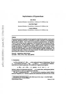
~ that is shown in Figure 1(b). The annihilated matrix P defined by our method is 15x14, and it takes 0.06 seconds to implicitize. Sylvester’s matrix is 8x8, but it takes 7.25 seconds to implicitize. 4.2. Convert 3 harmonic EFD curve to 6th degree IP curve: The parametric curve in Figure 2(a) is represented by the following Fourier coefficients: a 0 = -0.0906 , c 0 = -0.1194

[a [b [c [d

SOME EXAMPLES

In this section, we present the implicitization of several curves, some with strong discontinuities and some self-intersecting. Given an ordered sequence of points on each curve, we first computed the parametric Fourier coefficients of the curve. We then implicitized the curves both by our matrix annihilation method and Sylvester’s elimination method. Both implicitization methods were implemented in Matlab. For Sylvester’s elimination method, we used the Symbolic Toolbox of Matlab and/or Maple. Assuming that n harmonic Fourier coefficients are used to represent the curve, our method involves computing the ~ annihilating vector of P , whereas implicitization by Sylvester’s elimination method involves computing the determinant of a 4nx4n symbolic matrix. As the number of harmonics used to represent curves increase, the computation time increases for both methods. However, since Sylvester’s elimination method involves symbolic computation, the computation time increases faster than our method, as we will show.

1

a2

1

b2

a 3 ] = [-0.1827 -0.1902 -0.1302] b 3 ] = [-0.3267 -0.1753 -0.1568]

1

c2

1

d2

c 3 ] = [-0.3383 -0.153 -0.0971]

d 3 ] = [0.3385 0.0992 -0.1589]

The 6th degree IP obtained by both our annihilation method and Sylvester’s elimination method is the same, namely f (x, y ) = x 6 - 6.4992x 5 y + 17.6741x 4 y 2 - 25.7403x 3 y 3 + 21.1742x 2 y 4 - 9.3283xy 5 + 1.7195y 6 - 2.5056x 5 + 10.5328x 4 y - 16.0141x 3 y 2 + 10.0422x 2 y 3 - 1.6236xy 4 - 0.4356y 5 + 0.1532x 4 + 3.6857x 3 y - 7.8187x 2 y 2 + 4.8756xy 3 - 0.7753y 4 + 2.1925x 3 - 2.9669x 2 y + 0.8362xy 2 + 0.0254y 3 + 0.6077x 2 - 0.5863xy + 0.0803y 2 - 0.0041x + 0.0599y - 0.0096 = 0

~ and shown in Figure 2(a). The annihilated matrix P defined by our method is 28x27 and it takes 0.06 seconds to implicitize. Sylvester’s matrix is 12x12, but it takes 8.46 seconds to implicitize.

4.1. Convert 2 harmonic EFD curve to 4th degree IP curve: To illustrate our matrix annihilation procedure, consider the earlier parametric curve defined by

Parametric curve Our implicit curve Sylvesters implicit curve

0.6

1 0.8

Parametric curve Our implicit curve

0.4

0.6 0.2

0.4 0.2

y = 0.6 + 0.2 sin t + 0.7 cos 2 t

y

y

x = 0.4 + 0.5 cos t − 2 sin 2 t ,

0

-0.2

whose Fourier coefficients are given by a 0 = 0.4 , c 0 = 0.6

[a [c

1

1

a 2 ] = [0.5 0]

c 2 ] = [0 0.7]

[b [d

1

1

0 -0.2 -0.4

-0.4

-0.6 -0.6

-0.8

b 2 ] = [0 −2]

-0.8 -1

-0.5

0 x

d 2 ] = [0.2 0]

The complex Fourier coefficients are then determined to be A 0 = 0.4 , C = 0.6 , [A 1 A 2 ]= [0.25 i], [B1 B 2 ]= [0.25 − i ], [C1 C 2 ]= [−0.1i 0.35], [D1 D 2 ]= [0.1i 0.35] . The g and h sequences are then defined as

0.5

-1 -1

-0.8

-0.6

-0.4

-0.2

0

0.2

0.4

0.6

0.8

x

Figure 2 (a) Parametric curve, implicit curve (circles) obtained by matrix annihilation and implicit curve (dots) obtained by Sylvester’s elimination methods are superimposed. (b) Parametric curve and implicit curve (circles) obtained by matrix annihilation method are superimposed.

0

g = [−i 0.25 0.4 0.25 i] ,

h = [0.35 0.1i 0.6 −0.1i 0.35]

~ which subsequently imply (3.4). The (15x14) P matrix is then determined as outlined above and the vector that annihilates this matrix is found to be ν = [− 0.0191 0.0081 0.1265 − 0.0068 0.0806 0.4049 − 0.0082 − 0.1007 − 0.0669 − 0.8215 0.0051 0 0.0836 0 0.3414]

Reordering the terms in lexicographic order and dividing by the leading coefficient, we obtain the following monic implicit polynomial curve

4.3. Convert 6 harmonic EFD curve to 12th degree IP curve: The parametric curve in Figure 2(b) is represented by following Fourier coefficients: a 0 = −0.057 , c 0 = −0.0157

[a , a , a , a , a , a ]= [− .5224,−.0574,0.083,0.1513,0.0262,0.1703] [b , b , b , b , b , b ]= [− .09,0.089,0.0258,−.0154,0.0251,−.0113] [c , c , c , c , c , c ]= [− .1396,0.0652,0.0682,0.0843,−.0832,0.0176] [d , d , d , d , d , d ] = [0.6211,0.0893,0.0938,0.1858,−.0864,−.1864] 1

2

1

3

2

1

3

2

1

4

5

4

3

5

4

2

3

6

6

5

4

6

5

6

th

The 12 degree implicit polynomial2 obtained by our annihilation method is shown in Figure 2(b). The annihilated 2

The coefficients of the implicit polynomial equations which define our remaining curves can be obtained from the authors.

III - 891

~ matrix P defined by our method is 91x90 and it takes 1.21 seconds to implicitize. When the number of harmonics used to represent a curve is greater than 4 (degree of target implicit polynomial greater than 8), we found that implicitization by Sylvester’s elimination method is impossible using Matlab. 5.

Extracting Shape Features from IP Models

Once an implicit polynomial that defines the shape of an object has been determined, it can be used for object recognition in a variety of ways. As shown in [12-14], algebraic invariants can be defined and determined directly from implicit polynomial models. These invariants can then be used to compare and identify similar objects. Implicit polynomial representations can also be used to characterize the local geometry of a curve, i.e curvature. The classical approach in curvature computation is to use local curve fitting or structural models for a local neighborhood of the curve, which typically perform poorly in the vicinity of singularities. To avoid this problem, we use the implicit representation obtained by our matrix annihilation method to compute curvature of a curve and determine whether the objects are the same or similar. -1 -0.8 -1.5

-0.6 -0.4

-1

-0.2 -0.5

0 0.2

0

0.4 0.5

0.6 0.8

1

1 -1.5

-1

-0.5

0

0.5

1

1.5

1.5 -1.5

-1

-0.5

0

0.5

1

1.5

Figure 3 (a) Carpal3d_01_01 image. (b) Contour points of the first bone (circle) and 10th degree IP curve obtained by our matrix annihilation (solid). (c) Contour points of the second bone (circle) and 8th degree IP curve (solid).

Figure 4 (a) Cell image, (b) contour points of the cell (circle) and 10th degree IP (5 harmonic) (solid).

Consider the carpal bone image depicted in Figure 3 (a). Using our matrix annihilation algorithm, a 10th degree IP curve is determined that describes the boundary of the first bone and an 8th degree IP curve is determined that describes the boundary of the second bone, which is depicted in Figure 3 (b) and (c) respectively. Similarly, implicit representation of the cell in Figure 4(a) is shown in Figure 4 (b). Computing the curvature of carpal bone shapes from their implicit representation together with perpendicular distance computation, we aim to use such information to quantify the degree to which the shape of a particular carpal bone differs from that of an ideal one. 6.

CONCLUSIONS

Implicit polynomial representations are very useful for modeling given point data sets, and numerous papers have been written which illustrate their importance in image understanding and

object recognition. A variety of methods have been devised for directly fitting given data sets to implicit polynomial curves and, although such methods are continually being refined and improved, alternative implicitization procedures are equally important and useful. In this report, we have demonstrated a new matrix annihilation method for efficiently converting curves defined by elliptic Fourier descriptors to algebraic ones. As we have explicitly illustrated, our matrix annihilation method works very well and efficiently in many higher order cases where symbolic-based methods fail. We are currently working on extending our matrix annihilation method to implicitize both 2D curves and 3D surfaces that are defined by a variety of parametric representations. We also are investigating the use of these implicit models in a variety of computer vision applications. The two simple examples in Section 5 were given to illustrate the potential utility of our method, and spatial limitations prevent us from presenting additional computer vision applications here. 7.

REFERENCES

[1] T.P. Wallace and O.R. Mitchell, “Analysis of Three-Dimensional Movement Using Fourier Descriptors” IEEE Trans. Pattern Analysis and Machine Intelligence, vol.2, no.6, pp. 583-588, 1980. [2] F.P. Kuhl and C.R. Giardina, “Elliptic Fourier Features of a Closed Contour,” Computer Graphics and Image Processing, vol.18, 1982. [3] C.T. Zahn and R.Z. Roskies, “Fourier Descriptors for Plane Closed Curve,” IEEE Trans. Computers, vol. 21, no. 3, pp. 269-281,1972. [4] G.H. Granlund, “Fourier Preprocessing for Hand Print Character Recognition,” IEEE Trans. Computers, vol. 21, pp. 195-201, 1972. [5] C.S. Lin and C.L. Hwang, “New Forms of Shape Invariants From Elliptic Fourier Descriptors,” Pattern Recognition, 20(5):535-545, 1987. [6] P.E. Lestrel, Fourier Descriptors and Their Applications in Biology, Cambrigde Univ. Press, 1997. [7]G.Taubin, F.Cukierman, S.Sullivan, J.Ponce and D.J. Kriegman, “Parameterized Families of Polynomials for Bounded Algebraic Curve and Surface Fitting,” IEEE Trans. Pattern Analysis and Machine Intelligence, 16(3):287-303, March 1994. [8] D. Keren, D. Cooper and J. Subrahmonia, “Describing Complicated Objects by Implicit Polynomials,” IEEE Trans. Pattern Analysis and Machine Intelligence, Vol. 16, pp. 38-53, 1994. [9] W. A. Wolovich, and Mustafa Unel, “The Determination of Implicit Polynomial Canonical Curves,” IEEE Transactions on Pattern Analysis and Machine Intelligence, Vol. 20 (8), 1998. [10] M. Unel, and W. A. Wolovich, “Pose Estimation and Object Identification Using Complex Algebraic Representations,” Pattern Analysis and Applications Journal, Vol. 1 (3), 1998. [11] M. Unel and W. A. Wolovich, “On the Construction of Complete Sets of Geometric Invariants for Algebraic Curves,” Advances in Applied Mathematics 24, 65-87, 2000. [12] M. Unel and W. A. Wolovich, “A New Representation for Quartic Curves and Complete Sets of Geometric Invariants,” Int. Jour. of Pattern Recognition and Artificial Intelligence, 13 (8), 1999. [13] J., Subrahmonia, D. B. Cooper, and D. Keren, “Practical Reliable Bayesian Recognition of 2D and 3D Objects using Implicit Polynomials and Algebraic Invariants,” IEEE Transactions on Pattern Analysis and Machine Intelligence, 18(5):505-519, 1996. [14] M.M. Blane, Z. Lei, H. Civi and D. B. Cooper, “The 3L Algorithm for Fitting Implicit Polynomial Curves and Surfaces to Data,” IEEE Transactions on Pattern Analysis and Machine Intelligence, 22(3), 2000. [16] T.W.Sederberg, “Implicit and Parametric Curves and Surfaces for Computer Aided Geometric Design,” Ph.D. Thesis, Dept. Mechanical Engineering, Purdue University, 1983. [17] T.W.Sederberg and D.C.Anderson, “Implicit Representation of Parametric curves and Surfaces,” Comput. Vision&Graph. Image Process., 28(1):72-84, 1984. [18] T. W. Sederberg and R.N. Goldman, “Algebraic geometry for Computer-aided Geometric Design,” IEEE Comput. Graph. Appl. 6(6), 52-59, 1986. [19] H. Hong, “Implicitization of Curves Parametrized by Generalized Trigonometric Polynomials,” Proceedings of Applied Algebra, Algebraic Algorithms and Error Correcting Codes (AAECC-11), pp. 285-296, 1995. [20] C. Unsalan and A. Ercil, “Conversions between Parametric and Implicit Forms Using Polar/Spherical Coordinate Representations,” Computer Vision and Image Understanding 81, 1-25 (2001).

III - 892