Improved Algorithms and Complexity Results for Power Domination in

Improved Algorithms and Complexity Results for Power Domination in Graphs∗ Jiong Guo†

Rolf Niedermeier†

Daniel Raible‡

July 3, 2007

Abstract The NP-complete Power Dominating Set problem is an “electric power networks variant” of the classical domination problem in graphs: Given an undirected graph G = (V, E), find a minimum-size set P ⊆ V such that all vertices in V are “observed” by the vertices in P . Herein, a vertex observes itself and all its neighbors, and if an observed vertex has all but one of its neighbors observed, then the remaining neighbor becomes observed as well. We show that Power Dominating Set can be solved by “bounded-treewidth dynamic programs.” For treewidth being upper-bounded by a constant, we achieve a linear-time algorithm. In particular, we present a simplified linear-time algorithm for Power Dominating Set in trees. Moreover, we simplify and extend several NPcompleteness results, particularly showing that Power Dominating Set remains NP-complete for planar graphs, for circle graphs, and for split graphs. Specifically, our improved reductions imply that Power Dominating Set parameterized by |P | is W[2]-hard and it cannot be better approximated than Dominating Set. Key Words. Design and analysis of algorithms, computational complexity, parameterized complexity, fixed-parameter algorithms, graph algorithms, graphs of bounded treewidth, (power) domination in graphs.

1

Introduction

Domination is a central theme in graph theory [23, 22, 24]. The basic problem is: given an undirected graph G = (V, E), determine a minimum-size vertex set ∗ A preliminary version of this paper appears in the proceedings of the 15th International Symposium on Fundamentals of Computation Theory (FCT’05), volume 3623 in LNCS, pages 172–184, Springer-Verlag, 2005. Work supported by the Deutsche Forschungsgemeinschaft (DFG), Emmy Noether research group PIAF (fixed-parameter algorithms), NI 369/4. Significant portions of this work were done while all authors were affiliated with the Universit¨ at T¨ ubingen. † Institut f¨ ur Informatik, Friedrich-Schiller-Universit¨ at Jena, Ernst-Abbe-Platz 2, D07743 Jena, Germany. {guo,niedermr}@minet.uni-jena.de ‡ Abteilung Informatik/Wirtschaftsinformatik, Fachbereich IV, Universit¨ at Trier, D-54286 Trier, Germany. [email protected]

1

D ⊆ V such that each vertex v is contained in D or v is a neighbor of at least one vertex in D. The corresponding decision problem Dominating Set (DS) is NPcomplete and W[2]-complete [16, 30]. Unless NP-hard problems have slightly superpolynomial-time algorithms, Dominating Set is not polynomial-time approximable better than Θ(log |V |) [17]. Numerous variations of Dominating Set exist. For instance, Connected Dominating Set—which recently has received particular interest for routing in ad-hoc networks [2]—additionally requires that the dominating set D induces a connected subgraph of G. Opposite to Dominating Set, Connected Dominating Set carries some form of non-locality: the correctness of the connected dominating set cannot be decided by locally checking every direct neighborhood. In this work, we study another “non-local” variant of domination which appears in electric power networks [12, 21]—Power Dominating Set (PDS). This variant is motivated by monitoring an electric power network, where one is asked to place a minimum number of so-called phase measurement units (PMU) at some locations in the system to measure the state variables (for example, the voltage magnitude). Since the monitoring PMU devices are expensive, to save costs one naturally comes to the minimization problem modelled by PDS. Intuitively, in comparison with Connected Dominating Set we have a more complex degree of non-locality in PDS. Whereas Connected Dominating Set only refers to a property of the solution set, PDS has the non-locality in its domination mechanism: A vertex may dominate vertices at arbitrary distance when certain conditions are fulfilled. For DS, we have one “observation rule” concerning vertices in the dominating set: these vertices observe (dominate) themselves and all their neighbors (and nothing else). The goal is to get all vertices observed by a minimum number of observers. By way of contrast, we have an additional observation rule in the case of PDS. This rule says that for an already observed vertex whose all but one neighbors are already observed, the one remaining neighbor becomes observed as well.1 Note that the second observation rule brings in non-locality. The graph-theoretical and algorithmic study of PDS was initiated by Haynes et al. [21] and has been further pursued for special cases [12, 15, 29]. Haynes et al. showed that PDS is NP-complete for general graphs as well as for bipartite and chordal graphs. Moreover, they presented a linear-time algorithm to solve PDS in trees. We improve on their results in the following ways. • We present simplified and “stronger” NP-completeness proofs, (reduction from Dominating Set instead of reduction from 3-Satisfiability), giving all results of Haynes et al. in a significantly simplified way and additionally implying NP-completeness also for planar graphs, circle graphs, and split graphs. Moreover, our simple reductions preserve parameterized complexity [16, 18, 30] and polynomial-time approximability [7, 35]. So we can conclude that, in case of general graphs, PDS is W[2]-hard and 1 This is motivated by Kirchhoff’s law in electrical network theory. The original definition of Haynes et al. [21] is a bit more complicated and the equivalent definition presented here is due to Kneis et al. [27].

2

it is only Θ(log |V |)-approximable unless unlikely collapses in structural complexity theory occur.2 • We present a simpler linear-time algorithm for PDS in trees than the one presented by Haynes et al. [21]. • We develop a concrete dynamic programming algorithm for PDS in graphs of bounded treewidth, answering an open question of Haynes et al. [21]. In fact, for treewidth being upper-bounded by a constant this gives a lineartime algorithm for PDS. To this end, a crucial contribution is the introduction of the concept of “valid orientations” of undirected graphs. Independently, fixed-parameter tractability with respect to parameter treewidth was also shown by Kneis et al. [27] using descriptive complexity tools. They express PDS in monadic second-order logic3 , which implies algorithms of highly super-exponential running time. In contrast, we develop a direct algorithm for PDS which can be described and analyzed by standard means without the “unimplemented” formalism of monadic secondorder logic that implicitly contains a huge overhead. Moreover, our new concept of valid orientations allows for concrete studies of PDS in further contexts such as directed graphs [1]. Let us return to the issue of non-locality. Demaine and Hajiaghayi [13], answering an open question from Alber et al. [3], showed that Connected Dominating Set can be solved by bounded-treewidth dynamic programs. It was not believed before [3] that such non-local properties as “connectedness” could be captured in this way. In case of PDS, the “even worse” degree of nonlocality appears to make things still harder. Nevertheless, a concrete dynamic programming solution can be found as we demonstrate here. Finally, a somewhat different contribution of this work is to initiate the comparison between classical DS and PDS in terms of algorithmic complexity (to some extent already taken up by Aazami and Stilp [1] in terms of polynomial-time approximability). In particular, Table 1 in Section 3 leads to several issues for future research.

2

Preliminaries

We assume basic familiarity with fundamental concepts of algorithmics and graph theory. All graphs G = (V, E) in this work are simple and without selfloops. With V (G) and E(G), we denote the vertex set V and the edge set E of a graph G = (V, E), respectively. For a vertex v in graph G, we denote by NG (v) the open neighborhood of v in G. By NG [v], we refer to the closed neighborhood of v. This naturally generalizes to NG (U ) and NG [U ] for U being 2 Basically the same reduction was independently found by Kneis et al. [27]. Independently, Liao and Lee [29] also have shown the NP-completeness of PDS on split graphs by giving a reduction from 3SAT. 3 This confirmed a conjecture made by Petr Hlinˇ en´ y in a discussion with Peter Rossmanith and Rolf Niedermeier at the IWPEC 2004 meeting in Bergen, Norway, September 2004.

3

a set of vertices. A subgraph of G induced by a vertex subset V 0 ⊆ V is denoted by G[V 0 ]. For notions concerning approximation algorithms we refer to [7, 35], for parameterized complexity we refer to [16, 18, 30], and for NP-completeness theory we refer to the classic of Garey and Johnson [19]. To define power domination in graphs, we use two (simplified) observation rules due to Kneis et al. [27]. • Observation Rule 1 (OR1): A vertex in the power domination set observes itself and all of its neighbors. • Observation Rule 2 (OR2): If an observed vertex v of degree d ≥ 2 is adjacent to d − 1 observed vertices, then the remaining unobserved neighbor becomes observed as well. In this way, we arrive at the definition of the central problem of this work: Power Dominating Set (PDS) Input: An undirected graph G = (V, E) and an integer k ≥ 0. Question: Is there a set P ⊆ V with |P | ≤ k which observes all vertices in V with respect to the two observation rules OR1 and OR2? Herein, P is called a power dominating set of G. The classical Dominating Set (DS) problem can be defined by simply omitting OR2. The following Lemma is due to Haynes et al. [21]. Lemma 1. [21, Observation 4] If G is a connected graph with at least one vertex of degree three or higher, then there is always a minimum power dominating set which only contains vertices with degree at least three. Haynes et al. [21] also showed that, given an arbitrary power dominating set P for a connected graph with at least one vertex of degree three or higher, one can construct in linear time a power dominating set P 0 with |P 0 | ≤ |P | such that P 0 only contains vertices with degree at least three. The following property of a minimum power dominating set will be used by the dynamic programming algorithm in Section 4.2.2. Lemma 2. Given a connected graph G = (V, E) with |V | > 2, there always exists a minimum power dominating set P of G such that, for each vertex u ∈ P , |N (u) \ N [P \ {u}]| ≥ 2. Proof. Given a vertex set P and a vertex u ∈ P , let N (u, P ) := N (u)\N [P \{u}] and use α(P ) to denote the number of the vertices u ∈ P with |N (u, P )| ≤ 1. We prove the lemma by showing that each minimum power dominating set P with α(P ) ≥ 1 can be transformed into a new minimum power dominating set P 0 with α(P 0 ) = α(P ) − 1. Let u ∈ P with |N (u, P )| ≤ 1. Due to Lemma 1 we can assume that |N (u)| ≥ 3. First, we show that u ∈ / N (P \ {u}). Suppose that this is not true. 4

Then N [u] is observed by P \ {u}: in the case |N (u, P )| = 0, this is clear; in the case |N (u, P )| = 1, apply once OR2 to u. This implies that P \ {u} is a power dominating set as well, a contradiction to the minimality of P . Next, we show that there exists a vertex v ∈ N (u) with |N (v) \ N [P \ {u}]| ≥ 2. Suppose that this is not true. From u ∈ / N (P \ {u}), we conclude that N (v) \ N [P \ {u}] ⊆ {u} for all v ∈ N (u). In both bases, |N (u, P )| = 0 and |N (u, P )| = 1, we can find a vertex v ∈ N (u) that is observed by P \ {u}, and the vertices in N [v], with the only exception of u, are observed by P \ {u} as well. Then, u gets observed by applying OR2 to v. If |N (u, P )| = 1, then another application of OR2 to u makes N [u] observed. This means that P \ {u} is a power dominating set, again a contradiction to the minimality of P . After all, we can assume that there exists a vertex v ∈ N (u) with |N (v) \ N [P \ {u}]| ≥ 2. Then, we can construct a new power dominating set for G by setting P 0 := P ∪ {v} \ {u}. Note that v has at least two neighbors outside of N [P 0 \ {v}], one of them being u. This completes the proof of the lemma. The central concept of this work are tree decompositions of graphs and their use with respect to dynamic programming as, e.g., described in [8, 9, 26, 32]. Definition 1. Let G = (V, E) be a graph. A tree decomposition of G is a pair h{Xi : i ∈ I}, T i, where each Xi is a subset of V , called a bag, and T is a tree with the elements of I as nodes. The following three properties must hold: S 1. i∈I Xi = V ; 2. for every edge {u, v} ∈ E, there is an i ∈ I such that {u, v} ⊆ Xi ; 3. for all i, j, k ∈ I, if j lies on the path between i and k in T , then Xi ∩ Xk ⊆ Xj . The width of h{Xi : i ∈ I}, T i equals max{|Xi | : i ∈ I} − 1. The treewidth of G is the minimum k such that G has a tree decomposition of width k. The third property is called the consistency property of tree decompositions. By this definition, a tree is nothing but a graph with treewidth one. To simplify the development of dynamic programs we consider tree decompositions with a particularly simple structure: Definition 2. A tree decomposition h{Xi : i ∈ I}, T i is called nice if T is rooted and the following conditions are satisfied: 1. Every node of the tree T has at most 2 children. 2. If a node i has two children j and k, then Xi = Xj = Xk (in this case i is called a join node). 3. If a node i has one child j, then one of the following holds: (1) |Xi | = |Xj | + 1 and Xj ⊂ Xi (in this case i is called an introduce node), 5

(2) |Xi | = |Xj | − 1 and Xi ⊂ Xj (in this case i is called a forget node). Every tree decomposition can be efficiently transformed into a nice tree decomposition: Lemma 3. [26, Lemma 13.1.3] Given a graph G = (V, E) together with an O(|V |)-nodes width-k tree decomposition, one can find in O(|V |) time a nice tree decomposition of G that also has width k and O(|V |) nodes. In Section 3, we consider the following three graph classes. Definition 3. A graph G is chordal if each cycle in G of length at least four has at least one chord . A chord of a cycle is an edge between two vertices of the cycle that is not an edge of the cycle. A graph G is a circle graph if G is the intersection graph of chords in a cycle. A graph G is a split graph if there is a partition of its vertex set into a clique and an independent set. We refer to Brandst¨ adt et al. [11] for a survey on graph classes.

3

Complexity Results

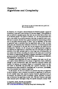
Haynes et al. [21] showed the NP-completeness of PDS by giving a reduction from 3-SAT. This also gives that PDS remains NP-complete when the input graph is bipartite or chordal. As DS is the same as PDS without applying OR2, a natural question arises: does OR2 make PDS more difficult to solve than DS? Intuitively, one would say yes due to the non-locality of this rule. In this section, we give some first evidence for this intuition, that is, we show, for general graphs, that PDS is at least as hard to solve as DS by reducing DS to PDS. We remark that our reduction from DS to PDS is much simpler than the one from 3-SAT to PDS. Moreover, our reduction implies the NP-completeness of PDS also in case of bipartite, chordal, circle, and planar graphs. Polynomialtime inapproximability and parameterized intractability results for DS transfer to PDS along the same lines. Theorem 1. Power Dominating Set is NP-complete in bipartite, chordal, circle, and planar graphs. Proof. Since it can be easily decided whether a vertex set P is a power dominating set, PDS is in NP. To show NP-hardness, we give a reduction from DS. Given a DS-instance with G = (V, E) and the parameter k, we construct a PDS-instance with G0 = (V ∪ V1 , E ∪ E1 ) and the same parameter k: attach newly introduced degree-one vertices to all vertices from V . Figure 1 illustrates this transformation. Let D be a dominating set of G. We show that D is a power dominating set of G0 . By definition, all vertices from V are observed by OR1. Applying OR2 to every vertex in V , the vertices in V1 become observed as well. Thus, D is a power dominating set of G0 . 6

G0

G

Figure 1: An example of the reduction from DS to PDS in the proof of Theorem 1. The vertices in V1 are drawn white. If G0 has a power dominating set P , then we can assume due to Lemma 1 that each vertex of P has degree at least three. This implies that P ∩ V1 = ∅. In order to observe a vertex v ∈ V1 , OR1 or OR2 has to be applied to v’s only neighbor u ∈ V . This means that either u ∈ P or u’s neighbors in G cannot be observed by applying OR2 to u. Hence the vertices in V \P must be observed by applying OR1 to one of their neighbors in G. This means that P is a dominating set for G. It is easy to verify that the reduction preserves the graph properties “bipartite,” “chordal,” “circle,” and “planar.” Hence, the NP-completeness of PDS follows from the NP-completeness of DS for bipartite graphs [14], chordal graphs [10], circle graphs [25], and planar graphs [19]. The reduction in the proof of Theorem 1 was independently achieved by Kneis et al. [27]. Observe that it is a gap-preserving as well as a parameterized reduction. This implies that all negative results with respect to the approximability and parameterized tractability with respect to the solution size for DS also are valid for PDS. As a consequence, it is hard to polynomial-time approximate PDS better than Θ(log |V |) [17] and PDS is W[2]-hard with the size of the power dominating set as parameter [16]. Next, we show that PDS is NP-complete in split graphs.4 The reduction is from the NP-complete Vertex Cover problem [19]: Given an undirected graph G = (V, E) and an integer k ≥ 0, is there a set C ⊆ V with |C| ≤ k such that each edge has at least one endpoint in C? Theorem 2. Power Dominating Set is NP-complete in split graphs. Proof. For a Vertex Cover instance with graph G = (V, E), we construct a split graph G0 from G as follows. For each edge e = {u, v} ∈ E we add a new vertex we and two edges between we and u and between we and v to G. We denote the set of the vertices we by VE . Moreover, we introduce for each vertex v ∈ V a new degree-one vertex v 0 and an edge between v and v 0 . The set 4 A reduction from 3SAT to PDS in split graphs has been described by Liao and Lee [29]. Note that the reduction given in the proof of Theorem 2 is a gap-preserving reduction. This implies that PDS is MaxSNP-hard in split graphs which does not follow from the previous results [29].

7

G

G0

Figure 2: An example of the reduction from Vertex Cover to PDS in the proof of Theorem 2. The vertices in VE and V1 are drawn grey and white, respectively. of these vertices is denoted by V1 . Finally, we complete the graph induced by V into a clique. Note that the subgraph of G0 induced by the vertices in VE ∪ V1 is an independent set. Thus, G0 is a split graph. See Figure 2 for an example. We claim that G has a vertex cover of size k iff G0 has a power dominating set of size k. The proof of the claim uses a similar argument as in the proof of Theorem 1 [31]. In summary, Table 1 compares the computational complexity of PDS and DS. By means of Theorems 1 and 2 we now have established NP-completeness results for PDS on all graph classes where NP-completeness is listed for DS by Kratsch [28].5 Liao and Lee [29] showed that PDS is polynomial-time solvable in interval graphs.

4

Dynamic Program for Graphs of Bounded Treewidth

We have seen in the previous section that PDS is W[2]-hard with respect to the parameter k denoting the size of the power dominating set. This means that, in general, there is basically no hope for an algorithm solving PDS in f (k) · nO(1) time, that is, restricting the combinatorial explosion only to the parameter k (herein, f (k) is a computable function only depending on the parameter k and may be exponentially growing or even worse). By way of contrast, only trivial nO(k) algorithms seem feasible for PDS. Hence, the natural question arises whether we can restrict the combinatorial explosion to other useful parameters. In fact, we show here that we can do so. More specifically, we show that PDS can be solved in f (k) · n time when k denotes the treewidth of the underlying graph. In other words, PDS is fixed-parameter tractable with respect to treewidth. Our main result in the following is to show that, when given a tree decomposition of bounded width for the underlying graph, PDS can be solved in linear time. To this end, we develop a concrete dynamic program using tree decompositions of graphs (Section 4.2). Before that, we start with the simple 5 Note that the class of comparability graphs is a superclass of the class of bipartite graphs [11]. The NP-completeness of PDS for this graph class directly follows from the NP-completeness of PDS for bipartite graphs.

8

Table 1: The first column is taken from Kratsch [28]. Partial k-trees are the same as graphs of treewidth k; the linear-time result for partial k-trees with fixed k is shown in Section 4. The result for interval graphs is due to Liao and Lee [29]. Empty entries mean that this has not been studied yet. Graph classes Dominating Set Power Dominating Set bipartite chordal circle comparability planar split AT-free cocomparability distance hereditary dually chordal interval k-polygon (k ≥ 3) partial k-tree (k ≥ 1) permutation strongly chordal

NP-complete NP-complete NP-complete NP-complete NP-complete NP-complete poly. time poly. time poly. time linear time poly. time poly. time linear time linear time poly. time

NP-complete NP-complete NP-complete NP-complete NP-complete NP-complete

poly. time linear time

special case of trees (Section 4.1). These results improve previous results from the literature [21, 27].

4.1

Trees

Haynes et al. [21] gave a linear-time algorithm for PDS in trees. As a warm-up for our algorithm working on graphs of bounded treewidth, we start with a much simpler linear-time algorithm for these “treewidth-one graphs.” Without loss of generality, we assume that the input tree T is rooted at a degree-one vertex r and the depth of a vertex v is defined as the length of the path between v and r. The algorithm follows a bottom-up strategy, see Figure 3. Theorem 3. Algorithm PDS-Trees from Figure 3 solves Power Dominating Set in trees in linear time. Proof. First, we prove that the output P of Algorithm PDS-Trees is a power dominating set. The proof is based on an induction on the depth of the vertices u in T , denoted by depth(u). Note that the proof works top-down whereas the algorithm works bottom-up. For depth(u) = 0, it is clear that u which is r is observed due to the “if”-condition on line 9 of Algorithm PDS-Trees. Suppose that all vertices u with depth(u) < k with k > 0 are observed. Consider a vertex u with depth(u) = k which is a child of the vertex v. If v ∈ P , then u is observed; otherwise, due to the induction hypothesis, v is observed. 9

1 2 3 4 5 6 7 8 9 10 11 12

PDS-Trees Input: Rooted tree T with r denoting the root Output: Minimum power dominating set P Sort the inner nodes of T in a list L according to a post-order traversal of T ; while L 6= {r} do v ← the first node in L; L ← L \ {v}; if v has at least two unobserved children then P ← P ∪ {v}; Exhaustively apply the two observation rules to T ; end if end while if r is unobserved then P ← P ∪ {r}; end if return P

Figure 3: Algorithm to compute a minimum power dominating set of a tree. Moreover, if depth(v) ≥ 1, then v’s parent is observed as well. Because of the “if”-condition on line 4 of Algorithm PDS-Trees, v is not in P only if v has at most one unobserved child during the “while”-loop (line 2) of Algorithm PDSTrees processing v. If vertex u is this only unobserved child, then it gets observed by applying OR2 to v, because v itself and all its neighbors (including v’s parent and its children) with the only exception of u are observed by the vertices in P . In summary, we conclude that all vertices in T are observed by P . Next, we prove the optimality of P by showing a more general statement: Claim. Given a rooted tree T = (V, E) with root r, Algorithm PDS-Trees outputs a power dominating set P such that |P ∩ Vu | ≤ |Q ∩ Vu | for any optimal solution Q of PDS for T and any tree vertex u, where Vu denotes the vertex set of the subtree of T rooted at u. Proof of the Claim. We use Tu = (Vu , Eu ) to denote the subtree of T rooted at vertex u. Let l denote the depth of T , that is, l := maxv∈V {depth(v)}. For each vertex u ∈ V , we define pu := |P ∩ Vu | and qu := |Q ∩ Vu |. We use an induction on the depth of tree vertices to prove the claim, starting with the maximum depth l and proceeding to 0. Since vertices u with depth(u) = l are leaves and Algorithm PDS-Trees adds no leaf to P , then we have pu = 0 and thus pu ≤ qu for all u with depth(u) = l. Suppose that pu ≤ qu holds for all u with depth(u) > k with k < l. Consider a vertex u with depth(u) = k. Let Cu denote the set of u’s children. Then, for all v ∈ Cu , by the induction hypothesis, we have pv ≤ qv . In order to

10

show pu ≤ qu , we only have to consider the case that X X qv . pv = (a) u ∈ P, (b) u ∈ / Q, and (c) v∈Cu

(1)

v∈Cu

In all other cases, pu ≤ qu always holds. In the following, we will show that this case does not apply. We assume that u 6= r. The argument works also for u = r. From (c) and, for all v ∈ Cu , pv ≤ qv (induction hypothesis), we know that pv = qv for all v ∈ Cu . Moreover, (a) is true only if u has two unobserved children v1 and v2 during the “while”-loop of Algorithm PDS-Trees processing u (the “if”-condition on line 4). In other words, this means that vertices v1 and v2 are not observed by the vertices in (P ∩ Vu ) \ {u}. In the following, we show that u has to be included in Q in order for Q to be a valid power dominating set. To this end, we need the following: ∀ x ∈ (Q ∩ Vvi ), 1 ≤ i ≤ 2 : ∃x0 ∈ W(vi ,x) : x0 ∈ P

(2)

where W(vi ,x) denotes the path between vi and x (including vi and x). Without loss of generality we consider only i = 1. Assume that predicate (2) is not true for a vertex x ∈ Q ∩ Vv1 . Since x ∈ / P , we can infer that px < qx . Since no vertex from W(v1 ,x) is in P and, by induction hypothesis, py ≤ qy for all y ∈ Vv1 , it follows that px0 < qx0 for all vertices x0 ∈ W(v1 ,x) , in particular, pv1 < qv1 . This contradicts the fact that pvi = qvi for all of u’s children vi . Thus, we have shown that predicate (2) is true. By predicate (2), for each vertex x ∈ Q ∩ Vvi (i ∈ {1, 2}), there exists a vertex x0 ∈ P on the path W(vi ,x) . Thus, if vertex vi is observed by a vertex x ∈ Q ∩ Vvi , then there is a vertex x0 ∈ P ∩ W(vi ,x) that observes vi . However, (a) in (1) is true only if v1 and v2 are unobserved by the vertices in P ∩ Vv1 and P ∩ Vv2 . Altogether, this implies that v1 and v2 cannot be observed by the vertices in Q ∩ Vv1 and Q ∩ Vv2 . Since Q is a solution for PDS in T , we have to take u into Q; otherwise, u has two unobserved neighbors v1 and v2 . OR2 can never be applied to u whatever vertices P from V \ Vu are P in Q. We can conclude that the case that u ∈ P , u ∈ / Q, and v∈Cu pv = v∈Cu qv does not apply. This completes the proof of the claim. Concerning the running time, we explain how to implement the exhaustive application of OR1 and OR2 (line 6 in Figure 3). Observe that, if OR2 is applicable to a vertex u during the bottom-up process, then all vertices in Tu can be observed at the current stage of the bottom-up process. In particular, after adding vertex u to P , all vertices in Tu can be observed. Thus, exhaustive application of OR1 and OR2 to the vertices of Tu can be implemented as pruning Tu from T which can be done in constant time. Next, consider the vertices in V \ Vu . After adding u to P , the only possible application of OR1 is that u observes u’s parent v. Moreover, we check the applicability of OR2 to the vertices x lying on the path from u to r, in the order of their appearance, the first v, and the last r. As long as OR2 is applicable to a vertex x on this path, we delete x from the list L that is defined in line 1 of Algorithm PDS-Trees, and prune Tx from T . 11

The linear running time of the algorithm is then easy to see: The vertices to which OR2 is applied are removed from the list L immediately after the application of OR2 and are never processed by the instruction in line 3 inside the “while”-loop (Figure 3). With proper data structures such as integer counters storing the number of observed neighbors of a vertex, the application of the observation rules to a single vertex can be done in constant time. Post-order traversal of a rooted tree is clearly doable in linear time.

4.2

Graphs of Bounded Treewidth

Our linear-time algorithm for graphs of bounded treewidth—assuming that the corresponding tree decomposition is given—uses basically the same strategy as the algorithms for DS [33, 34, 3, 6], that is, bottom-up dynamic programming from the leaves to the root. In the following, we demonstrate that there are two difficulties associated with OR2 that make PDS “harder” than DS and which cannot be solved by a simple modification of the algorithms for DS. First, with OR2, there are more possibilities for a vertex to be observed. More precisely, the application of OR2 implies that there is a certain “observation dependency” between two vertices, that is, one vertex not in the power dominating set that becomes observed can make one of its neighbors observed. This observation dependency does not exist in DS. There, the domination status of one vertex that is not in the dominating set has no effect on the domination status of other vertices. Therefore, in order to describe this observation dependency in the dynamic programming, the three states defined in the algorithms for DS for the vertices in a bag, namely, “belonging to the dominating set,” “already dominated at the current bag,” and “not yet dominated at the current bag,” are not sufficient. Second, only introducing further vertex states cannot settle the problem with the observation dependency. For example, assume that one defines the following additional state for the vertices in a bag: “already observed at the current bag by applying OR2 to one of its neighbors.” Then, there could emerge a “cycle of observation dependencies” as follows: Considering a simple cycle as the input graph, one might assign the new state “observed due to OR2” to each vertex of the cycle. This is “locally correct” but globally it is false because the reasoning is done in a circular fashion without “global justification.” Our answer to these two difficulties is to define, in addition to the vertex states, three states for the edges in the subgraph induced by the vertices in a bag. In fact, these states give one of three possible orientations to an undirected edge {u, v}, orienting it from u to v, orienting it from v to u, or leaving it unoriented. These orientations express observation dependencies. 4.2.1

Valid Orientations of Undirected Graphs

In the following, we define the orientations. Definition 4. An orientation of an undirected graph G = (V, E) is a graph D = ˙ 2 ) such that, for each {u, v} ∈ E, there is either a directed edge (u, v) (V, E1 ∪E 12

or (v, u) in E1 or an undirected edge {u, v} in E2 . The indegree of a vertex v in D, denoted by d− (v), is defined as |{(u, v) : (u, v) ∈ E1 }| and the outdegree of v, denoted by d+ (v), as |{(v, u) : (v, u) ∈ E1 }|. The subgraph D[V 0 ] induced by V 0 ⊆ V in D is called a suborientation. Note that in the standard graph theory literature, an orientation of an undirected graph G is a directed graph D where there is exactly one of (u, v) and (v, u) in D for each edge {u, v} in G. Here, we abuse the term orientation to denote a graph that results from orienting only a subset of edges. A directed edge (u, v) is called an outgoing edge for u and an incoming edge for v. Definition 5. A dependency path in an orientation D = (V, E1 ∪ E2 ) is a subgraph of D consisting of a sequence of vertices and edges v1 , e1 , v2 , e2 , . . . , ei−1 , vi with i ≥ 3, satisfying: 1. for all 1 ≤ j, k ≤ i, vj = vk ⇔ j = k, 2. for all 1 ≤ j ≤ i − 1, either ej = (vj , vj+1 ) ∈ E1 or ej = {vj , vj+1 } ∈ E2 , 3. and for all 1 ≤ j ≤ i − 1, at least one of ej and ej+1 is from E1 . The vertices v1 and vi are called the tail endpoint and the head endpoint of the dependency path, respectively. A dependency cycle in an orientation is a dependency path with an edge between vi and v1 which can be undirected only if (v1 , v2 ) ∈ E1 and (vi−1 , vi ) ∈ E1 ; otherwise, it is directed. A directed path is a dependency path with only directed edges. Observe that a dependency path contains at least one directed edge. Definition 6. A valid orientation D = (V, E1 ∪E2 ) of an undirected graph G = (V, E) is an orientation such that 1. ∀v ∈ V : (d− (v) ≤ 1) and (d− (v) = 1 ⇒ d+ (v) ≤ 1), 2. and there is no dependency cycle in D. We call the set of vertices with d− (v) = 0 the origin of D. Note that each graph is a valid orientation of itself. See Figure 4 for an example of a valid orientation. Note that one can decide in O(|E1 ∪ E2 |) time by depth-first search whether an orientation D is valid and, if so, find the origin of D. The following lemma is also easy to show. Lemma 4. Let D = (V, E1 ∪ E2 ) denote a valid orientation of an undirected graph G with origin O ⊆ V . 1. For each vertex v ∈ V \ O, there is exactly one directed path from the vertices in O to v. 2. Two directed paths from O to two vertices in V \ O are vertex-disjoint with the possible exception of their tail endpoints in O. 13

D

G

Figure 4: An example of a valid orientation D of an undirected graph G. The origin O of D contains only one vertex, marked with a rectangular box. Proof. (1) First, we show that there is at least one directed path from a vertex in O to v ∈ / O. By Definition 6 we have d− (v) = 1 with (u, v) denoting this edge. If u ∈ O, then edge (u, v) is the desired path; otherwise, u ∈ / O and d− (u) = 1. Again, we apply the above argument to u. Since graph G contains a finite number of vertices and there is no dependency cycle, there has to be a vertex x ∈ O with a directed path from x to v. We denote this path as W . The uniqueness of path W follows from the fact that, with the only exception of the tail in O, each vertex on this path has an indegree of exactly one. (2) A directed path from a vertex in O to a vertex in V \ O cannot pass through a vertex in O due to Definition 6. Two directed paths crossing at a vertex u ∈ V \ O would imply d− (u) > 1 or d+ (u) > 1 which is not allowed by Definition 6. This completes the proof. With the notations given above, we can introduce the following central orientation problem. Valid Orientation with Minimum Origin (VOMO) Input: An undirected graph G = (V, E) and an integer k ≥ 0. Question: Is there a vertex subset O ⊆ V with |O| ≤ k such that G has a valid orientation with O as origin? The following theorem shows that this orientation problem is a reformulation of PDS. This new problem formulation will be a decisive technical tool for our dynamic programming strategy to be described in Section 4.2.2. Theorem 4. An undirected graph G has a power dominating set P iff G has a valid orientation with P as origin. Proof. “⇐”: Having a valid orientation D of G with O ⊆ V as the origin, we show by contradiction that O is a power dominating set of G. See Figure 5 for an illustration. Suppose that O is not a power dominating set. Then, there is a vertex v ∈ (V \ O) which is not observed by O. Since D is a valid orientation, there is a directed path p1 from a vertex in O to v (Lemma 4). Assume without loss of generality that v is the first unobserved vertex on p1 . Let u denote the predecessor of v on p1 . Vertex u cannot be in O; otherwise v would be observed 14

w

v

x

u

y

O

p1

z

p2

p3

Figure 5: An example illustrating the proof of “⇐” of Theorem 4. Here, we assume that a dependency cycle is already built using three directed paths. by OR1. Since u is observed and OR2 cannot be applied to u to observe v, there is another neighbor of u, denoted by w, which is not observed by O. Moreover, there is also a directed path p2 in D from a vertex in O to w. Due to Lemma 4, p1 and p2 should be vertex-disjoint with the possible exception of their tail endpoints in O. Let x denote the first unobserved vertex on p2 . By applying the above argument now to x, vertex y which is x’s predecessor on p2 has an unobserved neighbor z 6= x and there is a directed path p3 from a vertex in O to z. Paths p1 , p2 , and p3 are pairwise vertex-disjoint ignoring their tail endpoints in O. We apply this argument further to the first unobserved vertex on p3 and so on. Since V is finite, we will encounter a vertex on one of the already considered paths p1 , p2 , p3 , . . . and, then, there exists a dependency cycle in D. This is a contradiction to the fact that D is a valid orientation. “⇒”: We prove this direction by describing a process which, for a given undirected graph G = (V, E) with a power dominating set P , constructs a valid orientation D of G with P as origin. Let V 0 := V and Vo := ∅. The process simulates the applications of OR1 and OR2 and moves the vertices from V 0 to Vo . The sets V 0 and Vo store the unobserved and the observed vertices, respectively. For each vertex v ∈ V \ P , the process directs exactly one of the edges incident to v. An integer c counting the rounds of moves is initialized to zero and will be increased by one for each vertex moving from V 0 to Vo . In addition, the process records the number of the round when vertex v is moved from V 0 to Vo in an integer variable tv ; the value of tv is set to the current value of c when moving v. At the beginning, all vertices from P are moved from V 0 to Vo in an arbitrary order. Note that the count c increases continuously and variables tv are set for each moved vertex v. Then, the process considers vertices v ∈ V 0 which satisfy the following condition: (?) v ∈ N (u) for the vertex u ∈ P which has the minimum tu among all vertices w ∈ P with V 0 ∩ N (w) 6= ∅. 15

The process moves vertex v from V 0 to Vo and edge (u, v) is inserted into E1 . This operation is executed for all vertices in V 0 ∩ N (P ). Note that now all applications of OR1 are simulated and Vo contains the vertices observed by OR1. After that, if V 0 is not empty, then all vertices in V 0 have to be observed by OR2. Since P is a power dominating set, as long as V 0 is non-empty the process can always find a vertex v ∈ V 0 which satisfies the following condition: (??) v ∈ N (u) where u ∈ Vo with (N [u] \ {v}) ⊆ Vo . Then, edge (u, v) is added to E1 and V 0 := V 0 \ {v} and Vo := Vo ∪ {v}. After repeatedly applying this operation to each vertex in V 0 , all edges in E which have no corresponding directed edges in E1 are added to E2 and D := (V, E1 ∪ E2 ). It is obvious that this process terminates after |V | rounds because P is a power dominating set of G. In the following, we prove that D is a valid orientation with P as origin. It is clear that D is an orientation. In the process described above, we can also observe that d− (v) = 0 for all v ∈ P and a vertex is removed from V 0 only if it has received an incoming edge in E1 . Hence, we have P = {v ∈ V : d− (v) = 0}. The first condition in the definition of valid orientations (Definition 6) is clearly satisfied by D: The vertices in P have no incoming edge and, because of (?), every vertex u ∈ N (P ) has exactly one incoming edge from a vertex v ∈ N (u)∩P which has the minimum tv among all vertices in N (u)∩P . A vertex u ∈ V \(P ∪N (P )) is moved from V 0 to Vo immediately after one of u’s incident edges is directed to u. Thus, for all vertices v ∈ V , it holds d− (v) ≤ 1. Moreover, if a vertex u with d− (u) = 1 has an outgoing edge (u, v), then u ∈ / P , vertex v is observed by applying OR2 to u, and v ∈ / P ∪ N (P ). Since, by (??), the process adds edge (u, v) to E1 for a vertex v ∈ V \ (P ∪ N (P )) only if (N [u] \ {v}) ⊆ Vo , the edge (u, v) is the only directed edge outgoing from u. Therefore, we obtain that d+ (v) ≤ 1 for all vertices v ∈ V with d− (v) = 1. It remains to show that there is no dependency cycle in D. Suppose that there is a dependency cycle in D and we order the vertices of this cycle v0 , v1 , v2 , . . . , vi with i > 2 and v0 = vi according to their appearance on the cycle. To simplify the presentation, we assume that vj = vj mod i . We show that no vertex from P can be on this cycle: Suppose that this dependency cycle contains a vertex of P , that is, vj ∈ P with 0 ≤ j < i. The edge between vj−1 and vj has to be undirected, since the process directs no edge to a vertex in P . Obviously, the edge between vj−2 and vj−1 has to be a directed edge, (vj−2 , vj−1 ) ∈ E1 . Since a vertex from P has no incoming edge, we have vj−1 ∈ / P . As described above, the process firstly moves vertices in P from V 0 to Vo , then vertices in N (P ), and then vertices in V \ (P ∪ N (P )). Since vj−1 ∈ N (vj ) ⊆ N (P ) and (vj−2 , vj−1 ) ∈ E1 , it can be deduced that vj−2 ∈ P . Because of (?) we can also infer tvj−2 < tvj . Then, we apply the above argument for vj again to vj−2 and can conclude that vj−4 ∈ P and tvj−4 < tvj−2 . By applying the same argument to vj−4 and further vertices, we would have tvj < tvj and, thus, the dependency cycle cannot contain vertices from P . 16

Hence, the dependency cycle only consists of vertices from V \ P and the directed edges on this cycle represent the applications of OR2. If the edge between vj and vj+1 is a directed edge, then tvj+1 > tvj : The process gives tvj+1 a value greater than tvj after adding (vj , vj+1 ) to E1 . If the edge between vj and vj+1 is an undirected edge, then (vj+1 , vj+2 ) ∈ E1 (the third point in Definition 5). Because of (??), vj+2 can be moved from V 0 to Vo and edge (vj+1 , vj+2 ) can be added to E1 only if all vertices in N [vj+1 ] \ {vj+2 } are already moved from V 0 to Vo . Thus, we know tvj < tvj+2 . By applying this argument again and again to all directed and undirected edges in a cyclic fashion, we will get tvj > tvj . Hence, there is no dependency cycle and D is a valid orientation with P as the origin. With VOMO and Theorem 4, we have an alternative formulation of PDS. The advantage of VOMO is that, by orienting undirected edges, a dependency cycle, which corresponds to a cycle of observation dependencies in the power domination context, can be easily detected in the dynamic programming on the tree decomposition. 4.2.2

Dynamic Programming on Tree Decompositions

In what follows, we describe a dynamic programming procedure solving VOMO on graphs of bounded treewidth. As a consequence of Theorem 4, we thus also arrive at a solution for PDS. Given an undirected, connected graph G = (V, E) with V := {v1 , v2 , . . . , vn } and a nice tree decomposition h{Xi : i ∈ I}, T i of G with treewidth k, let Ti denote the subtree of T rooted at node i and let Gi denote S the subgraph of G induced by the vertices in the bags of Ti , that is, Gi := G[ j∈V (Ti ) Xj ]. FurS thermore, we use Yi to denote ( j∈V (Ti ) Xj ) \ Xi . Definition of states: During a bottom-up process our dynamic programming algorithm computes for every bag Xi the possible valid orientations of the subgraph Gi and stores the sizes of the origins of the valid orientations. Herein, the valid orientations of Gi are characterized by the bag states. A bag state s of a bag Xi is a combination of the states for all ordered pairs of vertices in Xi , the states of all vertices in Xi , and the states of the edges in G[Xi ]. Next, we will define the states for vertex pairs, for vertices, and for edges, respectively. Herein, we use s(uv), s(v), and s(e) to denote the state of an ordered pair of vertices u ∈ Xi and v ∈ Xi , the state of a vertex v ∈ Xi , and the state of an edge e ∈ E(G[Xi ]). The decisive point in the dynamic programming is to detect the dependency cycles in all possible orientations Di for Gi when reaching bag Xi . The dependency cycles inside suborientations Di [Xi ] can be detected by exhaustive search in Di [Xi ] which consists of at most k vertices. However, for each pair of vertices u and v in Xi with u 6= v, the detection of dependency cycles passing through some vertices in Yi is more involved. Such cycles consists of several dependency paths, some lying in Di [Xi ] and others lying completely in Di [Yi ].

17

v

u

Type 2

Type 1

v

u

v

u

v

u

Type 3

Type 4

Figure 6: The four dependency path types from Definition 7. By storing information about all dependency paths between all pairs of vertices u, v ∈ Xi that, with the exception of u and v, only pass through vertices in Yi , we will be able to detect all corresponding dependency cycles by exhaustive search in O(k!) time. More specifically, we define for each pair of vertices in Xi several states reflecting the information about such dependency paths. Herein, let V (p) be the set of the vertices on a dependency path p. We use puv to denote a dependency path with u and v as the tail and the head endpoint, respectively. The path puv is called a dependency path from u to v. Definition 7. There are four types of dependency paths puv from u to v in an orientation D: • Type 1: The first edge (between u and its successor on puv ) as well as the last edge (between v and its predecessor on puv ) of puv are directed edges. • Type 2: The first edge of puv is a directed edge but the last edge is undirected. • Type 3: The last edge of puv is a directed edge but the first edge is undirected. • Type 4: Both the first edge and the last edge of puv are undirected edges. In addition, the function g maps a dependency path p to one of the four types, that is, g(p) ∈ {Type 1, Type 2, Type 3, Type 4}. Figure 6 illustrates the four path types. Observe that, if there are two dependency paths puv and pvu in a valid orientation D, then g(puv ) 6= Type 1 and g(pvu ) 6= Type 1, and at least one of puv and pvu is Type 4 or one is Type 2 and the other is Type 3; otherwise, there is a dependency cycle in the suborientation D[V (puv ) ∪ V (pvu )] which we call a “path type conflict.” The states for an ordered vertex pair uv with u 6= v in Xi are defined according to the possible types of dependency paths from u to v in Di [Yi ∪ {u, v}]: There are 16 states for an ordered vertex pair uv according to the 16 possible subsets 18

s(v) = 1

s(v) = 2

s(v) = 3

s(v) = 4

s(v) = 5

Figure 7: The five states of a vertex v in a bag. of {Type 1, Type 2, Type 3, Type 4}. Such a state means that there is at least one dependency path between the vertex pair of each path type contained in the subset. With these vertex pair states, we can simply detect a dependency cycle at a bag Xi : check, for every two vertices u and v in Xi , whether there exists a path type conflict between s(uv) and s(vu), or whether there is a dependency path from u to v (or from v to u) in Di [Xi ] whose type together with one type in s(vu) (or in s(uv)) builds a path type conflict. Next, we define five vertex states s(v) for every vertex v in a bag Xi (see Figure 7 for an illustration): • s(v) = 1: there is exactly one directed edge from a vertex in Yi to v and no directed edge from v to vertices in Yi ; • s(v) = 2: there is exactly one directed edge from a vertex in Yi to v and exactly one directed edge from v to a vertex in Yi ; • s(v) = 3: there is no directed edge between v and the vertices in Yi ; • s(v) = 4: there are at least two directed edges from v to the vertices in Yi and there is no directed edge from the vertices in Yi to v; • s(v) = 5: there is exactly one directed edge from v to a vertex in Yi and no directed edge from the vertices in Yi to v. Note that, by the definition of valid orientations, a vertex in a valid orientation cannot have more than one incoming edge and a vertex with N − (v) = 1 cannot have more than one outgoing edge. Hence, the above list covers all possible cases that need to be considered. Furthermore, we define three edge states s(e) for the edges e = {u, v} in G[Xi ]: • s(e) = uv: edge e is directed from u to v, • s(e) = vu: edge e is directed from v to u, and • s(e) = ⊥: edge e is undirected. As a consequence, for a bag Xi with |Xi | ≤ k, we have at most 16k(k−1) · 5 · 3k(k−1)/2 bag states. In the following, we say that a valid orientation D is under the restriction of a bag state s of the bag Xi if D satisfies the following conditions: k

19

• the orientations in D of the edges in G[Xi ] coincide with their states given by s, • for each ordered vertex pair uv with u ∈ Xi and v ∈ Xi , the types of the dependency paths from u to v in D[Yi ∪ {u, v}] coincide with s(uv), and • for each vertex v ∈ Xi , the orientations of the edges between v and the vertices in Yi coincide with s(v). In the bottom-up dynamic programming we use a mapping Ai for each bag Xi which stores, for each bag state s, the minimum size of the origins of all possible valid orientations of Gi under the restriction of s. Due to the following easy-to-prove lemma, in the computation of the values for Ai we do not count vertices v for the size of an origin with d− (v) = 0 and d+ (v) ≤ 1. Lemma 5. For a connected, undirected graph G = (V, E) with |V | > 2, there is always a valid orientation with a minimum origin O ⊆ V such that each vertex v ∈ O has in G at least two neighbors from V \ O which are not neighbors of other vertices in O. Proof. The claim follows directly from Lemma 2 and the equivalence between PDS and VOMO in Theorem 4. Now, we have defined the states for a bag in a nice tree decomposition and proceed with the description of our dynamic programming for VOMO, which consists of an “initialization” and an “update phase.” In the following, we use valid(G[Xi ], si ) to denote the procedure deciding whether the edge states si (e) of the edges e in G[Xi ] form a valid orientation of G[Xi ]. Since G[Xi ] contains at most k vertices, valid(G[Xi ], si ) needs at most O(k!) time. Procedure valid(G[Xi ], si ) returns true if si implies a valid orientation of G[Xi ]; otherwise, it returns false. Initialization: For each leaf node i with bag Xi of the tree decomposition T , we initialize Ai as follows. For each bag state si , we set Ai (si ) := +∞ if (∃v ∈ Xi : si (v) 6= 3)∨(∃uv : u ∈ Xi ∧v ∈ Xi ∧si (uv) 6= ∅)∨(valid(G[Xi ], si ) = false); and, otherwise, Ai (si ) :=|{v ∈ Xi : ∃e = {v, u} ∈ E(G[Xi ]), e0 = {v, w} ∈ E(G[Xi ]) with u 6= w ∧ si (e) = vu ∧ si (e0 ) = vw}|. By this initialization step, we make sure that only those bag states are taken into consideration where the edge states form a valid orientation. Also, since Yi = ∅, s(v) for each v ∈ Xi should be assigned the vertex state 3, that is, there is no directed edge between v and vertices in Yi , and s(uv) for each ordered vertex pair u ∈ Xi and v ∈ Xi should be assigned the vertex pair state ∅, that is, there is no dependency path from u to v in Di [Yi ∪ {u, v}]. Note that, due to Definition 6 and Lemma 5, as vertices in the origin we count only the vertices 20

in Xi which are the tails of at least two directed edges in the valid orientation formed by the edge states in si . Update phase: After the initialization, we visit the bags of the tree decomposition bottom-up from the leaves to the root, determining the corresponding mappings Ai in each step. For each bag state si of a bag Xi , the following needs to be done: 1. Check whether the edge states given by si form a valid orientation of G[Xi ]. 2. Compute the set S si of “with si compatible bag states” sj (or “with si compatible bag state pairs” sj and sl for join nodes) of a child bag Xj (or two child bags Xj and Xl for join nodes). The formal definition of compatible bag states (and compatible bag state pairs) will be given individually for forget, insert, and join nodes, respectively (see the Appendix). 3. For a node i with a child node j, if Gi contains more edges than Gj , then, for each compatible bag state sj (or each compatible bag state pair) in S si , check whether a valid orientation of Gj under the restriction of sj can be extended to a valid orientation for Gi under the restriction of si , that is, whether a valid orientation for Gj under the restriction of sj combined with the orientations of the newly introduced edges in Gi which are given by si results in a valid orientation of Gi . For a node i with two children, the test whether the combination of two valid orientations is still a valid orientation of Gi can be carried out in a similar way. 4. Based on the mappings Aj for all compatible bag states (or bag state pairs) in S si , evaluate Ai (si ). The details of the dynamic programming are technical but use more or less standard methods. Hence, we defer these details into the Appendix. When reaching the root of T , we can determine the minimum size of the origin of a valid orientation of G in the mapping A of the root node. Altogether, we thus arrive at the following central result. Theorem 5. For an n-vertex graph with given width-k tree decomposition, 2 Valid Orientation with Minimum Origin can be solved in O(ck · n) time for a constant c. Proof. The correctness of the algorithm follows directly from the description (also see Appendix). Concerning the running time, the most time-consuming part of the algorithm is the determination of the mapping Ai for a join node, where, for each bag state, we have to examine all possible bag state pairs, one 2 2 from each child bag. As described above, there are less than 16k · 5k · 3k bag 2 2 states and, for each bag state s, there can be at most (16k · 5k · 3k )2 bag state pairs which are compatible to s. For each compatible bag state pair (sj , sl ), the dominating factor for the running time is to determine whether two valid orientations of Gj and Gl under the restrictions of sj and sl , respectively, can 21

be combined into a valid orientation of Gi under the restriction of si . This can be done in O(k!) time (see Appendix). In summary, this results in a worst-case 2 2 running time of O((16k · 5k · 3k )3 · k!) for a join node. Together with Theorem 4, we obtain our main result. Theorem 6. For an n-vertex graph with given width-k tree decomposition, 2 Power Dominating Set can be solved in O(ck · n) time for a constant c.

5

Conclusion

Besides improving the exponential worst-case complexity of our dynamic programming algorithm in Section 4, there are several avenues for future work. • Table 1 has several empty entries concerning the complexity of Power Dominating Set (PDS) in graph classes which we did not address here but have been addressed for Dominating Set (DS) [28]. In particular, is there a “significant” difference between the complexities of DS and PDS (also see the discussion in Section 1 and the very recent work of Aazami and Stilp [1])? • Which graph classes where PDS is NP-complete allow for better than factor-Θ(log n) polynomial-time approximation algorithms? • How do fixed-parameter tractability results for DS in planar graphs [3, 4, 5] transfer to PDS? • Are there nontrivial polynomial-time data reduction rules for PDS similar to those we have for DS [5]? • Are there further “distance from triviality” parameterizations [20] that make PDS algorithmically feasible? This paper particularly aims at stimulating a comparative study concerning the computational complexities of DS and PDS. So far, we are not aware of a graph class where DS is polynomial-time solvable and PDS is NP-complete or vice versa. In other words, the point is to better understand which role the second, non-local observation rule of PDS plays from an algorithmic viewpoint. We believe that PDS offers a promising field of research not only because of its practical importance but also because it allows for a compact problem formulation within which one can nicely study effects of non-locality by comparing the “local” DS with the “non-local” PDS problem. To understand this phenomenon in greater depth is a challenge for future research. Acknowledgement. We are grateful to two anonymous referees of Algorithmica for their constructive feedbacks. In particular, one of the referees pointed out how to simplify the proofs of Lemma 2 and Theorem 1.

22

References [1] A. Aazami and M. D. Stilp. Approximation algorithms and hardness for domination with propagation. In Proc. 10th APPROX/11th RANDOM, LNCS. Springer, 2007. To appear. 3, 22 [2] C. Adjih, P. Jacquet, and L. Viennot. Computing connected dominating sets with multipoint relays. Ad Hoc & Sensor Wireless Networks, 1(1– 2):27–39, 2005. 2 [3] J. Alber, H. L. Bodlaender, H. Fernau, T. Kloks, and R. Niedermeier. Fixed parameter algorithms for Dominating Set and related problems on planar graphs. Algorithmica, 33(4):461–493, 2002. 3, 12, 22 [4] J. Alber, H. Fan, M. R. Fellows, H. Fernau, R. Niedermeier, F. Rosamond, and U. Stege. A refined search tree technique for Dominating Set on planar graphs. Journal of Computer and System Sciences, 71(4):385–405, 2005. 22 [5] J. Alber, M. R. Fellows, and R. Niedermeier. Polynomial time data reduction for Dominating Set. Journal of the ACM, 51(3):363–384, 2004. 22 [6] J. Alber and R. Niedermeier. Improved tree decomposition based algorithms for domination-like problems. In Proc. 5th LATIN, volume 2286 of LNCS, pages 613–628. Springer, 2002. 12 [7] G. Ausiello, P. Crescenzi, G. Gambosi, V. Kann, A. Marchetti-Spaccamela, and M. Protasi. Complexity and Approximation — Combinatorial Optimization Problems and Their Approximability Properties. Springer, 1999. 2, 4 [8] H. L. Bodlaender. A partial k-arboretum of graphs with bounded treewidth. Theoretical Computer Science, 209:1–45, 1998. 5 [9] H. L. Bodlaender. Treewidth: Characterizations, applications, and computations. In Proc. 32nd WG, volume 4271 of LNCS, pages 1–14. Springer, 2006. 5 [10] K. S. Booth and J. H. Johnson. Dominating sets in chordal graphs. SIAM Journal on Computing, 11:191–199, 1982. 7 [11] A. Brandst¨ adt, V. B. Le, and J. P. Spinrad. Graph Classes: a Survey. SIAM Monographs on Discrete Mathematics and Applications, 1999. 6, 8 [12] D. J. Brueni and L. S. Heath. The PMU placement problem. SIAM Journal on Discrete Mathematics, 19(3):744–761, 2005. 2 [13] E. D. Demaine and M. Hajiaghayi. Bidimensionality: New connections between FPT algorithms and PTASs. In Proc. 16th SODA, pages 590–601. ACM/SIAM, 2005. 3 23

[14] A. K. Dewdney. Fast Turing reductions between problems in NP: chapter 4; reductions between NP-complete problems. Technical report, Department of Computer Science, University of Western Ontario, Canada, 1981. 7 [15] M. Dorfling and M. A. Henning. A note on power domination in grid graphs. Discrete Applied Mathematics, 154(6):1023–1027, 2006. 2 [16] R. G. Downey and M. R. Fellows. Parameterized Complexity. Springer, 1999. 2, 4, 7 [17] U. Feige. A threshold of ln n for approximating Set Cover. Journal of the ACM, 45(4):634–652, 1998. 2, 7 [18] J. Flum and M. Grohe. Parameterized Complexity Theory. Springer, 2006. 2, 4 [19] M. R. Garey and D. S. Johnson. Computers and Intractability: A Guide to the Theory of NP-Completeness. Freeman, 1979. 4, 7 [20] J. Guo, F. H¨ uffner, and R. Niedermeier. A structural view on parameterizing problems: distance from triviality. In Proc. 1st IWPEC, volume 3162 of LNCS, pages 162–173. Springer, 2004. 22 [21] T. W. Haynes, S. M. Hedetniemi, S. T. Hedetniemi, and M. A. Henning. Domination in graphs: applied to electric power networks. SIAM Journal on Discrete Mathematics, 15(4):519–529, 2002. 2, 3, 4, 6, 9 [22] T. W. Haynes, S. T. Hedetniemi, and P. J. Slater, editors. Domination in Graphs: Advanced Topics, volume 209 of Pure and Applied Mathematics. Marcel Dekker, 1998. 1 [23] T. W. Haynes, S. T. Hedetniemi, and P. J. Slater. Fundamentals of Domination in Graphs, volume 208 of Pure and Applied Mathematics. Marcel Dekker, 1998. 1 [24] T. W. Haynes and M. A. Henning. Domination in graphs. In J. L. Gross and J. Yellen, editors, Handbook of Graph Theory, pages 889–909. CRC Press, 2004. 1 [25] J. M. Keil. The complexity of domination problems in circle graphs. Discrete Applied Mathematics, 36:25–34, 1992. 7 [26] T. Kloks. Treewidth: Computations and Approximations, volume 842 of LNCS. Springer, 1994. 5, 6 [27] J. Kneis, D. M¨ olle, S. Richter, and P. Rossmanith. Parameterized power domination complexity. Information Processing Letters, 98(4):145–149, 2006. 2, 3, 4, 7, 9

24

[28] D. Kratsch. Algorithms. In T. W. Haynes, S. T. Hedetniemi, and P. J. Slater, editors, Domination in Graphs: Advanced Topics, pages 191–231. Marcel Dekker, 1998. 8, 9, 22 [29] C. S. Liao and D. T. Lee. Power dominating problem in graphs. In Proc. 11th COCOON, volume 3595 of LNCS, pages 818–828. Springer, 2005. 2, 3, 7, 8, 9 [30] R. Niedermeier. Invitation to Fixed-Parameter Algorithms. Oxford University Press, 2006. 2, 4 [31] D. Raible. Algorithms and Complexity Results for Power Domination in Networks (in German). Master’s thesis, Wilhelm-Schickard-Institut f¨ ur Informatik, Universit¨ at T¨ ubingen, Germany, 2005. 8 [32] B. A. Reed. Algorithmic aspects of tree width. In B. A. Reed and C. L. Sales, editors, Recent Advances in Algorithms and Combinatorics, pages 85–107. Springer, 2003. 5 [33] J. A. Telle and A. Proskurowski. Practical algorithms on partial k-trees with an application to domination-like problems. In Proc. 3rd WADS, volume 709 of LNCS, pages 610–621. Springer, 1993. 12 [34] J. A. Telle and A. Proskurowski. Algorithms for vertex partitioning problems on partial k-trees. SIAM Journal on Discrete Mathematics., 10(4):529–550, 1997. 12 [35] V. V. Vazirani. Approximation Algorithms. Springer, 2001. 2, 4

25

Appendix: Details of the dynamic programming. Forget Nodes: Suppose that node i is a forget node with child node j, that is, Xi := {xi1 , . . . , xini } and Xj := {xi1 , . . . , xini , x}. Since Gi and Gj contain the same set of edges, each valid orientation of Gj is also a valid orientation of Gi . For each bag state si of node i, we compute the set S si containing the bag states sj of node j that are compatible with si . Note that, if there exists an edge between a vertex v ∈ Xi and the vertex x, then the orientation of edge {v, x} can result in a difference between si (v) and sj (v). For example, a vertex with sj (v) = 4 having an edge {v, x} with sj ({v, x}) = vx should have si (v) = 5. The reason is that now vertex v has two outgoing edges to vertices in Yi , the new one being (v, x). Herein, we say that sj is compatible with si with respect to a vertex v ∈ Xi if one of the following is true: • si (v) = sj (v) ∧ ({x, v} ∈ / E ∨ ((e = {x, v} ∈ E) ∧ (sj (e) =⊥))), • sj (v) = 3 ∧ si (v) = 1 ∧ ((e = {x, v} ∈ E) ∧ (sj (e) = xv)), • sj (v) = 1 ∧ si (v) = 2 ∧ ((e = {x, v} ∈ E) ∧ (sj (e) = vx)), • sj (v) = 5 ∧ si (v) = 2 ∧ ((e = {x, v} ∈ E) ∧ (sj (e) = xv)), • sj (v) = 4 ∧ si (v) = 4 ∧ ((e = {x, v} ∈ E) ∧ (sj (e) = vx)), • sj (v) = 5 ∧ si (v) = 4 ∧ ((e = {x, v} ∈ E) ∧ (sj (e) = vx)), • sj (v) = 3 ∧ si (v) = 5 ∧ ((e = {x, v} ∈ E) ∧ (sj (e) = vx)). To define the compatibility of sj with respect to an ordered vertex pair, we introduce a so-called concatenation function of path types. This partial function maps two given path types to a path type. If the path resulting by identifying the head endpoint of a path of the first path type and the tail endpoint of a path of the second path type is a dependency path, then this function is defined and returns the type of the resulting path; otherwise, it is not defined. For example, if the first path type is Type 1 and the second is Type 2, then the function returns Type 2; if the first path type is Type 2 and the second is Type 3, the resulting path is not a dependency path and the concatenation function is not defined. We say that sj is compatible with si with respect to an ordered vertex pair uv with u ∈ Xi and v ∈ Xi if si (uv) extends sj (uv) by concatenating the path types in sj (ux) and the path types in sj (xv) and by adding the type of the possible dependency path from u to v formed by edges {u, x} and {v, x}. For example, if edges e = {u, x} and e0 = {v, x} are in E and sj (e) = ux and sj (e0 ) =⊥, then we have a Type-2-path from u to v passing through x. Hence, sj is compatible with si with respect to uv if sj (uv) = {Type 1, Type 4}, sj (ux) = ∅, sj (xv) = ∅, and si (uv) = {Type 1, Type 2, Type 4}. The bag states sj ∈ S si that are compatible with si have to satisfy the following conditions: 26

• for each e ∈ E(G[Xi ]), si (e) = sj (e), • sj is compatible with si with respect to each v ∈ Xi , and • sj is compatible with si with respect to each ordered vertex pair uv with u ∈ Xi and v ∈ Xi . Then, evaluate the mapping Ai of Xi as follows: For each bag state si , set Ai (si ) := mins {Aj (sj )}. sj ∈S

i

Note that, if S si = ∅ for an si , then Ai (si ) = +∞. The computation of Ai (si ) is correct since Gi and Gj have the same set of edges and, thus, each valid orientation of Gi is also a valid orientation of Gj . Introduce Nodes: Suppose that node i is an introduce node with child node j, that is Xi := {xj1 , . . . , xjnj , x} and Xj := {xj1 , . . . , xjnj }. Procedure valid(G[Xi ], si ) can decide whether the edge states contained in si form a valid orientation of G[Xi ] in O(k!) time. For each bag state si of node i, we compute the set S si containing the with si compatible bag states sj of node j which satisfy (∀e ∈ E(G[Xj ]) : si (e) = sj (e)) ∧ (∀v : si (v) = sj (v)) ∧ (∀uv : si (uv) = sj (uv)), where u, v ∈ Xj . Note that the introduction of a new vertex x does not change the number of directed edges between a vertex v ∈ Xj and the vertices in Yi ; thus, si (v) = sj (v). The types of the dependency paths remain the same for each ordered vertex pair uv with u ∈ Xj and v ∈ Xj , that is, si (uv) = sj (uv). Moreover, since there is no edge between the new vertex x ∈ Xi and the vertices in Yi (due to the consistency property of tree decompositions), we set S si := ∅ for bag states si where si (x) 6= 3 or where there is a vertex v ∈ Xj with si (vx) 6= ∅ or si (xv) 6= ∅. The next task is to decide whether a valid orientation of Gj under the restriction of a bag state sj ∈ S si can be extended to a valid orientation of Gi under the restriction of si . Herein, note that Gi has one more vertex x than Gj and, hence, we have to take into account the states of the edges incident to x in G[Xi ]. Observe that the conditions for a valid orientation can be violated by a vertex in N (x) ∩ Xi or by a dependency cycle passing through vertex x. First, for each vertex v in N (x)∩Xi , we can easily find out the indegree and outdegree of v in the orientation of Gj under the restriction of sj , based on the information stored in sj (v) and sj (e) for all edges e in E(Gj ) incident to v. Together with the orientation of edge e = {v, x} given by si (e), the indegree and outdegree of v in the orientation of Gi under the restriction of si can be easily determined. Hence, to check whether a vertex v ∈ N (x) ∩ Xi violates the vertex-degree conditions of a valid orientation, that is, d− (v) ≤ 1 and d− (v) = 1 ⇒ d+ (v) ≤ 1, can be done in O(k 2 ) time because there can be at most O(k 2 ) edges between vertices in Xj . Second, if there is a dependency cycle passing through x in the 27

orientation of Gi under the restriction of si , then it consists of some consecutive dependency paths between some pairs of the vertices in Xj and two edges incident on x. By accessing the information about the dependency path types stored in sj (vu) for each ordered vertex pair with u, v ∈ Xj , an exhaustive search running in O(k!) time can easily decide whether there are such dependency cycles. Altogether, we can in O(k!) time decide whether a valid orientation of Gj under the restriction of a bag state sj ∈ S si can be extended to a valid orientation of Gi under the restriction of si . If the valid orientation of Gj under the restriction of sj ∈ S si cannot be extended to a valid orientation of Gi under the restriction of si , then we remove sj from S si . Finally, we compute the mapping Ai (si ) for si based on the mappings Aj (sj ) for all sj ∈ S si . By orienting the edges which are incident to the new vertex x according to the edge states given by si , vertex x could have more than one outgoing edge. Moreover, the outdegrees of vertices v ∈ Xi which are adjacent to x and have outdegree one in the valid orientation of Gj under the restriction of sj could also become two. As a consequence, we should add x and those of x’s neighbors which now have outdegree two into the origin of the valid orientation of Gi under the restriction of si . Therefore, we introduce in the following two functions B and f to cope with these possible new origin vertices. The mapping Ai for Xi is computed as follows: For each bag state si , set Ai (si ) := mins {Aj (sj ) + fsi (x) + |Bsi (sj )|}, sj ∈S

i

where fsi (x) = 1 if there exist at least two edges e = {u, x} and e0 = {v, x} in G[Xi ] with si (e) = xu and si (e0 ) = xv; otherwise, fsi (x) = 0. The function Bsi (sj ) returns the set of vertices u ∈ (N (x) ∩ Xj ) which satisfy one of the following two conditions: • sj (u) = 5 and si ({u, x}) = ux or • sj (u) = 3, si ({u, x}) = ux, and si ({u, v}) = uv for an edge {u, v} ∈ E(G[Xi ]) with v 6= x. Roughly speaking, fsi (x) = 1 covers the case that x has to be added to the origin and the set returned by Bsi (sj ) contains the vertices which are in the origin of the valid orientation of Gi but not in the origin of the valid orientation of Gj . Note that, if S si = ∅ for a si , then Ai (si ) = +∞. Join Nodes: Suppose that i is a join node with child nodes j and l, that is Xi := {xi1 , . . . , xini } and Xi = Xj = Xl . The considerations for join nodes are almost the same as for forget and introduce nodes. There are two points to note here. Let S si be the set of the bag state pairs (sj , sl ) that are compatible with si . Note that, due to the consistency property of tree decompositions, Yj ∩ Yl = ∅. Because Yi = Yj ∪ Yl , the indegree (outdegree, respectively) of v in G[Yi ∪ {v}] is equal to the sum of the indegrees (outdegrees, respectively) of v in G[Yj ∪ {v}] and in G[Yl ∪ {v}]. For example, if sj (v) = 1 and sl (v) = 5, then v has an 28

incoming edge from a vertex in Yj and an outgoing edge to a vertex in Yl and, thus, si (v) = 2. Therefore, we say that si is compatible with sj and sl with respect to vertex v ∈ Xi if one of the following is true: • si (v) = 1 ∧ ((sj (v) = 1 ∧ sl (v) = 3) ∨ (sj (v) = 3 ∧ sl (v) = 1)), • si (v) = 2 ∧ ((sj (v) = 2 ∧ sl (v) = 3) ∨ (sj (v) = 3 ∧ sl (v) = 2) ∨ (sj (v) = 1 ∧ sl (v) = 5) ∨ (sj (v) = 5 ∧ sl (v) = 1)), • si (v) = 3 ∧ sj (v) = 3 ∧ sl (v) = 3, • si (v) = 4 ∧ ((sj (v) = 4 ∧ sl (v) = 3) ∨ (sj (v) = 3 ∧ sl (v) = 4) ∨ (sj (v) = 5 ∧ sl (v) = 5)), • si (v) = 5 ∧ ((sj (v) = 5 ∧ sl (v) = 3) ∨ (sj (v) = 3 ∧ sl (v) = 5)). With the fact that Yj ∩ Yl = ∅, a dependency path from vertex u ∈ Xi to vertex v ∈ Xi passing through vertices in Yj is then, with the exceptions of u and v, vertex-disjoint with any dependency path from u to v passing through vertices in Yl . Thus, the set of dependency paths from u to v passing through vertices in Yi is then the union of the set of dependency paths from u to v passing through vertices in Yj and the set of dependency paths from u to v passing through vertices in Yl . Therefore, we say that si is compatible with sj and sl with respect to an ordered vertex pair uv with u ∈ Xi and v ∈ Xi if si (uv) is the union of sj (uv) and sl (uv). In summary, the bag state pairs (sj , sl ) ∈ S si that are compitable with si satisfy the following conditions: • for each e ∈ E(G[Xi ]), si (e) = sj (e) = sl (e), • si is compatible with sj and sl with respect to each v ∈ Xi , and • si is compatible with sj and sl with respect to each ordered vertex pair uv with u ∈ Xi and v ∈ Xi . The next task is to check whether the combination of the two valid orientations of graph Gj and Gl which are under the restrictions of sj and sl , respectively, is a valid orientation of Gi under the restriction of si . This can be done in almost the same way as for the introduce nodes. The running time is O(k!). Finally, in order to compute the mapping Ai (si ) for a bag state si , observe that, by combining two valid orientations of Gj and Gl , there could emerge new origin vertices in the valid orientation of Gi . For example, a vertex v ∈ Xi has in each of the two valid orientations of Gj and Gl only one outgoing edge, one to a vertex in Yj and one to a vertex in Yl . Since Yi = Yj ∪ Yl , vertex v has now two outgoing edges in the valid orientation of Gi resulting from the combination of the valid orientations of Gj and Gl . The function B introduced below counts such new origin vertices. Moreover, there could be vertices in Xi which are in the origins of both valid orientations of Gj and Gl . Hence, by combining the 29

two valid orientations and summing up the size of the origins of the two valid orientations, there could be some vertices counted twice. In order to avoid such double counting we introduce a function C in the computation of Ai (si ). For each bag state si , the determination of Ai is done as follows: Ai (si ) :=

min

(sj ,sl )∈S si

{Aj (sj ) + Al (sl ) + |Bsi (sj , sl )| − |Csi (sj , sl )|},

where function Bsi (sj , sl ) returns the set of new origin vertices v ∈ Xi , that is, sj (v) = 5 and sl (v) = 5 and there is no edge e = {u, v} ∈ E(G[Xi ]) with si (e) = uv, and function Csi (sj , sl ) contains the vertices v ∈ Xi which satisfy one of the following conditions: • there are at least two edges e = {u, v}, e0 = {v, w} in E(G[Xi ]) with si (e) = vu and si (e0 ) = vw, • sj (v) = 5 and sl (v) = 5 and there is exactly one edge e = {u, v} in E(G[Xi ]) with si (e) = vu, or • sj (v) = 4 and sl (v) = 4.

30