Jun 21, 1983 - evoked potentials measured from five subjects. CONTINUOUS LCA. In order to use the LCA to make an improved estimate of the actual ERP ...
371
IEEE TRANSACTIONS ON BIOMEDICAL ENGINEERING, VOL. BME-32, NO. 6, JUNE 1985
Improved Waveform Estimation Procedures for Event-Related Potentials CLARE D. McGILLEM,
FELLOW, IEEE, AND CARLOS
Abstract-Several methods of estimating the waveform of eventrelated potentials are presented. The techniques of conventional averaging, Woody cross-correlation averaging, latency corrected averaging, continuous latency corrected averaging, and enhanced averaging are described and their results compared. It was found that the continuous latency corrected average appears to offer the most useful representation of the waveform of the event-related potential.
JORGE I. AUNON, A. POMALAZA
SENIOR MEMBER, IEEE,
peaks in the ERP. After the peaks have been detected, they are grouped according to the latencies at which they occurred. A sign test is then applied to the polarities of the peaks in small latency intervals to determine, with a high degree of confidence (typically 95 percent), those intervals in which the peaks present are different than would be produced by the ongoing EEG only. In this manner, the peaks belonging to the various component of the ERP are grouped together. The percentage of waveforms in which peaks are found corresponding to specific ERP components typically varies from around 20 percent to more than 90 percent of the waveforms contained in the ensemble. Short segments of the individual waveforms in the vicinity of the identified peaks are aligned so that the peaks coincide and the average of the aligned segments is computed. The resulting average for each segment is one component of the LCA. These components are plotted on a graph with each being located at the average latency of the peaks from which it was computed. Only short segments of the measured ERP's are used to form the LCA components. Since the subsets of ERP's used to form the different components are generally different, and the random variations of the latencies are removed, the components of the LCA are generally disjoint. Nevertheless, this type of presentation is very informative about the various components present and provides much more information than the conventional average. In order to provide a more conventional representation of the information contained in the LCA, a procedure has been developed to convert the disjoint segments of the LCA into a continuous waveform. This procedure is described in the next section and is called the continuous LCA. A different approach to recovering information lost in the averaging process is also described and leads to what is called the enhanced average. The results of applying all five of these procedures are illustrated for two sets of evoked potentials measured from five subjects.
INTRODUCTION THE most widely used estimator for event-related poItential (ERP) waveforms is the conventional average obtained as the sample mean of an ensemble of single ERP's timelocked to the instant of stimulus application. It is generally accepted that variations in the ERP waveform occur from one stimulus to the next and that these variations are lost by conventional averaging [4], [6], [10]. Several researchers have proposed techniques to recover some of the information lost by the averaging process. Two of these techniques are the Woody average [13] and the latency corrected average (LCA) 110], [3]. In the Woody procedure, the individual ERP waveforms are aligned to one another before averaging. The alignment is accomplished by finding the latency shift that gives a maximum cross-correlation coefficient between the waveforms and a template formed by the average of the previously aligned waveforms. Frequently, the procedure is repeated one or more times to obtain the final estimate. The Woody procedure is capable of compensating for shifts in latency of the entire waveform but cannot cope with random shifts of individual components of the ERP. Furthermore, if there are strong components such as alpha waves present, the Woody procedure may align to them [2]. Also, this procedure will lead to an apparent waveform enhancement when only the ongoing EEG is present, i.e., when no ERP has occurred. In an attempt to overcome the limitations of the Woody average, a technique called the latency corrected average (LCA) was developed [10]. In the LCA procedure, the individual components (peaks) in each ERP waveform are CONTINUOUS LCA first detected. This detection is aided by initially filtering the ERP's with a minimum mean-square error (MMSE) In order to use the LCA to make an improved estimate filter [1], [10], and then cross correlating the filtered wave- of the actual ERP waveshape, it is necessary to convert it forms with a template having the general shape of the into a smooth curve by an appropriate filtering procedure. Experiments were tried using a least-squares fitting of Manuscript received June 21, 1983; revised December 5, 1984. This work power series, Chebyshev polynomials, and Fourier series was supported by AFOSR Contract F83K0031. The authors are with the EEG Signal Processing Laboratory, School of (with the Fourier series giving the best results). In all cases Electrical Engineering, Purdue University, West Lafayette, IN 47907. the fit was excellent in regions where the LCA segments
0018-9294/85/0600-0371$01.00 © 1985 IEEE
IEEE TRANSACTIONS ON BIOMEDICAL ENGINEERING, VOL. BME-32, NO. 6, JUNE 1985
372
20.00
*0.00
-20.00
400.00 .00 LAT (MS)
600.00
0.00
40
200.00
LAT (MS)
Fig. 1. Superposition of the VEP conventional averages of low-pass filtered [30 Hz] data and their corresponding LCA's for two electrode positions. 40.00-
40.00
' 20.00
' 0.00
-40.00
0.00
0.60
0.00
SECS.
0.60
Fig. 2. Representation of the LCA's of Fig. were
Pz
located. However, when
one or more
I
0.20
with
a sum
SECS.
0.40
0.60
of sinusoids.
of the LU
components was missing (as is often the case), the
proximating function behaves erratically in the region the missing components. This is illustrated in Figs. 1 a 2. Fig. 1 shows the conventional average and LCA sup imposed for two sets of VEP's. Fig. 2 shows the U fitted by a sum of sinusoids. The large peaks in Fig occur where there are no components of the LCA pres and are obviously not a valid approximation in that regi In order to minimize such effects, a weighted least-squa fitting is used. The frequencies of the components are 9"§ lected first (the number of different frequencies possibli e is determined by the amount of data available), and then amplitudes of each component are determined. By elii nating those frequency components that have very sn nall coefficients and adding new components not previou isly used, an improved fit can be obtained by several itevrations. At the same time, by setting the values of the dlata in the vicinity of missing components equal to the conv,entional average and using a reduced weighting factor (1/ 10) in this region relative to the rest of the data set, the g eration of spurious peaks can be eliminated. The weighted least-squares fit is obtained as the solution to the maltrix equation a=[*-XTi-loTtor (1)
is the vector of coefficients of the expansion of the sinusoidal basis vectors, is a matrix where each of its row vectors are the different (discrete) basis vectors of the expansion, is the data vector being fitted, and is the vector weights, set according to the number of peaks found in each individual region of the LCA [see Fig. 4(c)].
The results of four iterations of the fitting procedure the continuous LCA waveforms shown in Fig. 3. Comparison of the continuous LCA waveforms to the disjoint LCA waveforms of Fig. 1 shows excellent agreement. A more detailed example of the computation of the continuous LCA of an ensemble of VEP's is illustrated in
gave
Table I and Fig. 4.
Table I shows the statistical results of applying the LCA procedure to an ensemble of VEP's (the actual experiment is described later under the Procedure section, and the data correspond to subject 3, lower checkerboard
stimulation).
Fig. 4(a) shows the LCA (solid) and the corresponding
ensemble average (dashed) for this experiment. Fig. 4(b)
373
MC GILLEM et al.: WAVEFORM ESTIMATION PROCEDURES FOR EVENT-RELATED POTENTIALS 20.0
>
00.0.
- 20.0
SECS.
SECS.
Fig. 3. Continuous LCA waveforms of Fig. 1 after four iterations of the representation procedure.
delay associated with each component. Let one of the components be s (t) and let n (t) be the noise occurring in the same latency interval as s (t). Then the measured sigAmplitude (MV) nal in this interval on the ith trial is ri(t) = s(t - r) + ni(t) (2) 6.4 4.1 where ri is a random variable representing the random la9.7 tency variation and having a probability density function (PDF) p (T). When a large number of responses are averaged, the conventional averaged ERP is obtained and is -3.2 -12.5 given by
TABLE I STATISTICS DETERMINED FROM THE LCA PROCEDURE
Peak
Range (ms)
Mean (ms)
1 2 3
68-100 128-164 188-240
76 147 209
1 2 3 4 5
44-68 96-136
53 112 169 246 315
S.D.
Percent
Positive Peaks 6 9 14
80
42 78
Negative Peaks
164-184
244-260 304-332
8 6 6 5 8
40
96 23 16 46
-2.6 -5.2 -8.3
s (t)
=
IN Ni=l
ri (t).
(3)
When N is large, this quantity represents a good approxshows the first step in the fitting of the LCA. Those re- imation to the ensemble mean and can be written as gions where no information is present have been replaced s(t) E{r(t)} = E{s(t - ri)} + E{ni(t)}. (4) by the ensemble average value. Fig. 4(c) shows the actual weights (maximum = 100) used for the individual regions If, as is usually the case, the noise has zero mean, then it of the LCA. The center point of the regions corresponds follows that to the percent of the time the individual peak was found by the LCA technique. In this way, a peak found in 96 E{r(t)} s(t - r) p(T) dri (5) percent of the responses (corresponding to the second negative peak of Table I) has a weight of 0.96 in the fitting procedure. The peak weight drops off to a specified fracs (Tr) p (t - ri) di = s (t) *p (t). (6) S c(t) = tion of the maximum value at the edges of the peak range. For this example, a value of 0.5 was used, i.e., the weight of 96 of the second negative peak falls to a weight of 48 It is seen from (6) that s (t) is expressed mathematically as at the edges of the range for that peak. Fig. 4(d) shows the convolution of the true signal s (t) with another functhe final step in the fitting process. The continuous LCA tion (the PDF of Ti) p (t). This suggests that an improved has been plotted as a solid line and the conventional av- estimate of s (t) could be obtained by performing an aperage is plotted as a dashed line for comparison. propriate deconvolution operation on s(t). Deconvolution, in general, belongs to a class of "illENHANCED AVERAGE EVENT-RELATED POTENTIAL posed" problems whose solutions are unstable unless apOne disadvantage of the LCA is that it requires the use propriate constraints are employed in obtaining a solution. of a complex computer program to achieve the final wave- A first approach to obtaining a solution to (6) might be to form estimate. It is possible to use a different approach use the Fourier transform. Thus, (6) can be written in the starting from the same assumption of randomness of the transform domain as ERP and to obtain a simpler estimate of the single ERP. g(f) = S(f) P(f) (7) Let it be assumed that the ERP occurs in sequential repetitions of an experiment with a randomly varying time S(f) = S(f)/P(f)(8)
374
IEEE TRANSACTIONS ON BIOMEDICAL ENGINEERING, VOL. BME-32, NO. 6, JUNE 1985
30000.0
G~~~~~~
0.
3
0
~
em|J
IwrWw *
!
w
Om
gm
son
.
anm
-
so
r
(b)
(a) i0 0
.
~~~~~~~~~~~~~~~~~~~3I.,
53m
0 $a
s-n
Sim
S= T,
31
4i
* n is--
secands
.1
MIS
rn
AMS
.3A
Ti -sec
(d) (c) Fig. 4. (a) Latency corrected average found for the data described (solid
line) and conventional average (dashed line) (N = 100). (b) First step in fitting of LCA. (c) Weights of individual regions of LCA. (d) Fitted LCA (solid) and conventional average (N = 100) (dashed).
The potential difficulties in obtaining a solution by this procedure are evidence from (8). For example, if Pf), the Fourier transform of the PDF of r, has any zeros at frequencies where S(f) is nonzero, then the solution becomes unstable. Also, in general, P(f) must decrease with frequency, and this leads to amplification of highfrequency noise components that are always present but are generally negligible in the average. This solution procedure can be employed, however, if care is taken to avoid these difficulties. For example, in most cases it can be assumed that s (t) is bandlimited so that values of P (f) above some finite value off will not be required. And, if p (r) is Gaussian, then P(f) also has a Gaussian shape and will have no zero crossings to produce instability. There is another difficulty, however, that detracts from this approach,
and that is the fact that the processing is carried out in the frequency domain. Equation (8) can be viewed as being the transform of the convolution of s(t) with p -(t), the inverse of p (t), i.e., s(t) = s(t) *p (9)
where p
(t)= F' {1/P(f)}.
(10)
Ifs (t) is assumed bandlimited, then l/P(f) need only be computed up to the highest frequency present. This truncation in the frequency domain corresponds to convolution in the time domain with the inverse of the truncating function which for the case of no frequency components outside (- W, W) would be 2W sinc 2Wt. This would be ap-
375
MC GILLEM et al.: WAVEFORM ESTIMATION PROCEDURES FOR EVENT-RELATED POTENTIALS
propriate if s (t) were actually bandlimited. However, since only a finite duration signal is being considered, it cannot in fact be bandlimited and spurious components will be developed during the deconvolution. There will be edge effects due to the finite duration of the signal, and also noise and roundoff error can be serious because of the extended computations employed in computing the transforms and inverse transforms. Most of these problems can be avoided by carrying out the deconvolution in the time domain with a restoration filter having only a relatively short duration impulse response. Good results can be obtained with filters having as few as 3 points with 5 or 7 points being typical. The edge effects only extend into the restored waveform a distance equal to one half the filter duration, so only a few points at the beginning and end will be affected. Also, the short duration allows the processing to be accomplished very quickly. The filtering technique to be used is adapted from procedures developed for two-dimensional image restoration [12], [5]. In the present application, a considerable simplification is obtained because the noise constraint can be neglected. This is possible because of two factors: first, the SNR is very high in the averaged ERP [i.e., s(t)]; and second, only filters with few elements are being considered so the noise amplification cannot be very large in the band of interest. The enhancement filter will operate upon the average in the following manner:
M is the number of data samples in each response, and X is a constant. This is a generalized eigenvalue problem and can be solved numerically to give corresponding sets of eigenvalues (X's) and eigenvectors (g's). It is readily shown that X is the radius of gyration of the composite filter impulse response, and so the desired solution is the eigenvector corresponding to the smallest eigenvalue. From the histograms generated from the LCA procedure, it has been found that a Gaussian PDF gives a reasonable approximation to the latency fluctuations occurring for various components. For this case, the expressions for aij and bij can be found in closed form and are
a11 =
o
4
1i bii
exp e
2] [-(i _ j)2At2/4u tr -
exp [_-(i
_
j )2A t214a2]
-14
(16) (17)
where a is the standard deviation of the latency fluctuations of the peaks. A typical enhancement filter and its transfer function are shown in the Appendix. In the computational results presented here, it was assumed that the latency fluctuations were Gaussian and the variance was determined from, the histograms of the LCA. The variance used was the largest one found for the components occurring more than 40 percent of the time for a given subject. As pointed out in the Appendix, the enhancement filter has a gain that increases very rapidly with frequency. In order to avoid serious degradation it is necessary to constrain the filter'design to avoid excessive noise 3t=LN Eri (t)] g (t)(1) or to be certain that no significant energy is present above was where 3(t) is the enhanced average, ri(t) is the ith mea- the frequency band of interest. The latter approach the with data here used and was by filtering accomplished sured sample, and g(t) is the enhancement filter impulse a sharp cutoff filter having a half-power point of response. From (6), this is closely approximated as 28 Hz. This virtually eliminated all components above s (t) = s (t) * p (t) * g (t) 30 Hz and left all components below 26 Hz unaffected. = s(t) * c(t). (12) EXPERIMENTAL PROCEDURE The quantity c (t) can be thought of as the composite filter In order to provide a comparison of the several wavethat relates the true signal to the estimate s(t). The en- form estimation procedures described above, visual evoked hancement filter g(t) is designed to minimize the radius potential (VEP) data from five subjects were measured of gyration of c (t) and thus make it as narrow as possible, and processed using each technique. Graphs were then thereby reducing its smearing action on s(t). generated with the outputs of each of four special techThe problem is readily converted to the case of sampled niques (Woody average, LCA, continuous LCA, and endata and the solution as shown in the Appendix is the hanced average) superimposed on the conventional aver(M x 1) vector g which is the solution to the matrix age. The experimental procedure used was as follows. equation Each of five subjects (subjects: 1-5, age range: 21-29 sat in a dark and quiet room viewing a Grass Visual years) (13) Ag = XBg Pattern Generator from a distance of 1.5 m which subwhere A is an (m x m) matrix with elements tended 11.5 x 8.50 of visual angle. A small cross in the 00 center of the screen provided a steady central fixation a = (14) point. The subjects viewed 200 stimuli from each of two t2p (iA t + t) p(jAt + t) dt, stimulus conditions. The first stimulus was an abrupt presentation of a top half-screen checkerboard pattern of B is an (m x m) matrix with elements checksize 18 min. Space average luminance was maintained constant throughout at 6.0 fL. The second stimulus (15) was similar to the first in physical characteristics except bi1= ,cjp(iAt+t)p(jAt+t)dt, -
00
376
IEEE TRANSACTIONS ON BIOMEDICAL ENGINEERING, VOL. BME-32, NO. 6, JUNE 1985
V
Subject
2
/
Continuous LCA
LCA
Woody Average
I
Enhanced Average
I
I
sXA $\o
-
,%@ Wx
,,-~~~~~~~~~ A-
C>t CAsft,v
3
'I 4X\.
I
I
\~~~~~~~~~~~~~~~~~~~~~IA \~If
---5
-
V VV 'v-
1+
10 PV
100 "IS
Fig. 5. Waveform estimates for the lower checkerboard stimulus for five subjects (dashed-conventional average; solid-processed ERP).
that the presentation was made to the bottom half-screen. The stimulus duration was 1000 ms and the interstimulus interval varied randomly from 3 to 5 s. Beckman silver-silver chloride electrodes were applied with conductive paste to sites Cz, Pz, Oz, and In according to the 10-20 system [7]. All the electrodes were referenced to linked mastoids; the forehead was used as ground. Interelectrode impedances were measured prior to the experiment and found to be below 5 kQ. All of the records were searched automatically for possible artifacts resulting for increased activity in the eye channel. Whenever the eye channel signal amplitude changed more than 50 OtV in 100 ms that record was rejected. Approximately 10 percent of the responses were rejected by this procedure. The data were further processed by digitally filtering the data with a sharp cutoff filter having a half-power bandwidth of 28 Hz. The phase characteristic of the filter was zero at all frequencies so that no time delay or distortion was introduced in the signal passband. RESULTS
The ERP's collected from the five subjects during the experiment were processed with the techniques previously described. These included: conventional ensemble average, Woody corrected average, latency corrected average, continuous latency corrected average, and the enhanced average. Fig. 5 shows the results of the data processing for the lower checkerboard data stimulation. Fig. 6 shows
the results of the data processing for the upper checkerboard data stimulation. Only data for electrode Pz are shown although data were also collected and analyzed for electrodes Cz, Oz, and Inion. Each of the rows in the figures corresponds to data from one subject, and each of the columns corresponds to different types of processing of the data. The dashed line shown in each of the individual graphs is the conventional ensemble average of the particular data being processed. The conventional averages follow the reported polarity shifts corresponding to the upper/lower checkerboard type of stimulation [8], [9]. As a general rule, the Woody average follows or corresponds to the average (see column 1 of Figs. 5 and 6). Occasionally, some enhancement occurs over the average (see, for example, subject 2, Figs. 5 and 6). The technique used to obtain this average, however, tends to lock to the largest peak present in the individual ERP's. In the case of the upper checkerboard response (Fig. 6, row 1, column 1), the second positive peak is of high amplitude and often found in the single ERP's'(the LCA technique reported this peak found 70 percent of the time), and it appears that the Woody technique locked to this component. The enhancement provided over the conventional average is probably caused by the fact that some of the peaks (third and fourth positive peaks) were correlated with the second and they became enhanced during the procedure. The results of applying the LCA technique are shown in column 2 of Figs. 5 and 6. This technique yields not only the shape of each individual component but also statistics
~,
MC GILLEM et al.: WAVEFORM ESTIMATION PROCEDURES FOR EVENT-RELATED POTENTIALS Woody Average
Subject
1
2
3
4
J /
/\';
X
A;I
377
Continuous LCA
LCA
Il{LK
''vIA'
Enhanced Average
E
\J\tI \,/I -
I
-
'
it-
/
t,,;,A'4X'A
' on'1\ 100 MS
Fig. 6. ERP waveform estimates of the upper checkerboard stimulus for five subjects (dashed-conventional average; solid-processed ERP).
such as mean latency and standard deviation of each of the individual components making up each component of the LCA. This representation, however, may be a little misleading as the LCA representation gives no indication of the fraction of the time a specific peak was found. This was corrected in the continuous LCA representation as the weight associated with each of the values of each of the components is proportional to the percent times a peak was found. As reported by Jeffreys 18], [9], a lower half-field average ERP produces in most subjects an initial triphasic sequence of positive, negative, and positive peaks. These peaks are called CI, CII, and CIII, respectively. The main differences found between subjects are in the relative amplitudes of these three peaks and in their individual latencies. Typical latencies forthese peaks are' CI-70 ms, CII100 ms, and CIII-165 ms. In some subjects, however, this triphasic pattern is not found. An initial broad negative peak is sometimes observed to correspond with the CI and CII components mentioned earlier. In the results reported here, the averge ERP to a lower half-field stimulus produced both types of responses. Waves CI and CII are clearly identifiable in subjects 1, 2, 3, and 5. In subject 4, there does not seem to exist a CI wave in the average, but rather the initial broad negative peak corresponding to Jeffrey's description of a "second" type of response. The CIII wave is present in the averages as a general positive going section of the response following CII. Occasionally, a "hesitation" is observed in the average in the area where CIII should be found. Results obtained from the application of the continuous
LCA showed that the triphasic CI, CII, and CIII components are readily identifiable in all subjects. In the case of subject 4, where the CI component was not present in the average and a broad negative peak was initially present, the continuous LCA enhanced both the CI and CII components. It therefore appears that conventional ensemble averaging "smears out" some of the components of the checkerboard ERP to pattern stimulation. The enhanced average tends to emphasize the highfrequency components present in the average. Some of the fine structure that is completely smoothed out in the conventional average is restored by this procedure. Although this technique does not clearly identify as many components as the LCA and continuous LCA, it is much simpler to apply than any of the other procedures. When considering procedures such as the LCA and the CLCA, one of the questions that must be asked is whether the jitter found (see Table I) is due to the ongoing EEG noise or to the signal as reported. Simulation studies performed at our laboratory demonstrate that the latency jitter is mostly due to variations produced by the components themselves and not to the ongoing electroencephalogram [11]. The efficacy of the procedure has also been examined [3], and it was shown that when a signal with no jitter was embedded in noise for different signalto-noise ratios, the jitter found by the LCA technique was less than one sampling interval. CONCLUSIONS By making use of information contained in an ensemble of measured ERP's, it is possible to obtain an improved
IEEE TRANSACTIONS ON BIOMEDICAL ENGINEERING, VOL. BME-32, NO. 6, JUNE 1985
378
estimate of the component amplitudes and latencies that make up the ERP. Of the four techniques considered, the fitted or continuous LCA appears to give the most useful representation. Its average amplitude and latency values agree well with the LCA and with the largest peak obtained by the other procedures. This technique provides an analytical expression for other purposes such as filter design or spectral analysis. The Woody average and the enhanced average give improved amplitude estimates over the conventional average but provide much less resolution of the smaller peaks. This suggests that the two assumptions underlying their design are only partially met by the actual data. The enhanced average is very easy to obtain and may be useful for design of preprocessing filters for rapid data processing.
the radius of gyration will be used. The problem then becomes that of choosing the { gj } to minimize
RA2
=i0
t2L
gjp (jA t + t)1 dt
(A-9)
E gjb( jAt
-X j
0
+ t)
dt
This problem can be converted to a matrix formulation by carrying out the integrations. Thus, 12
00
-
t2 E g.p(jAt
= Ei Z gigj J
+ t)1 dt -00
(A-10)
t2p(iAt + t)
APPENDIX (A-11) p(jAt + t) dt. ENHANCEMENT FILTER DESIGN The enhancement filter can be derived in the following Since p (t) is assumed known the integral can be evaluated for an i and ] giving manner starting with (6): 00 s (t) = s(t) *p(t) (A-1) aij = t2 (i At + t) p (j At + t) dt. (A-12) -o00 = (t) * g (t) = s (t) *p(t) * g (t) (A-3) The numerator of (A-9) then becomes = s(t) * c(t) (A-13) =E gigjaij = gTAg where c (t) is the composite impulse response of the original blurring function p (t) and the enhancement filtex where A is a square (symmetric) matrix with elements It is desired that s (t) be as much like s (t) as possib Similarly, the denominator of (A-9) becomes cording to some appropriate criterion. For our purj g (t) will be selected in such a way as to minimiz gTBg (A-14) width of c(t), i.e., to make c(t) as much like an iii where as possible. However, instead of working with conti -
A
aU1.
time functions, the processing will be done using sa of s(t). Let Sk= s(kAt) be a sample of the restored hanced waveform. This will be formed as a weighte of sample of s(t) in the vicinity of s(kAt). Thus, Sk
=
Sk-Ng-n + Sk-N+1g-N+1 + . + 9k+N9N
+ *
00
bij=
p(iAt + t) p(jAt + t) dt. -
00
The problem is now to find the vector g that minimizes
+ SkgO
2 =
(A-4)
r
g Bg
(A-15)
This problem can be solved by constraining the denomi(A-5) nator to have a value of unity (or any other value) and then where Sk is the 2N + 1 element vector of measured values using Lagrange multipliers. The problem then becomes around t = kA t and g is the vector of coefficients of the minimize 1 = gTAg (A-16) enhancement filter. It is desired to select the elements gj of g to minimize the effect of the blurring function p (t) on subject to the constraint that the resultant SAk samples of the signal estimate. The esti(A-17) 12 = gTBg = 1. mate sk can be written as =
sgT
N
Sk
g E g1
=-N =
oo
s(r)p[(k
-X0
= y S0 (T)E _ coJ
= s (kA t) *
Z
+
j) At -] dr
gjp[(k + j) A t-] dT
g1p[(k + j ) A t].
The solution is obtained by minimizing the augmented (A-6) functional I = II - X12 = gTAg - XgTBg. (A-18)
(A-7) Setting the gradient with respect to g of this equation to zero gives the following condition for a minimum: (A-8) (A-19) Ag = XBg.
The procedure is to choose the coefficients gj to minimize This is what is called a generalized eigenvalue problem, the width of Ej gjp l(k + j ) At]. As a measure of width, and can be solved readily by numerical methods to give a
379
MC GILLEM et al.: WAVEFORM ESTIMATION PROCEDURES FOR EVENT-RELATED POTENTIALS 45.0
r
From the histograms of peak latencies obtained when computing the LCA, it is possible to make an estimate of the PDF corresponding to p (T). In the case of visual stimuli, it has been found that the shape is essentially Gaussian with standard deviations varying from 7 to 11 ms. A sevenpoint filter for a 250 Hz sampling frequency (At = 4 ins) and a standard deviation of 8 ms is shown in Fig. 7 along with its power transfer function. The filter coefficients were scaled to give unit gain at dc, i.e., the sum of the filter coefficients is one. It is evident for the transfer function that the filter has very high gain at high frequencies, and the data must generally be low-pass filtered to prevent degradation due to quantization noise and other components above the band of interest.
30.01-
15.01-4.0
-8.0
4t
0.0 TIME IN MS
12.0
4.0 8.0
-15.0 _
-
30.0 L
(a) 60.0
REFERENCES 45.0 m z w
a 30.0 a.
4
15.0
v.v0O
25.0
50.0
75.0
100.0
125.0
FREQUENCY IN HZ
(b) Fig. 7. Seven-point enhancement filter for Gaussian jitter with 8 ms standard deviation and 250 Hz sampling frequency. (a) Discrete impulse response. (b) Power transfer function.
set of corresponding eigenvalues (X's) and eigenvectors
(g's). Substituting (A-19) into (A-15) gives TBg
R
=
X.
(A-20)
g Bg Therefore, the radius of gyration is X"12, and it is minimized by choosing the eigenvector g corresponding to the smallest eigenvalue X obtained in the solution of (A-19). The elements of A and B can be calculated numerically or analytically from p (t). As an example, consider the case when p (t) is Gaussian, i.e., p(t)
_
(A-21)
27rU where a is the standard deviation. The elements of the A matrix are °° a..
0
2
[-(iAt + t)2]/2a2
t
[-(jAt+ t)2]/2or2
dt
(A-22)
2 ir
_i-j)26t2J/4U2
(A-23)
Similarly, the elements of the B matrix are found to be b..
b
=
[_(i -j)2At2]140r2 2uv1&--1 e
[1] J. I. Aunon and C. D. McGillem, "Techniques for processing single evoked potentials," in Proc. San Diego Biomed. Symp., San Diego, CA, 1975. [2] J. I. Aunon and R. W. Sencaj, "Comparison of different techniques for processing evoked potentials," Med. Biol. Eng. Comput., vol. 16, pp. 642-650, 1978. [3] J. I. Aunon and C. D. McGillem, "Detection and processing of individual components in the VEP," Psychophysiology, vol. 16, pp. 7179, 1979. [4] M. A. B. Brazier, "Evoked responses recorded from the depths of the human brain," Ann. N. Y Acad. Sci., vol. 112, pp. 33-60, 1964. [5] N. Chu and C. D. McGillem, "Image restoration filters based on a 1-0 weighting over the domain of support of the PSF," IEEE Trans. Acoust., Speech, Signal Processing, vol. ASSP-27, vol. 5, pp. 45764, 1979. [6] L. Ciganek, "Variability of the human visual evoked potential: Normative data," Electroencephalogr. Clin. Neurophysiol., vol. 27, pp. 35-42, 1969. [7] H. H. Jasper, "The ten twenty electrode system of the International Federation," Electroencephalogr. Clin. Neurophysiol., vol. 10, pp. 371-375, 1958. [8] D. A. Jeffreys and J. G. Axford, "Source locations of pattern specific components of human visual evoked potentials. I. Component of striate cortical origin," Exp. Brain Res., vol. 16, pp. 1-21, 1972a. [9] -"Source locations of pattern specific components of human visual evoked potentials. II. Component of extrastriate cortical origin," Exp. Brain Res., vol. 16, pp. 22-40, 1972b. [10] C. D. McCjillem and J. I. Aunon, "Measurement of signal components in single visually evoked brain responses," IEEE Trans. Biomed. Eng., vol. BME-24, pp. 232-241, 1977. [11] C. D. McGillem, K. B. Yu, and J. I. Aunon, "Effects of ongoing EEG on latency measurements of evoked potentials," in Proc. 4th Annu. Conf IEEE Eng. Med. Biol. Soc., 1982, Philadelphia, PA, Sept. 20-21. [12] J. A. Stuller, "An algebraic approach to image restoration filter design," Comput. Graph. Image Process., vol. I, no. 2, pp. 107-122, 1972. [13] C. D. Woody, "Characterization of an adaptive filter for the analyses of variable latency neuroelectric signals," Med. Biol. Eng., vol. 5, pp. 539-553, 1967.
(A
-33)
Clare D. McGillem (M'52-SM'73-F'75), photograph and biography not available at the time of publication.
Jorge I. Aunon (S'68-M'72-SM'77), photograph and biography not available at the time of publication.
Only half the elements need be computed since because Carlos A. Pomalaza, photograph and biography of symmetry aij = aji and bij = bi. of publication.
not available at the time