Improvement of Jarvis-Patrick Clustering Based on Fuzzy Similarity Agnes Vathy-Fogarassy1 , Attila Kiss2 , and Janos Abonyi3 1
University of Pannonia, Department of Mathematics and Computing 2 E¨ otv¨ os L´ or´ and University, Department of Information Systems 3 University of Pannonia, Department of Process Engineering P.O.Box 158,Veszprem, H-8201 Hungary
[email protected] Phone: +36/88/624209 home page: www.fmt.uni-pannon.hu/softcomp
Abstract. Different clustering algorithms are based on different similarity or distance measures (e.g. Euclidian distance, Minkowsky distance, Jackard coefficient, etc.). Jarvis-Patrick clustering method utilizes the number of the common neighbors of the k-nearest neighbors of objects to disclose the clusters. The main drawback of this algorithm is that its parameters determine a too crisp cutting criterion, hence it is difficult to determine a good parameter set. In this paper we give an extension of the similarity measure of the Jarvis-Patrick algorithm. This extension is carried out in the following two ways: (i) fuzzyfication of one of the parameters, and (ii) spreading of the scope of the other parameter. The suggested fuzzy similarity measure can be applied in various forms, in different clustering and visualization techniques (e.g. hierarchical clustering, MDS, VAT). In this paper we give some application examples to illustrate the efficiency of the use of the proposed fuzzy similarity measure in clustering. These examples show that the proposed fuzzy similarity measure based clustering techniques are able to detect clusters with different sizes, shapes and densities. It is also shown that the outliers are also detectable by the proposed measure.
Keywords: fuzzy similarity measure, neighborhood relation, Jarvis-Patrick clustering, VAT, MDS
1
Introduction and related works
Cluster analysis is a powerful method of exploratory data analysis. The main goal of clustering is to divide objects into well separated groups so that the objects lying in the same group are more similar to one other than to the objects in other groups. A large number of clustering techniques have been developed based on different theories. Several approaches utilize the concept of cluster center or centroid (k-means, k-medoid algorithms), other methods build clusters based on the density of the objects (e.g. DBSCAN [6], OPTICS [2], LSDBC [4]) and a lot of methods represent the objects as the vertices of graphs (e.g. Chameleon[11], ROCK [7], Jarvis-Patrick algorithm [10]). 1.1
Neighborhood relations and the Jarvis-Patrick clustering
Neighborhood graphs connect nearby points with a graph edge. There are many clustering algorithms that utilize the neighborhood relationships of the objects. For example, the use of minimal spanning trees (MST) [13] for clustering was initially proposed by Zahn [12]. The approach presented in [1] utilizes several neighborhood graphs to find the groups of objects. Jarvis and Patrick [10] extended the nearest neighbor graph with the concept of the shared nearest neighbors. In [5] Doman et al. iteratively utilize the Jarvis-Patrick algorithm for creating crisp clusters and then they fuzzify the previously calculated clusters. In [8] a node structural metric has been chosen making use of the number of shared edges. In the Jarvis-Patrick (JP) clustering two objects are placed in the same cluster whenever they fulfill two conditions: (i) they must be in the set of each other’s k-nearest neighbors; (ii) they must have at least l nearest neighbors in common. The parameters (k and l) are determined by the users. If these parameters are chosen inadequately, the clustering algorithm fails. Although, the Jarvis-Patrick method is a non-iterative clustering algorithm, it is suggested to be run repeatedly with different k and l values to get a reasonable number and structure of clusters. The main drawbacks of this method are: (i) decision criterion is very rigid (the value of l) and (ii) it is constrained only by the local k-nearest neighbors. To avoid these disadvantages we suggest a new similarity measure based on the shared neighbors. The suggested fuzzy similarity measure takes not only the k nearest neighbors into account, and it gives a nice tool to tune this l parameter based on visualization and hierarchical clustering methods that utilize the proposed fuzzy similarity. 1.2
Visualization
It is a difficult challenge to determine the number of clusters. While cluster validity measures give numerical information about the number of the clusters, a low dimensional graphical representation of the clusters could be much more informative. In the second case the user can cluster by eye and qualitatively validate conclusions drawn from clustering algorithms.
Objects to be clustered are most often characterized by many parameters. The multidimensional scaling methods (MDS) map the high-dimensional data objects into a low-dimensional vector space by preserving the similarity information (e.g. pairwise distance) of the objects. Applying an MDS on the objects makes it possible to pick out the clusters visually. Visual Assessment of Cluster Tendency (VAT) [3] is an effective visualization method to reveal the number and the structure of clusters. It visualizes the pairwise dissimilarity information of N objects as a square image with N 2 pixels. VAT uses a digital intensity image of the reorganized inter-data distance matrix, and the number of the dark diagonal blocks on the image indicates the number of clusters in the data. The VAT algorithm includes the following main steps: (i) reordering the dissimilarity data, (ii) displaying the dissimilarity image based on the previously reordered matrix, where the gray level of a pixel is in connection with the dissimilarity of the actual pair of points. Although VAT becomes intractable for large data sets, the bigVAT [9] as a modification of VAT allows the visualization for larger data sets, too. The organization of this paper is as follows. In Section 2.1 and 2.2 the fuzzy similarity measure is described. Section 2.3 outlines some application possibilities of the fuzzy similarity measure. Section 3 contains application examples based on synthetic and real life data sets to illustrate the usefulness of the proposed similarity measure. Section 4 concludes the paper.
2
Fuzzy similarity measure based on cascade shared neighbors
Let X = {x1 , x2 , . . . , xN } be the set of the data. Denote xi the i-th object, which consists of n measured variables, grouped into an n-dimensional column vector xi = [x1,i , x2,i , ..., xn,i ]T , xi ∈ Rn . Denote mi,j the number of the common k-nearest neighbors of xi and xj . Furthermore, denote the set Ai the k-nearest neighbors of xi . The Jarvis-Patrick clustering groups xi and xj in the same cluster, if Equation (1) holds. xi ∈ Aj
and
xj ∈ Ai
and mi,j > l
(1)
Because mi,j can be expressed as |Ai ∩ Aj |, where | • | denotes the cardinality, the mi,j > l formula is equivalent with the expression |Ai ∩ Aj | > l. 2.1
Fuzzy similarity measure
To refine this decision criterion we suggest a new similarity measure between the objects. The proposed fuzzy similarity measure is calculated in the following way: si,j =
|Ai ∩ Aj | mi,j = |Ai ∪ Aj | 2k − mi,j
(2)
Equation (2) means that the fuzzy similarity measure characterizes the similarity of a pair of objects by the fraction of the number of the common neighbors and the number of the total neighbors of that pair. The fuzzy similarity measure is calculated between all pairs of objects, and it takes a value from [0, 1]. The si,j = 1 value indicates the strongest similarity between the objects, and the si,j = 0 denotes that objects xi and xj are very different from each other. By this similarity measure we have fuzzyfied the crisp parameter l. 2.2
Transitive fuzzy similarity measure
To extend the scope of the k-nearest neighbors the calculation of the similarity takes not only the directly connected k-nearest neighbors of xi , xj into account, but it calculates with the cascade chain of the neighbors, too. Besides parameter k, which determines the number of the neighbors to examine the computation of the fuzzy similarity measure includes another parameter t indicating the degree of the spread. The t = 1 value means that only the k-nearest neighbors are considered. The t = 2 indicates that the second-order neighbors (k-nearest neighbors of the k-nearest neighbors of the object) are also taken into account, and so on. The effect of the higher degree shared neighbors become less and less. The calculation of the transitive fuzzy similarity measure is an iterative pro(t) cess. In each iteration step there is a t-order similarity measure (si,j ) calculated (1)
of two sets of objects. In the case of t = 1 the si,j is calculated as the fraction of the number of shared neighbors of the k-nearest neighbors of objects xi and xj and the total number of the k-nearest neighbors of objects xi and xj . In this (t) case Equation (2) is obtained. Generally, si,j is calculated in the following way: (t) si,j
=
(t)
(t)
(t)
(t)
|Ai ∩ Aj | |Ai ∪ Aj |
,
(3)
(t)
(t)
where set Ai denotes the t-order k-nearest neighbors of object xi , and Aj respectively for xj . In each iteration step the pairwise calculated fuzzy similarity measures are updated based on the following formula: ,(t+1)
si,j
,(t)
(t+1)
= (1 − α)si,j + αsi,j
,
(4)
where α is the first-order filter parameter. The iteration process is proceeded until t achieves the predefined value. As a result of the whole process a fuzzy similarity matrix (S) will be given, which summarizes the pairwise fuzzy similarity of the objects. The fuzzy distance matrix (D) of the objects is obtained by the formula: D = 1 − S. As the fuzzy similarity measure is special case of the transitive fuzzy similarity measure we would use these terms as equivalent.
2.3
Application of the (transitive) fuzzy similarity measure
There are several ways to apply the previously introduced fuzzy similarity/distance matrix. For example, the hierarchical clustering methods work on similarity or distance matrices. Generally, these matrices are obtained from the Euclidian distances of pairs of objects. Instead of the other similarity/distance matrices, the hierarchical methods can also utilize the fuzzy similarity/distance matrix. The dendrogram not only shows the whole iteration process, but it can also be a useful tool to determine the number of the data groups and the threshold of the separation of the clusters. To separate the clusters we suggest to draw the fuzzy similarity based dendrogram of the data, where the long nodes denote the proper thresholds to separate the clusters. The visualization of the objects may significantly assist in revealing the clusters. Many visualization techniques are based on the pairwise distance of the data. Because multidimensional scaling methods work on dissimilarity matrices, this method can also be based on the fuzzy distance matrix. The VAT is an effective tool to determine the number of the clusters. Because VAT works with the dissimilarities of the data, it can be also based on the fuzzy distance matrix. The computation of the proposed fuzzy similarity measure includes three parameters. The choice of the value of these parameters has affect on the separation of clusters. Lower values of parameter k (e.g k = 3) separate the clusters better. By increasing value k clusters that overlap in some objects become more similar. The higher the value of parameter t is, the higher the similarity measure of similar objects become. The increase of the value t results in more compact clusters. The lower the value of α, the less the affect of neighbors far away.
3
Application examples
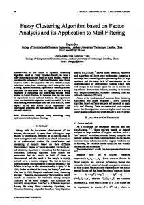
In this section some examples are presented to show the application of the proposed fuzzy similarity measure. The first example is based on a synthetic data set, and the second example deals with the visualization and clustering of the well-known wine data set. The synthetic data set contains 100 2-dimensional data objects. 99 objects are partitioned in 3 clusters with different sizes (22, 26 and 51 objects), shapes and densities, and it also contains an outlier. Figure 1(a) shows a relatively good result of the Jarvis-Patrick clustering applied on the normalized data set (k=8, l=4). The objects belonging to different clusters are marked with different markers. It can be seen that the algorithm was not able to identify the outlier object, and therefore the cluster denoted with ’+’ markers is split into 2 clusters. To show the complexity of this data set in Figure 1(b) the result of the well-known k-means clustering (k = 4) is also presented. The proposed fuzzy similarity was calculated with different k, t and α parameters. Different runs with parameters k = 3 . . . 25, t = 2 . . . 5 and α = 0.1 . . . 0.4 have been resulted in good clustering outcomes. In these cases the clusters were easily separable and the clustering rate (the number of well clustered objects/total number of objects) of 99 − 100%
was obtained. If a large value is chosen for parameter k, it is necessary to keep parameter t on a small value to avoid merging the outlier object with one of the clusters. The result of the MDS presentation based on the fuzzy distance matrix is shown in Figure 2(a). The parameter settings here were k = 7, t = 3 and α = 0.2. It can be seen that the calculated pairwise fuzzy similarity measures separate the 3 clusters and the outlier well. Figure 2(b) shows the VAT representation of the data set based on the single linkage fuzzy distances. The three clusters and the outlier are also easily separable in this figure. To find the proper similarity threshold to separate the clusters and the outlier we have drawn the single linkage dendrogram based on the fuzzy distance values of the objects (Figure 3). The dendrogram shows that the value di,j = 0.75 (di,j = 1 − si,j ) is a suitable choice to separate the clusters and the outlier from each other. Applying the single linkage agglomerative hierarchical algorithm based on the fuzzy similarities, and halting this algorithm at the threshold di,j = 0.75 results in a 100% clustering rate. This toy example illustrates that the proposed fuzzy similarity measure is able to separate the clusters with different sizes, shapes and densities, furthermore it is able to identify outliers.
1
1
0.9
0.9
0.8
0.8
0.7
0.7
0.6
0.6
0.5
0.5
0.4
0.4
0.3
0.3
0.2
0.2
0.1 0 0
0.1
0.1
0.2
0.3
0.4
0.5
0.6
0.7
0.8
0.9
(a) Jarvis-Patrick clustering
1
0 0
0.1
0.2
0.3
0.4
0.5
0.6
0.7
0.8
0.9
1
(b) k-means clustering
Fig. 1. Result of k-means and Jarvis-Patrick clustering on the normalized synthetic data set
The wine database (http://www.ics.uci.edu) consists of the chemical analysis of 178 wines from three different cultivars in the same Italian region. Each wine is characterized by 13 attributes, and there are 3 classes distinguished. Figure 4 shows the MDS projections based on the Euclidian and the fuzzy distances (k=6, t=3, α=0.2). The figures illustrate that the fuzzy distance based MDS separates the 3 clusters better. To separate the clusters we have drawn dendrograms based on the single, average and the complete linkage similarities. Using these parameters the best result (clustering rate 96.62%) is given by the average linkage based dendrogram, on which the clusters are uniquely separable.
0.4
0.3
0.2
0.1
0
−0.1
−0.2
−0.3
−0.4 −0.4
−0.3
−0.2
−0.1
0
0.1
0.2
0.3
(a) MDS based on the fuzzy distance matrix
(b) VAT based on the single linkage fuzzy distances
Fig. 2. Different graphical representations of the fuzzy distances (synthetic data set)
1 0.95 0.9 0.85 0.8 0.75 0.7 0.65 0.6 0.55 0.5
Fig. 3. Single linkage dendrogram based on the fuzzy distances (synthetic data set)
0.8
0.3
0.6
0.2 0.4
0.1 0.2
0 0
−0.1 −0.2
−0.2 −0.4
−0.3
−0.6
−0.8 −1
−0.8
−0.6
−0.4
−0.2
0
0.2
0.4
0.6
0.8
1
(a) MDS based on the Euclidian distances
−0.4 −0.4
−0.3
−0.2
−0.1
0
0.1
0.2
0.3
(b) MDS based on the fuzzy distance matrix
Fig. 4. Different MDS representations of the wine data set
4
Conclusion
In this paper we introduced a new fuzzy similarity measure that extends the similarity measure of Jarvis-Patrick algorithm in two ways: (i) it takes into account the far neighbors partway and (ii) it fuzzifies the crisp decision criterion of the JP algorithm. We demonstrated through application examples that clustering methods based on the proposed fuzzy similarity measure can discover outliers and clusters with arbitrary shapes, sizes and densities. Acknowledgement: The authors acknowledge the financial support of the Hungarian Research Found (OTKA 49534), the Bolyai Janos fellowship of the ¨ Hungarian Academy of Science and the Oveges fellowship.
References 1. K.H. Anders. A Hierarchical Graph-Clustering Approach to find Groups of Objects. Proceedings 5th ICA Workshop on Progress in Automated Map Generalization, IGN, Paris, France, 28–30 April, 2003. 2. M. Ankerst, M.M. Breunig, H-P Kriegel, and J. Sander. Optics: ordering points to identify the clustering structure. In SIGMOD 99: Proceedings of the 1999 ACM SIGMOD International Conference on Management of Data, pages 49–60, New York, NY, USA, 1999. ACM Press 3. J.C. Bezdek, and R.J. Hathaway. VAT: A Tool for Visual Assessment of (Cluster) Tendency. Proc. IJCNN 2002, IEEE Press, Piscataway, N.J., pp. 2225–2230, 2002. 4. E. Bicici, D. Yuret. Locally Scaled Density Based Clustering. In ICANNGA 2007, LNCS, 2007. 5. T.N. Doman, J.M. Cibulskis, M.J. Cibulskis, P.D. McCray, D.P. Spangler. Algorithm5: A Technique for Fuzzy Similarity Clustering of Chemical Inventories. Journal of Chemical Information and Computer Sciences 36(6): 1195–1204, 1996. 6. M. Ester, H-P Kriegel, J. Sander, and Xiaowei Xu. A density-based algorithm for discovering clusters in large spatial databases with noise. In KDD, p. 226–231, 1996. 7. S. Guha, R. Rastogi, and K. Shim. ROCK: a robust clustering algorithm for categorical attributes. In Proc. of the 15th Intl Conf. On Data Eng., p. 512–521, 1999. 8. X. Huang, W. Lai. Clustering graphs for visualization via node similarities. Journal of Visual Languages and Computing 17, pp. 225–253, 2006. 9. J.M. Huband, J.C. Bezdek, R.J. Hathaway: bigVAT: Visual assessment of cluster tendency for large data sets. Pattern Recognition 38(11): 1875–1886, 2005. 10. R.A. Jarvis, E.A. Patrick. Clustering Using a Similarity Measure Based on Shared Near Neighbors. IEEE Transactions on Computers, C22, 1025–1034, 1973. 11. G. Karypis, E-H Han, V. Kumar. Chameleon: Hierarchical Clustering Using Dynamic Modeling. IEEE Computer 32(8): 68–75, 1999. 12. C.T. Zahn. Graph-theoretical methods for detecting and describing gestalt clusters. IEEE Transaction on Computers C20:68–86, 1971. 13. A. Yao. On constructing minimum spanning trees in k-dimensional spaces and related problems. SIAM Journal on Computing, pages 721–736, 1982.