email:[jdrf;ss03v;hm1;jst]@ecs.soton.ac.uk. February 17, 2005. Abstract. In this paper we propose two distinct enhancements to the basic. âbag-of-keypointsâ ...
Improving “bag-of-keypoints” image categorisation: Generative Models and PDF-Kernels J.D.R. Farquhar
Sandor Szedmak Hongying Meng John Shawe-Taylor Image Speech and Intelligent Systems Department of Electronics and Computer Science University of Southampton Southampton, SO17 1BJ, UK email:[jdrf;ss03v;hm1;jst]@ecs.soton.ac.uk February 17, 2005 Abstract
In this paper we propose two distinct enhancements to the basic “bag-of-keypoints” image categorisation scheme proposed in [4]. In this approach images are represented as a variable sized set of local image features (keypoints). Thus, we require machine learning tools which can operate on sets of vectors. In [4] this is achieved by representing the set as a histogram over bins found by k-means. We show how this approach can be improved and generalised using Gaussian Mixture Models (GMMs). Alternatively, the set of keypoints can be represented directly as a probability density function, over which a kernel can be defined. This approach is shown to give state of the art categorisation performance. Keywords: image categorisation, “bag-of-keypoints”, GMM, SVM
1
Introduction
The performance of an image categorisation system depends mainly on two ingredients, the image representation and the classification algorithm. Ideally these two should be well matched so the classification algorithm works well with the given image representation. Traditionally, the machine vision community has focused upon developing powerful image representations for categorisation and recognition problems, such as local feature descriptors. However there is a growing realisation of the necessity to identify machine learning algorithms which can effectively exploit the information provided in these representations. Local features [14, 10] are very powerful image representation for categorisation problems, as seen by the state of the art performance of [4]. However, the image representation they produce is an unordered set of feature vectors, one for each interest point found in the image. This poses problems for most machine learning algorithms which expect a fixed dimensional feature vector 1
Image Processing
Labels
(SVM)
Classification
Classifier Learning
Classifier
Centers
(k−means)
Histograms
(SIFT)
Keypoint Identification
Histogram Generation
Test Images
Image Feature Extraction
Set of SIFT descriptors
Training Dataset
Machine Learning
Figure 1: The “bag-of-keypoints” image categorisation approach as developed in [4] as input. In [4] this problem is overcome by encoding the set of vectors as a histogram. As the set of histogram bins is fixed for all images this produces an ordered fixed length representation of the input set of feature vectors. However histogramming looses all information about the position of a keypoint within a bin – information which potentially could be useful for categorisation. In this paper we investigate alternatives to histogramming for set-of-vector type input features which may provide improved performance. In particular we investigate Gaussian Mixture Models (GMMs) as a more powerful and general alternative to histograms. We then go on to examine new kernels which have been recently proposed [7, 12] which work directly on set-of-vector inputs. The performance of these alternatives is assessed on a new benchmark generic image categorisation task and compared to state of the art approaches.
1.1
The “bag-of-keypoints” approach
In this section we describe the “bag-of-keypoints” approach to image categorisation as developed by [4]. As shown in Figure 1 this consists of three main steps; 1) image local feature extraction, 2) key-point identification and histogramming, and 3) classifier learning. We discuss each of these steps in turn. 1.1.1
Local image feature extraction
As mentioned above identification of a good image representation is key to effective image categorisation. In computer vision local descriptors have proved well-adapted to this purpose. Local descriptors are image features which are defined over a limited spatial extent. For image categorisation this locality provides robustness to partial visibility and occlusion as at least some of the descriptors should be visible in all cases. For example, at least one wheel of a car is visible from any aspect, hence a local descriptor for wheels will be robust to car viewpoint changes. For local descriptors to be useful in this way they should ideally repeatable such that the corresponding object points are detected and given (ideally) the same description when the object type undergoes the likely transformations, such as viewpoint, illumination or instance changes. Thus, in the car example we would like the wheel detector to produce the same wheel description for different types of car, imaged from different directions under different illuminations. This need has motivated the development of several scale and affine invariant image patch detectors, as well as descriptors which
2
are robust to geometric and illumination changes [10, 14]. The local descriptor generation process consists of two stages; 1) patch detection where local image patches which containing “interesting” features are identified and 2) descriptor generation where a feature vector describing the local patch is generated. In [4] a Harris affine invariant patch detector is used. This detects elliptical patches in an image which are local maxima in position of a scale adapted Harris function and a local maxima in scale of the Lapacian operator. The resulting elliptical patch is then mapped to circular region about the ellipse major axis to provide an affine invariant local image patch. Scale Invariant Feature Transform (SIFT) features [10] are then computed on this patch. SIFTs describe an image patch in terms of its Gaussian derivatives computed in 8 directions at a 4x4 grid of positions within the patch. Thus the descriptor is invariant to illumination changes in the patch and has a final size of 128 dimensions. Recently, [11] have conducted an extensive compassion of the repeatability of different local descriptors and found that SIFT descriptors generally performed best. Thus, we have used the same descriptors in this work. 1.1.2
Key-point identification and histogramming
Given a set of patch descriptions for each image the next main stage of the “bag-of-keypoints” approach is to identify a set of key-points which are in some way prototypes of a certain types of image patch. In [4] the keypoints are found using a simple k-means [15, p. 273] unsupervised learning procedure over the taring set. The key-points are then used to map each image’s set of patch descriptors to a histogram over keypoints. The identification of such key-points has two purposes; firstly it provides some robustness to descriptor variations as similar patch descriptors are mapped to the nearest key-point, and secondly as all images are mapped using the same set of key-points it provides a fixed length description of the input set of patch descriptors. Notice that this approach ignores all global geometric information about the relative positions of the image patches. As such geometric information is inherently very viewpoint dependent, removing this information provides additional robustness to viewpoint changes. However, given the subjective importance of shape in human object categorisation, it is quite surprising to this author that object categorisation systems perform as well as they do without this information. There have however been some recent efforts to re-introduce this geometric information to improve object categorisation performance [5]. As a further motivation for the key-points representation given in [4] is by analogy to the “bag-of-words” which has been very successful in text categorisation. This also looses much of the subjectively important geometric information contained in a document but provides surprisingly accurate results. The idea is that the key-points represent some form of “visual vocabulary” which allows for the description of any many types of image, perhaps including completely new categories not seen during the initial key-point identification. There is some evidence that this may indeed be true as [4] show that the keypoints computed for one categorisation task are almost as effective for a different task as ones computed specifically for that task.
3
1.1.3
Classifier Learning
The final main stage of the “bag-of-keypoints” approach is a traditional multiclass learning problem where a multi-class classifier must be learnt based upon the computed image keypoint histograms. In [4] na ive Bayes and SVM classifiers are compared for the learning task, with the SVM with a linear kernel giving significantly better performance.
2
Improving “bag-of-keypoints”
The “bag-of-keypoints” approach to image categorisation is clearly a novel and highly effect image categorisation method. However there appear to be a number of areas where its categorisation performance could be improved by application of more advanced machine learning techniques. Firstly, it is clear that the final categorisation performance depends critically on the chosen set of keypoints – they implicitly determine what differences between patch descriptors are visible to the learning algorithm for it to make categorisation decisions on. Thus, the keypoint identification should be made part of the learning process to ensure that discriminative distinctions are preserved whilst irrelevant ones are suppressed. This is analogous to the stemming techniques used in text categorisation which are designed to remove irrelevant differences whilst preserving discriminative differences. Secondly, we can view the image histogram as representing the set of input feature vectors by an estimate of their density distribution. A histogram is obviously a crude representation of this inherently continuous density profile. Thus, it would appear that by improving this density representation to more accurately represent the input feature set (with appropriate regularisation to ensure robustness to patch variations) we could improve the classifiers performance. Finally, the whole need for histogramming only arises because learning algorithms traditionally required fixed length features as input. Recently a number of kernels have been proposed [7, 12] which allow SVMs (and other kernel based learning algorithms) to work directly with sets of vectors. Allowing the learning algorithm to work directly with the input features potentially allows for superior performance as no potentially discriminative information is lost in the histogramming process. Avoiding the histogramming has the additional significant computational advantage of removing the need to perform the costly key-point identification.
3
Gaussian Mixture Models
A GMM [13] is a generative model of an input set of points where it is assumed that each point is generated independently from the same underlying probability density function (PDF). The GMM model this underlying PDF is a weighted mixture of a set of, M , Gaussian distributions each centred in a different part of the input space with its own covariance structure. That is the GMM models
4
the PDF as, P(x|p, µ, Σ) =
M X
M X
P(m)P(x|m) =
m=1
pm N (x|µm , Σm ),
(1)
m=1
where, P(m) = pm is the prior probability that a new point is generated by Gaussian m, and N (x|µm , Σm ) is the probability that the point x was generated by a Gaussian with mean µm and covariance Σm . By treating each mixture component as a keypoint it is clear that a Gaussian Mixture Model (GMMs) is a direct generalisation of the histogram for approximating a density models. However, the GMM has a number of advantages compared to histograms for representing density models. Firstly, as each component has its own covariance structure a points similarity to the keypoint is not based solely on the Euclidean distance to the keypoint but upon some local measure of the importance of different feature components. Thus different clusters can emphasise different feature components depending on the structure they are trying to represent, essentially this allows for a type of per-keypoint feature selection. Secondly, by using the probability that a mixture component generated a point, (known as the component responsibility, P(m|x)), as a generalisation of bin membership in histogram generation we obtain a much smoother (and hopefully more noise tolerant) approximation to the input sets density model. This approach also allows a point to contribute to more than one keypoint if necessary implicitly encoding more information about the position of a point into the output generalised histograms. Of course this flexibility comes at a price, as the number of parameters which much be learnt to encode a GMM with the same number of centres is much higher than for simple histograms, O(M (d2 /2 + d)) compared to O(M d). This large number of parameters poses two problems, firstly it is easily possible that there are more parameters than data points causing the learning problem to become ill-posed, secondly with so many parameters it is relatively easy for the GMM to over-fit the training data leading to poor performance on the test set. Both of these problems can be overcome (to some extent) by regularising the GMM training process.
3.1
Regularisation – MAP-EM
Usually GMMs are trained using the Expectation Maximisation (EM) [3, p. 65] algorithm to find a maximum likelihood (ML) parameter set. This is the set of ∗ parameters, θml , which maximise the data likelihood, L(X, θ), of the data set, X. That is, Y ∗ θml = argmax L(X, θ) = argmax P(x|θ), (2) θ
θ
x∈X
where the second equality follows because we assume the data points are generated independently. However, this approach suffers from the problem that the true ML solution is one which places an infinitely narrow Gaussian over some of the data points and ignores the rest. This is clearly an undesirable situation, and arises because the ML criterion does not constrain the parameters in a sensible way. In practice
5
this is not as severe a problem as it appears as EM tends to get caught in some other more acceptable local minima first. To avoid this behaviour we need to constrain the parameters of the GMM to incorporate our prior beliefs about the true solution. Such restrictions can also be used to prevent the GMM from over-fitting the data and hence should be viewed as a form of regularisation. One way of incorporating this prior information is to simply penalise low covariance solutions within the ML framework. A more principled approach within the Bayesian framework is to express our prior beliefs as a prior distribution over the GMMs parameters, P(θ|H), where H are the hyper-parameters which determine the prior. We can use this prior along with Bayes rule to compute the posterior distribution of the GMMs posterior parameters with respect to the data, P(θ|X) = P(X|θ)P(θ)/P(X). Theoretically integrating over this posterior distribution we obtain the best possible estimate of any parameter of interest, such asR responsibility of a component in generating a data sample, P(m|X2 ) = θ P(m|X2 , θ)P(θ)dθ. However, working with distributions over parameters can be cumbersome and computationally expensive, particularly as we need to integrate over the parameter distributions to compute any final result. Conjugate priors or variational approximations, such as the variational EM algorithm [13], can be used to significantly reduce the problems of the Bayesian approach. However, in this work we use the simpler single Maximum a-posterior (MAP) ∗ estimate of the GMM parameters. This is the set of parameters, θmap , which maximise the posterior data likelihood. That is, ∗ θmap = argmax P(X, θ|H) = argmax P(X|θ)P(θ|H), θ
(3)
θ
where we have assumed the data-set X is conditionally independent of the prior parameters H, so P(X, H) = P(X)P(H). Using the appropriate conjugate prior distributions for the GMMs parameters the MAP GMM parameter estimate can be computed using a simple variation to the EM algorithm, called the MAP-EM algorithm, as shown in [13]. Briefly, the MAP-EM algorithm works by adding the prior information as a penalty parameter which penalises parameter setting which have low prior probability in the log-likelihood approximation optimised by the EM algorithm. That is in MAP-EM we optimise the data log posterior, log(P(X, θ|H)) = log(P(X|θ)P(θ|H)) = log(P(X|θ)) + log(P(θ|H),
(4)
The first part of (4) is just the data likelihood as for normal EM, the second part is the penalty imposed by the prior on the parameter values. To optimise this function we use the standard EM trick� of rewriting �P P P M log(P(X|θ)) as x∈X log(P(x|θ)) = x∈X log P(x, m|θ) by the indem=1 pendence assumption and the fact that this is a mixture of M components. We then switch to optimising the change in log likelihood with respect to a previous
6
set of parameter values θ 0 , using, log(P(x|θ))
M X
P(x, m|θ) P(m|x, θ0 ) m=1 � � M X P(x|m, θ) ≥ P(m|x, θ0 ) log P(m|x, θ0 ) m=1
= log(
=
M X
m=1
P(m|x, θ0 )
� � P(m|x, θ0 ) log(P(x|m, θ)) − log(P(m|x, θ 0 )) ,
(5) (6) (7)
where the inequality follows by application of Jensen’s inequality. With respect to the optimisation problem the second term in brackets (log(P(m|x, θ 0 ))) is unimportant as it is independent of θ and can be dropped. Thus we can find the MAP GMM parameter estimate by iteratively solving the equation, (P PM (t) ) log(P(x|m, θ)) + log(P(θ|H)) (t+1) x∈X m=1 P(m|x, θ P θ = argmax (8) M subject to θ m=1 P(m|θ) = 1
The first part of this problem is identical to that solved to find the ML solution in normal EM, the second is the penalty due to the prior. To find a solution to this problem we require a formulation for the prior which is amenable to analysis. A conjugate prior where each individual mixture components parameters are treated independently is most appropriate in for this. For the case of a −1 GMM this prior consists of a normal distribution, N (µm |νm , ηm Σm ), for each −1 component Gaussian’s mean, a Wishart distribution, W(Σm |αm , βm ) for each components covariance matrix, and a Dirichlet density D(p|γ) for the vector of the component priors pm . Combining these densities together the prior over GMM parameters has the form, P(θ|H) = P(p, µ, Σ|ν, η, α, β, γ) = D(p|γ)
M Y
N (µi |νi , ηi−1 Σi )W(Σ−1 i |αi , βi ).
i=1
(9) This equation and then be substituted into (8) and the resulting equation solved for θ(t+1) using standard techniques. The derivation is long and technical but not difficult and so omitted here, the interested reader is referred to [13]. The result of this derivation is the following set of parameter update equations, P P(m|x, θ(t) ) + γm − 1 (t+1) pm = x∈X (10) P |X| + M i=1 (γi − 1) P (t) x∈X P(m|x, θ )x + νm ηm (t+1) (11) µm = P (t) x∈X P(m|x, θ ) + ηm P (t) T T x∈XP(m|x, θ )(x−µm )(x−µm ) + ηm (µm−νm )(µm−νm ) + 2βm P (12) Σ(t+1) = m (t) x∈X P(m|x, θ ) + 2αm − d
Notice, that to compute these updates we P only require the sufficient statistics of P each mixture component, specifically only x∈X P(m|x, θ(t) ), x∈X P(m|x, θ(t) )x, P and x∈X P(m|x, θ(t) )xxT . As all these statistics can be computed incrementally during a single pass through the data-set X taking time linear in the size 7
of the data-set, and (more importantly for large data-sets) space quadratic in the dimension of the data-set per-mixture component. Thus, as the number of iterations to convergence approximately linear in the data-set size, MAP-EM tends to require O(|X|2 ) time and O(M d2 ) space. A further trick used to reduce the running time of the MAP-EM algorithm is to initialise the mixture means with centre locations found by k-means, in our experience this tends to reduce the number of iterations to convergence by about a factor of three. 3.1.1
Prior determination
To use the MAP-EM training regime we need to set the prior parameters, ν, η, α, β, γ. One advantage of using conjugate priors is that these hyperparameters can be interpreted as the sufficient statistics of an additional artificial data-set. If the additional data X 0 is generated by a Gaussian mixture with M components, then in the absence of additional information, the posterior distribution of GMM parameters is, O p ∼ D(|X1O | + 1, |X2O | + 1, . . . , |XM | + 1)
µm |Σm Σ−1 m
∼
N (µ01 , |X10 |−1 Σm ) � 0 0 | |Xm | + d |Xm
∼ W
,
2
2
(13) (14)
Σ0m
�
(15)
where, Xi0 is the subset of X 0 generated by mixture component m and µ0m , Σ0m are this subset’s sample mean and covariance respectively. Comparing this to the definition of the conjugate prior (9) we see that, νm = µ0m , αm =
0 ηm = |Xm |, 0 (|Xm |
+ d)/2,
0 γm = |Xm | + 1,
(16)
0 βm = |Xm |Σ0m /2.
(17)
Thus, given some prior component means, µ0 , covariances, Σ0m , and component 0 data weights |Xm | (which are equivalent to the components prior probability 0 pm ), we can compute the equivalent hyper-parameters. Further, the importance of the prior in determining the final MAP parameters can be varied by 0 treating the component data weights, |Xm |, as different when computing the hyper-parameters governing the mean (νm , ηm ), covariance (αm , βm ) and prior probability vector (γm ). We denote these weights as Wµ , WΣ , and Wp for the mean, covariance and component prior probabilities respectively. Varying the component data weights in this way is equivalent to regularising each of the GMMs parameters independently.
3.2
Dimensionality Reduction
Regularising the GMM training using a prior goes some way to stopping it over-fitting the training set. However, the high dimensionality of the SIFT features themselves pose some problems for GMMs. Firstly, as the dimension increases the effect of noise P on the distances between points also increase, i.e. |x − (x + δ)|2 = |δ|2 = d δd2 . Thus, in high dimensions even a small additive noise can make points which were close look further way and move far apart points close together. This effect is magnified by the exponential in the Gaussian distribution, such that even small changes in distance can result in a large change in probability. 8
To reduce this effect we pre-process the feature set to reduce its dimension prior to training the GMM. Clearly, reducing the data dimension removes information from the data set. To maximise performance we wish to ensure that only information irrelevant to final classifier performance is removed. Thus, (like keypoint selection itself) dimensionality reduction must be viewed as an additional learning stage where the most relevant directions of the input featurespace are identified and the remaining noisy directions discarded. Of the many dimensionality reduction algorithms available, such as LDA, CCA etc, we have used two of the simplest in this work. 3.2.1
Principle Components Analysis
Principle Components Analysis (PCA) [3, p. 310] is probably the simplest and most widely used dimensionality reduction technique. It works by finding the directions in input space which have the largest covariance and mapping the input to this subspace, (conversely this can be seen as discarding the directions with lowest variance). The institution behind this approach is that because the directions of high covariance contain most of the information required to reconstruct the original data-set they most also contain most of the information required to discriminate the different classes. Finding the appropriate PCA sub-space is very simple as it turns out that the largest eigenvalues and eigenvectors of the data covariance matrix, correspond to the directions of largest variance in the data-set. Thus, to compute an n dimensional PCA subspace we simply compute the data covariance matrix, find its n largest eigenvalues, {λ1 , . . . , λn }, and associated eigenvectors, Un = [u1 , . . . , un ], and then map the original data to this sub-space, Xn = XUnT . Choosing the number of reduced dimensions n amounts to an additional regularisation parameter which should be found by experimentation. However, simply looking at the graph of eigenvalues can give a good indication of the best range of n as in many cases most of the variance is obviously concentrated in the top few directions with the rest having very low variance. 3.2.2
Partial Least Squares
Whilst intuitively simple one problem with PCA is that it takes no account of the class labels when identifying sub-space directions. Thus, as shown in Figure 2 if the differences between objects in the same class (intra-class variability) are much greater than the differences between objects in different classes (interclass variability) then PCA will attempt to preserve the intra-class variability and discard the (discriminatively useful) inter-class variability. Partial Least Squares (PLS) [1] is one method of overcoming this problem by taking account of the class labels when identifying sub-space directions. Intuitively PLS is a simple extension to PCA: where PCA finds directions of maximum covariance between the input data and itself, PLS finds directions of maximum covariance between the input data and the output labels, Y . Thus, finding the PLS sub-space directions consists of simply finding the largest eigenvalue and eigenvectors of the covariance matrix X T Y . Unfortunately, this not as simple as before because the matrix X T Y is not square but d × L, where L is the number of output dimensions (or the number of categories minus one for classification problems). Hence, it does not have true eigenvalue/vectors, instead
9
D1 X
X X X O
X O
X X
X X
X X X X
D2
O O O O O O O O O O O O O O O O O O O
Figure 2: Because PCA ignores the class labels it will concentrate on preserving the large variability along the inter-class boundary (direction D2) and remove the information perpendicular to the boundary (direction D1) required for classification. X
X X X O
C1
X
X X X O
C2
X O
X X
X
X X X X X
O
X
X
X
X
X
X X X X
O O O O O O O O O O O O O O O O O O O
All−at−once clustering
O O O O O O O O O O O O O O O O O O O
X
X X X O
X O
X X
X X
X X X X
O O O O O O O O O O O O O O O O O O O
Per−category clustering
Figure 3: Per-category clustering can preserve discriminative information lost during all-at-once clustering. the singular values and associated vectors must be used instead. However, a d×L matrix only has min(d, L) singular values. To obtain more than this number of sub-space directions an additional trick of deflating [15, p. 183] the input space is needed. Deflation is the process of removing an already used feature direction from the input space so the remaining directions can be re-used to extract more orthogonal feature directions. Deflation works by noting that the projection of an input data-point x onto a direction u is given by u(uT x), thus to remove this direction from the data-set we use, X − u(uT X) = (I − uuT )X. This process of finding feature directions and deflating can be repeated to find successively lower covariance directions until all the variance in the input data-set has been extracted.
3.3
Per-category training
PLS provides a way to take account of the desired outputs to minimise the amount of discriminative information lost during dimensionality reduction. However, as shown in Figure 3, this discriminative information may still be lost if the keypoint generation algorithm ignores the class labels. There do exist modifications to the k-means and GMM training algorithms which take account of the desired labels, such as MIM [16] for GMMs or LVQ [8] for kmeans. However, in this work we have simply performed the keypoint generation independently on a per-category basis, and then combining the resulting keypoints prior to histogramming. This is not a particularly efficient method of taking account of discriminative information as much effort can be duplicated fitting keypoints to non-discriminative parts of the input space. However, as shown in Figure 3, this should preserve most of the useful discriminative information, is very simple to implement, and is surprisingly effective.
10
3.4
Experiments
The algorithms presented in this section were tested on the same 7-category XEROX data-set as used in [4]1 . This consists of 1776 images in seven classes: 142 books, 125 bikes, 150 buildings, 201 cars, 792 faces, 216 phones and 150 trees. These images are all of the objects in natural settings and thus (apart from faces) the objects are in highly variable poses with substantial amounts of background clutter. As in [4] the local patches in the image were found using the multi-scale Harris affine detector with default parameters, with SIFTs as the patch descriptors. All the results presented report the average overall classification rate (CR), CR =
# correctly classified images , total # images
(18)
as obtained by 10-fold cross-validation. The variance of the classification rates across the folds is also reported in brackets. 3.4.1
Experiment 1: k-means
For comparative purposes we first conducted using the k-means key-point generation, using the different dimensionality reduction and training methods presented above. In all cases used a multi-class classifier based upon one-vsall trained SVMs. The data was zero meaned and each feature dimension was normalised to unit variance before SVM training. All the SVMs used a linear kernel with the optimal penalty parameter C found for each problem independently (though C=.05 generally gave best results). The results of these tests are presented in Table 4. These results clearly show the advantage of preserving discriminative information during keypoint generation, with per-category training consistently outperforming all-at-once training, and PLS dimensionality reduction outperforming PCA for the same number of reduced dimensions. Indeed, it appears the feature selection method used in PLS is actually able to remove nondiscriminative noise and actually improve performance. Thus the combination of per-category training and PLS dimensionality reduction improves classification performance by over 2% compared to the orginal XEROX results. Interestingly, unlike what [4] found in their original experiments, increasing the number of keypoints when using per-category labelling does not appear to have a significant effect on classification performance 3.4.2
Experiment 2: GMMs
To test the GMMs performance the same experimental methodology was used with the GMM replacing k-means for keypoint generation, and summed responsibility replacing bin membership for histogram generation. The GMMs were all trained with MAP-EM with the training set sample mean and covariance, used as the same prior for all mixture components. This prior amounts to the very weak assumption that all the data are generated by the same Gaussian. As discussed above the prior was weighted differently when determining the components mean, covariance and weight. After some initial 1 Available
from the LAVA project web-site http://www.l-a-v-a.org .
11
Dim Red Raw PCA 40d PLS 40d PCA 20d PLS 20d
Trn Type ALL Per-Cat ALL Per-Cat ALL Per-Cat ALL Per-Cat ALL Per-Cat
Number of 500 83.7 (8.7) 85.0 (6.9) 82.6 (4.3) 84.4 (8.7) 85.1 (4.9) 85.9 (4.7) 81.5 (7.8) 83.8 (7.1) 83.3 (3.3) 84.5 (6.5)
keypoints 1000 85.1 (8.3) 84.7 (8.1) 82.6 (10.8) 83.6 (4.4) 85.3 (8.3) 85.8 (6.9) 83.1 (8.2) 83.8 (7.0) 84.2 (6.8) 85.7 (5.6)
Figure 4: Classification rates for k-means keypoint generation for different numbers of keypoints (100, 250, 500, 1000), types of dimensionality reduction (raw, PCA and PLS) for different numbers of reduced dimensions (20 and 40) and training (per-category or all-at-once). All results reported are averages across 10-folds with numbers in brackets indicating the variance across the folds. The numbers in bold face indicated the best performance for a given number of keypoints. Blanks indicate results not available at press time. experiments it the best prior weightings were found to be: 0 weight on the component prior probabilities, 0.1 weight on the means, and 10 weight on the component covariance matrices. This amounts to a strong restriction on the Gaussian’s widths, a weak requirement that they be near the data mean, and no restriction on how many Gaussian’s are required, i.e. have non-zero prior probability. For per-category training the set of GMMs were combined into one single GMM by simply combining the set of Gaussians together and dividing the mixture components prior probability by the number of categories to ensure they summed to one. The results of these experiments are presented in Table 5. The results clearly show the superiority of GMM keypoint generation over k-means, where the best classification performance increases from 85.9% for kmeans + 1000 keypoints + PLS40 + Per-Cat, to 87.5% for GMM + 250 keypoints + PCA40 + Per-Cat. They also clearly demonstrate the ability of the GMM to obtain equivalent or better performance with many fewer keypoints – this is particularly apparent as a GMM with only 14 keypoints performs as well as the best kmeans keypoint generators with 1000 keypoints! Further the variance of the GMM results is also lower than kmeans implying they provide more consistent performance. The poor performance of the GMMs with the non-dimensionally reduced input features clearly indicates the problems the GMM experiences in high dimensional spaces. However, given reducing the dimension with PLS improves performance even for kmeans this is not a severe problem. Overall, these results show that the combination of preserving discriminative information using PLS dimensionality reduction and per-category training with GMM keypoint generation and summed responsibility based histogramming gives a further 2% classification performance increase over kmeans and 4% improvement over the orginal implementation.
12
Dim Red Raw PCA 40d PLS 40d PCA 20d PLS 20d
Trn Type ALL Per-Cat ALL Per-Cat ALL Per-Cat ALL Per-Cat ALL Per-Cat
Number of keypoints 14 100 250 69.8 (12.3) 81.1 (6.9) 83.0 (6.9) 82.4 (4.1) 69.2 (14.7) 81.6 (6.2) 86.0 (4.4) 86.5 (3.3) 87.5 (3.4) 72.9 (8.8) 84.0 (5.6) 85.3 (6.5) 87.0 (4.9) 87.1 (6.0) 68.3 (17.2) 81.6 (7.6) 83.2 (1.8) 83.0 (16.0) 86.8 (7.8) 87.3 (4.8) 74.0 (4.4) 82.6 (8.8) 84.7 (4.7) 86.1 (1.7) 87.2 (5.2)
Figure 5: Classification rates for GMM keypoint generation for different numbers of keypoints (14, 100, 250), types of dimensionality reduction (raw, PCA and PLS) for different numbers of reduced dimensions (20 and 40) and training (per-category or all-at-once). All results reported are averages across 10-folds with numbers in brackets indicating the variance across the folds. The numbers in bold face indicated the best performance for a given number of keypoints. Blanks indicate results not available at press time.
4
PDF-kernels
The machine learning techniques discussed so far have all focused on improving the keypoint generation and histogramming processes to produce better fixed length histograms to allow a standard SVM with a vector kernel to kernel to compare sets of vectors and learn a classifier. However, this process is clearly inefficient as the same set of keypoints must be used for all sets of vectors. A more desirable alternative would be to use a kernel which can work directly with the input sets of vectors and avoid keypoint generation completely. There has been some recent work on defining kernels for sets of vectors, such as the Matching kernel of [17], or the Convolution Kernel [6], or Kernel Principle Angles [18]. However, we use take a slightly different approach where we first model each set of vectors by a probability density function (PDF) and then in the SVM use a kernel defined over the PDFs. If we view the keypoint and histogramming techniques developed earlier as simply a method to approximate the set of vectors PDF then this can be seen as a further enhancement of this approach. The advantage of modelling each image’s set of descriptors independently are that each image model is tailored to the specific descriptor set and hence should be more accurate. Further, we avoid the significant computational cost of keypoint generation. As shown in Figure 6 using a PDF kernel consists of two stages, firstly computing the PDF model of the input set of vectors, and then computing the kernel matrix over these PDFs. We have used two existing kernel functions for PDFs, the Kullback-Liebler divergence kernel [12], and the Bhattacharyya kernel [2].
13
Image Processing
Labels
(SVM)
Classification
Classifier Learning
Classifier
Kernel
PDFs
Kernel Computation
(SIFT)
PDF Computation
Test Images
Image Feature Extraction
Set of SIFT descriptors
Training Dataset
Machine Learning
Figure 6: The PDF-kernel image categorisation approach as developed here.
4.1
The KL Divergence kernel
A common measure of the distance between two PDFs is the Kullback-Liebler (KL) divergence or relative entropy between the distributions, defined as, � � Z ∞ P1 (x) P1 (x) dx = EP1 log . (19) P1 (x) log D(P1 ||P2 ) = P2 (x) P2 (x) −∞ Unfortunately, this measure cannot be used as a kernel, firstly because it is not symmetric and secondly because it is not a valid inner product. The first problem can be easily overcome using the symmetric KL divergence, � � � � Z ∞ Z ∞ P1 (x) P2 (x) P1 (x) log P2 (x) log KL(P1 (x), P2 (x)) = dx + dx. P2 (x) P1 (x) −∞ −∞ The second problem is harder to overcome as it is unclear how to turn the KL measure of dissimilarity into an inner product measure of similarity. Following, [12], we have used the simple trick of computing the negative exponential of the KL divergence, and treating this as a kernel, KKL (P1 (x), P2 (x)) = exp{−αKL(P1 (x), P1 (x))}. The parameter α is included for numerical stability reasons and set to 0.04 in the work presented here. Whilst this trick does transform the symmetric KL divergence from a measure of dissimilarity to similarity it is unclear whether it represents a valid kernel. For this reason, from a theoretical point of view it is not safe to use this as a kernel function. However, practically, so long as the final kernel matrix is positive definite, it may still provide good performance.
4.2
Bhattacharyya kernel
An alternative measure of the similarity between two PDFs is the Bhattacharyya affinity [2], defined as, Z ∞p Kbat (P1 (x), P2 (x)) = P1 (x)P2 (x)dx. −∞
This is clearly an inner product and hence a valid kernel function. This kernel was introduced in [9] an generalised in [7] by replacing the square root by any other positive power of the inner product terms, P1 (x)P2 (x). In this work however we have only reported results for the kernel as defined above. 14
4.3
PDF computation
Before using these kernel functions we need to compute a PDF approximation for the input set of vectors. Clearly a PDF consisting of an impulse on each data-point is of little use as the similarities computed will only be non-zero if exactly the same point occurs in each set. Thus, to be robust to noise in the input features, we would like these PDFs need to be appropriately regularised. There exist many ways of computing a regularised PDF from a set of examples, such as Parzen windows [3, p. 177] or Support vector based density estimation. However, in this work we have simply used a MAP-EM trained GMM, with priors determined from the full training set mean and covariance as before. We have also only used a single Gaussian to model each input feature set because in this case there are simple analytic solutions for the symmetric KL divergence and the Bhattacharyya kernel: −1 KL(N (x|µ1 , Σ1 ), N (x|µ2 , Σ2 )) = tr(Σ1 Σ−1 2 ) + tr(Σ2 Σ1 ) − 2d −1 T +tr((Σ−1 1 + Σ2 )(µ1 − µ)2 ) (µ1 − µ2 )) d 2
− 12
(20)
−1 −1 Σ1 4 Σ2 4
Kbat (N (x|µ1 , Σ1 ), N (x|µ2 , Σ2 )) = 0.5 [Σ+ ] ∗ � � 1 T −1 T −1 T −1 exp − [µ1 Σ1 µ1 + µ2 Σ2 µ2 − µ+ Σ+ µ+ (21) 4 −1 −1 −1 where, Σ+ = (Σ−1 and µ+ = Σ−1 1 + Σ2 ) 1 µ1 + Σ2 µ2 , and tr represents the trace of the matrix.
4.4
Experiment 3: PDF Kernels
We tested the PDF Kernels on the same data-set as used above, simply replacing the keypoint generation and histogramming by per-image PDF generation and kernel computation. The computed kernel was then used directly in the SVM, the optimal penalty was found to be about 10. For the prior weights in PDF computation we again used Wp , Wµ , WΣ = (0, 0.1, 10) as this was found to give consistently good results. As we are fitting Gaussians to the data we have also used the dimensionality reduction techniques to avoid the problems of highdimensional spaces noted above. The results of these experiments are presented in Table 7. These results clearly show the advantage of using PDF kernels over the keypoint generation technique used previously, where the best performance increases by a further 2% over GMM and a significant 8% with respect to the original approach. There is clearly a problem with this approach for high dimensional spaces where performance significantly deceases in the original input space.
5
Conclusions
In this paper we have investigated enhancements to the LAVA “bag-ofkeypoints” image categorisation techniques. It was noted that the variable length nature of the set-of-vectors image representation poses significant problems for traditional machine learning techniques. Developing fixed length approximations for the set, such as LAVA’s keypoint histograms one way round 15
Dim Red Raw PCA 40d PLS 40d PCA 20d PLS 20d
Kernel KKL 85.63 (0.93) 89.91 (1.67) – 88.32 (1.5) –
type KPP 57.1 (1.5) 89.0 (1.1) 91.7 (3.9) 90.41 (0.76) 91.3 (3.2)
Figure 7: Classification rates for PDF kernel based classification for different kernel types (KL divergence kernel and Bhattacharyya), types of dimensionality reduction (raw, PCA and PLS) for different numbers of reduced dimensions (20 and 40). All results reported are averages across 10-folds with numbers in brackets indicating the variance across the folds. The numbers in bold face indicated the best performance for a given kernel type. this problem. Developing special purpose kernels for set-of-vectors inputs is another. In this work we have investigated both. Firstly, we investigated ways of improving the fixed length keypoint histograms using per-category training and PLS as ways of preserving discriminative information in keypoint generation, and GMMs to increase the representational power of the generated keypoints. In combination these techniques were found to improve overall classification rates from ≈ 83% to ≈ 88%, reducing error rates by about a quarter. We then investigated two special purposed for set-of-vectors inputs based upon first approximating the set by a PDF and then computing a kernel between these functions. When used with PLS to reduce dimensionality and prevent over-fitting problems this was found to improve classification results further to ≈ 91% representating a reduction in classification error by of almost half from 16.4% to 8.3%.
References [1] M. Barker and W. Rayens. Partial least squares for discrimination. Journal of Chemometrics, 17:166–173, 2003. [2] A. Bhattacharyya. On a measure of the divergence between two statistical populations defined by their probability distributions. Bull. Calcutta Math Soc., 35:99–110, 1943. [3] Christopher M. Bishop. Neural Networks for Pattern Recognition. Clarendon Press, Oxford, 1995. [4] G. Csurka, C. Bray, C. Dance, and L. Fan. Visual categorization with bags of keypoints. In XRCE Research Reports, XEROX. The 8th European Conference on Computer Vision - ECCV, Prague, 2004. [5] R. Fergus, P. Perona, and A. Zisserman. Object class recognition by unsupervised scale invarient learning. In ECCV 2002, 2002. [6] D. Haussler. Convolution kernels on discrete structures. Technical report, University of California at Santa Cruz, 1999. 16
[7] T. Jebra, R. Kondor, and A. Howard. Probability product kernels. Journal of Machine Learning Research, 5:819–844, 2004. [8] T. Kohonen. Self-Orginising Maps. Springer, 1995. [9] R. Kondor and T. Jebara. A kernel between sets of vectors. Proceedings of the ICML, 2003. [10] D. G. Lowe. Distinctive image features from scale-invariant keypoints. Internation Journal of computer Vision, 60(2):91–110, 2004. [11] K. Mikolajczyk and C. Schmid. A performance evaluation of local descriptors. In IEEE Conference on Computer vision and Pattern Recognition, June 2003. [12] P. J. Moreno, P. P. Ho, and N. Vasconcelos. A kullback-leibler divergence based kernel for svm classification in multimedia applications. In Neural Information Processing Systems, 2004. [13] D. Ormoneit and V. Tresp. Averaging, maximum likelihood and bayesian estimation for improving gaussian mixture probability density estimates. IEEE Trans. on Neural Networks, 9(4), 1998. [14] C. Schmid and R. Mohr. Local greyvalue invariants from image retrieval. IEEE. Trans. on Pattern Analysis and Machine Intelligence, 19(5):530– 534, 1997. [15] J Shawe-Taylor and N. Cristianini. Kernel Methods for Pattern Analysis. Cambridge University Press, 2004. [16] K. Torkkola. On feature extraction by mutual information maximization. In Proceedings of IEEE International Conference on Acoustics, Speech, and Signal Processing, volume 1, pages 821–824, 2002. [17] C. Wallraven, B. Caputo, and A.B.A. Graf. Recognition with local features: the kernel recipe. In Proceedings of ICCV 2003, volume 2, pages 257–264, 2003. [18] L. Wolf and A. Shashua. Learning over sets using kernel principle angles. Journal of Machine Learning Research, pages 913–931, 2003.
17