IEEE TRANSACTIONS ON POWER SYSTEMS, VOL. 19, NO. 4, NOVEMBER 2004
1867
Improving Market Clearing Price Prediction by Using a Committee Machine of Neural Networks Jau-Jia Guo, Student Member, IEEE, and Peter B. Luh, Fellow, IEEE
Abstract—Predicting market clearing prices is an important but difficult task, and neural networks have been widely used. A single neural network, however, may misrepresent part of the input-output data mapping that could have been correctly represented by different networks. The use of a “committee machine” composed of multiple networks can in principle alleviate such a difficulty. A major challenge for using a committee machine is to properly combine predictions from multiple networks, since the performance of individual networks is input dependent due to mapping misrepresentation. This paper presents a new method in which weighting coefficients for combining network predictions are the probabilities that individual networks capture the true input-output relationship at that prediction instant. Testing of the New England market cleaning prices demonstrates that the new method performs better than individual networks, and better than committee machines using current ensemble-averaging methods. Index Terms—Committee machines, energy price forecasting, multiple model approach, neural networks.
I. INTRODUCTION
N
EURAL NETWORKS have been widely used in many forecasting problems, including load and market clearing price (MCP) predictions for power systems [1]–[3]. The main reason for their success is that they are capable of inferring hidden relationship (mapping) in data. Such a regression capability comes from the proved property that radial basis function (RBF) and multi-layer perceptron (MLP) networks in theory are universal approximators, and can approximate any continuous function to any degree of accuracy given a sufficient number of hidden neurons [4], [5]. However, in view of reasons such as insufficient input-output data points or too many tunable parameters, in reality a single network often misrepresents part of the nonlinear input-output relationship which could have been more appropriately represented by different neural networks. For example, RBF networks are effective in exploiting local data characteristics, while MLP networks are good at capturing global data trends [6]. Therefore, a committee machine composed of multiple neural networks can in principle alleviate the misrepresentation of input-output data relationship suffered by a single network. There are two major approaches to obtain predictions for a committee machine. The first approach selects one prediction out of multiple network predictions. For example, the input Manuscript received November 16, 2003. This work was supported in part by the National Science Foundation under Grant ECS-9726577, and by Select Energy Inc. of the Northeast Utilities System. Paper no. PWRS-00642-2003. The authors are with the Department of Electrical and Computer Engineering, University of Connecticut, Storrs, CT 06279 USA (e-mail:
[email protected]). Digital Object Identifier 10.1109/TPWRS.2004.837759
Fig. 1. Schematic of an ensemble-averaging committee machine with network predictions y^ and weighting coefficients a .
space of mixtures of experts is divided into several regions (subspaces) to which different neural networks are assigned. A gating network decides which network prediction will be selected based on input data [6]. In contrast, the second approach combines predictions of multiple networks. A well-known method is the ensemble-averaging method as depicted in Fig. 1 where predictions of neural networks are linearly combined based on a straight average or the statistics of historical prediction errors [7]–[9]. The neural networks in Fig. 1 may be of different kinds, or of the same kind but with different configurations (e.g., different numbers of neurons), or identical but trained with different initial conditions. These networks are trained, perform predictions, and then are updated in a way as if they were stand-alone. A “weight calculator” generates weighting coefficients by which individual predictions are linearly combined in a “combiner.” In view that a neural network may misrepresent certain portions of the nonlinear input-output relationship, its prediction accuracy may not be constant. This is evident from MCP prediction results by using RBF and MLP networks in [1] that one network does not always outperform the other. Consequently, combining network predictions is not straightforward. The weighting coefficients of the ensemble-averaging method can reflect the overall historical prediction performance, but do not exploit the information contained in the current input data. The use of the current input data, however, is important because it could be utilized to infer which networks would provide good predictions. It is therefore clear that the ensemble-averaging method does not make the best use of all the available information, and small weights could be assigned to good predictions and large ones to poor predictions, resulting in the poor prediction performance for a committee machine. The purpose of this paper is to present a new method that exploits the current input data and the historical data to calculate weighting coefficients in a weight calculator for a better prediction combination. Our key idea to exploit the current input data is to estimate the quality of a prediction, that is, the prediction variance that
0885-8950/04$20.00 © 2004 IEEE
1868
IEEE TRANSACTIONS ON POWER SYSTEMS, VOL. 19, NO. 4, NOVEMBER 2004
is conditioned on the current input and the historical data. Although for a standard Kalman filter with linear dynamics and Gaussian noises, predication variances are independent of input and can be pre-computed offline, neural networks are nonlinear, and prediction variances depend on the current input [9], [10]. Incorporating prediction variances can obtain better weighting coefficients than not using it. For the completeness of presentation, prediction covariance matrices that will be used for the rest of the paper are briefly derived in Section II for the cases with multiple outputs based on [10]. A forecasting problem using a committee machine as the one shown in Fig. 1 is formulated in Section III where the inadequacy of individual networks due to the misrepresentation of input-output data relationship is first illustrated. Under the Multiple Model (MM) framework [11], it is assumed that the true relationship of any input-output data point follows one of the mappings of multiple networks. Based on the above formulation, a Bayesian inference-based method to calculate weighting coefficients considering the prediction qualities of networks is presented in Section IV. In our method, a weighting coefficient is shown to be evaluated by the probability that the true input-output relationship at the next prediction instant will follow a specific network mapping. The evaluation involves the combination of mode probabilities and the prediction qualities (that is, prediction covariance matrices) of individual networks where in our method a mode probability is the probability that the true input-output relationship at the current instant follows a specific mapping, and the prediction qualities are used to assess the transition possibility that the true input-output relationship switches from one mapping to another between the current instant and the next prediction instant. In Section V, numerical testing on a simple problem and the MCP prediction using the data from New England power markets demonstrates the advantage of combining multiple networks. Furthermore, the result of the MCP prediction shows that the new method has a better prediction performance than individual networks, and committee machines using current ensemble-averaging methods.
(i.i.d.), zero-mean, normal, and with a covariance matrix Furthermore, is assumed to be a deterministic function of with additive noise
.
(2) Similarly, is assumed to be i.i.d., zero-mean, normal, and with a covariance matrix . and , the conditional Given a new noisy input can be written as distribution of a new target output (3) where the new noiseless input (1). The distribution marginal distribution
is related to by can be written in terms of the
(4) Given that a neural network can model the true input-output data relationship, in (2) is undertaken by a network output where is a set of network weights. Therefore, the first term on the right-hand side of (4) is (5) in (5) can be linearized around . Similar to The term the derivation in [10] with the replacement of scalars and vectors by vectors and matrices, respectively, and with the normal prior assumption for neural weights that encourages a smooth network mapping and is equivalent to a weight-decay regularizer, it can be shown by taking the linearized network output, the Bayes’ rule, and the integral over that
(6) where
II. PREDICTION COVARIANCE MATRIX
(7)
As mentioned in the Introduction, the quality of a prediction is measured by the associated prediction variance. For a multi-output network, the prediction quality is contained in a prediction covariance matrix. The formula for a prediction covariance matrix will be briefly derived in this section. Since the derivation for a single network output is well described in [10], the following derivation for multiple outputs is extended from it. Consider a forecasting problem with a historical input-output where is a set of data set noisy inputs and is the corresponding set and of noisy target outputs. The dimensions of are and , respectively. A noisy input is related to the associated noiseless input by
(8) (9) (10)
(1)
The first exponential function in (6) results from the new input and the second one from the historical data . The term is the sum-of-squares error function with a regularization , is obtained by term, and the most probable weight vector, minimizing . Minimizing is the very step of network training. To make the integral over the weight vector analytically tractable in (6), the first and second order Taylor expansions and , respectively. The expansions are applied to and lead to are performed around (11)
where sible,
is input noise. To make the analytical estimate posis assumed to be independent, identically distributed
(12)
GUO AND LUH: IMPROVING MCP PREDICTION BY USING A COMMITTEE MACHINE OF NEURAL NETWORKS
where
1869
TABLE I TRAINING RESULTS OF RBF AND MLP NETWORKS
(13) (14) The first-order term in (12) vanishes because the gradient of at is zero. Substituting (11) and (12) into (6) and evaluating the integral gives the conditional probability distribution function of as
(15) where the mean and covariance matrix of this distribution funcand , respectively, and is tion are (16) The above covariance matrix has three components. The first component comes from output noise, the second one is related to weight uncertainties, and the third one is due to input uncerby using tainties. Furthermore, (15) is the estimate of a neural network, and in (15) is actually the network is the prediction covariance matrix or the coprediction, and variance matrix of estimated prediction errors. If a different netand in (15) will be changed accordwork is used, ingly. III. PROBLEM ILLUSTRATION AND FORMULATION In this section, the inadequacy of individual networks due to the misrepresentation of part of input-output data relationship is first illustrated, and then the formulation of a forecasting problem using a committee machine is presented. The following example illustrates that RBF and MLP neural networks ([6] and [9]) misrepresent part of the input-output data relationship. A. Problem Illustration A nonlinear function is composed of three Gaussian functions, a constant term, and an output noise
where
An RBF network and an MLP network were trained with input and output . There were 40 input-output data points with sampled in [0, 16]. To make network learning for some segments of the relationship more difficult, no data point was generated and in [16, 19], and five data points far from the centers of were generated with uniformly distributed in [19, 21] to contain the relationship of . These 45 data points formed the training set. According to the best training results obtained, the RBF network with three clusters and the MLP network with seven
Fig. 2. Plot of function y (the solid curve), the RBF network mapping (stars), and the MLP network mapping (circles).
hidden neurons were used. As summarized in Table I, the RBF network has 0.039 of mean absolute error (MAE) and 2.26% of mean absolute percentage error (MAPE). In contrast, the MAE and MAPE of the MLP network are 0.048% and 2.73%, respectively. To further examine network learning, the mappings of these two trained networks are plotted in Fig. 2 with 16 points uniformly sampled in [0, 21]. Fig. 2 clearly shows that for the first region in [0, 16] where there are 40 sampled data points, the where RBF mapping overshoots around the segment the MLP network learns better. For the second region with in [16, 19] where no training data points reside, the mappings of both networks are not good because there are no training data points available for the MLP and RBF networks to learn this portion of the relationship. In the third region, with in [19, 21], where there are five data points, the MLP network does not , where function is capture the relationship around has an upward centered at. The MLP mapping around trend and, however, the actual function reverses the rise right . This is because the MLP network tends to capture after the relationship that the majority of data contain, and five out of 45 training data points are not sufficient to learn the relationhas a ship of . In contrast, the RBF mapping around downward trend better matching the actual function since this part of the relationship is captured by one of the clusters. Generally speaking, these two network mappings complement each and . other around
1870
IEEE TRANSACTIONS ON POWER SYSTEMS, VOL. 19, NO. 4, NOVEMBER 2004
B. Problem Formulation The inadequacy of a single network can be overcome by using multiple networks. Such a concept has been established in the MM approach [11]. For example, in tracking aircraft, a flight is modeled by a finite number of models with parameters representing selected flying modes. The MM approach assumes that the aircraft follows one of the models at any time instant, and the model results are combined based on radar signals to effectively track the aircraft. The analogy to a forecasting problem using multiple networks is as follows. The true relationship of any input-output data point is assumed to follow one of the mappings of multiple networks, and network predictions are linearly combined to form the outputs of a committee machine. With such an analogy, a forecasting problem using a committee machine that consists of neural networks can be formulated in the following way. Consider a committee machine consisting of neural networks that are trained, updated, and predict in a way as if they were stand-alone. Given a new input and the his, each of these networks genertorical input-output data set . ates an estimated distribution for a new target at time The estimated distribution is described by (15) where the mean and covariance matrix of the distribution are the network prediction and prediction covariance matrix, respectively. The output of a committee machine at time is obtained by a weighted combination of individual network predictions , that is (17)
are weighting coefficients. The objective is where to determine weighting coefficients with the consideration of the prediction qualities of individual networks, i.e., prediction covariance matrices.
According to the above, the true distribution of given and , can be suboptimally decomposed in terms of estimated PDFs by using the total probability theorem as
(18) denotes the event that at time the mapping where of network is the true input-output relationship, and is the probability that the true relationship at time will follow the mapping of network given and . The condition automatically holds. is the estimate of The term by network and has been derived as in (15) with and replaced by the prediction and the prediction , respectively. Based on (15) and covariance matrix (18), the conditional mean of that meets the minimum mean square error criterion is a linear combination of network predictions, i.e., (19) Comparing (17) and (19) shows that the output of a committee would be the conditional mean if machine is set equal to . To yield an estimate of a random variable that meets the minimum mean-square error needs to be , which results in criterion, (20) B. The Determination of Weighting Coefficients
IV. SOLUTION METHODOLOGY A. The Bayesian Framework Since the main interest is to predict a new target output at the next instant and that is a vector-valued random variable, it is typical to estimate the probability distribution function (PDF) . In Section II, the conditional of given a new input and PDF of estimated by a neural network has been derived. Given that the true relationship of any input-output data point follows one of network mappings, the true conditional PDF of is further assumed to be approximated by a linear combination of the estimated conditional PDFs of generated by networks. The latter assumption is similar to one suboptimal technique in the MM approach, the generalized pseudo-Bayesian of first order method that only considers possible modes at the latest instant to avoid the exponentially increasing number of filters required for an optimal estimate [11]. The mathematical derivation is detailed next.
To evaluate , the total probability theorem will be deused. It will be shown later that in our method pends on two types of probabilities: a mode probability that the true input-output relationship follows a specific mapping at the current instant, and a mode transition probability describing the transition possibility that the true input-output relationship switches from one mapping to another between the current instant and the next prediction instant given the prediction quality of individual networks. is deAccording to the total probability theorem, composed as
(21) is independent of the new input at time Since the event , the first term on the right-hand side of (21) is rewritten as (22)
GUO AND LUH: IMPROVING MCP PREDICTION BY USING A COMMITTEE MACHINE OF NEURAL NETWORKS
which is the “mode probability,” i.e., the probability that the true relationship currently follows the mapping of neural network , or network currently is the correct “mode.” To determine the second term on the right-hand side of (21), is summarized by network approximation is made that weights through training, which is similar to the technique used in the MM approach [11]. Given network weights and a new input , predictions and prediction covariance matrices of networks are obtained. In other words, is summarized where and by are the prediction and the prediction covariance matrix of network , respectively. The formula for has been derived as in (16). As a result
1871
is the likelihood funcwhere tion of the mapping of network , and is a normalization conto maintain stant that equals . According to (20) and (24), can be expressed as
(26) where is the output of network , and is the associated covariance matrix. The second term in the pair of braces in (26) is again a mode transition probability. Combining as (25) and (26) gives
(23) is the mode transition probability assessing the likelihood that the true input-output relationship switches from one mapping to another between two consecutive instants given the prediction qualities of individual networks, i.e., prediction covariance matrices. Substituting (22) and (23) into (21) gives
(24) Equation (24) involves pairs of a mode probability and a mode transition probability, or scenarios that portray the transitions from possible at the current at the next prediction instant. For each instant to scenario where one specific mapping at the current moment is assumed to be true with a certain probability, prediction qualities are used to evaluate the transition possibility from such a specific mapping to the mapping of network . The weight calculator combines the evaluation of these scenarios to determine a weighting coefficient. Since these scenarios are the postulations considered by the weight calculator for the purpose of calculating a weighting coefficient, they do not change the way neural networks operate. The following subsections detail the evaluation of a mode probability and a mode transition probability. The formula of a mode probability can be derived by using the Bayes’ rule while a mode transition probability is determined through solving a quadratic optimization problem. 1) Mode Probability Evaluation: To evaluate a mode probability, in (22) is rewritten by using the Bayes’ rule as
(25)
(27) 2) Mode Transition Probability Evaluation: Mode transition probabilities appear twice in the above derivation: one in (24) and the other in (27). For a particular pair of in (24) represents the mode transition probability from at to at given prediction covariance matrices of individual networks. As mentioned earlier, a network learns the input-output relationship from data. Given conditioning on that is in the mapping the postulated scenario of network , the weights of network are updated by while those of other networks are not. There are postulated goes from 1 to , meaning scenarios because index of that every network is conditioned on once. As a result, two versions of optimal weight vectors for each network at any time for the scenario that at instant are required: for the time is in the mapping of network , and is in other mappings than the mapping of scenarios that network . These two versions of weight vectors lead to two sets of predictions and prediction covariance matrices that are used depending on scenarios. The next paragraph will explain how to utilize the current network updating and prediction process to obtain two versions of optimal weight vectors, predictions and prediction covariance matrices. Fig. 3 depicts one cycle of the network updating and prediction process added with an additional step to yield that generates another set of predictions and prediction covariance matrices. For neural network 1 (NN1), is is updated by . In conobtained after directly comes from without trast, updating, reflecting the scenario that the true input-output relationship at time is not in the mapping of network 1. Therefore, two sets of predictions and covariance matrices are obtained for a network by changing versions of weight by using and vectors: by using . Thus,
1872
IEEE TRANSACTIONS ON POWER SYSTEMS, VOL. 19, NO. 4, NOVEMBER 2004
, the objective is to find a weighting vector such that the sum
(31) is a vector-valued random variable with the minimum variance. Thus, the optimization problem is Fig. 3.
One cycle of the revised network updating and prediction process.
(32)
due to conditioning on
can be re-written as
Using (31), the objective function can be re-written as
.. .
(28) As learned from Section II, the prediction covariance matrices in (28) also represent the covariance matrices of estimated prediction errors of individual networks. Thus (28) is to determine the probability that the mapping of network will be the true input-output relationship given the covariance matrices of estimated prediction errors of individual networks. Evaluating (28) is conducted through solving the following , and optimization problem. Given , the linear combination of network predictions is
.. . (33) is a covariance matrix for estimated prediction erwhere rors of all the networks. The term is determined by , and the correlation coefficients between estimated prediction errors of the networks that are given as the prior knowledge1. In the denotation and are network indices, and and are network output indices. to (32) can be obtained by using the The solution quadratic programming technique. The th component of , which is the weighting coefficient assigned to the estimated prediction error of network , is the value of (28), that is
(29) that is a Subtracting both sides of (29) by the actual random variable leads to the combined prediction error as
(34) Similarly, the solution to the transition probability in (27) can be denoted as , that is
(30) and where are network prediction errors. To minimize the variance of , the statistics of individual network prediction errors are required, which is unknown. The only available at time information is the statistics of estimated network prediction errors, and hence is used instead, implying that the estimated prediction errors are linearly combined. From the above discussion, we know that for estimated preand diction errors
(35) 3) Weighting Coefficients in a Committee Machine: Combining (24), (27), (34), and (35), a weighting in a committee machine is coefficient (36) 1Correlation coefficients can be obtained by using a finite-sample approximation [9].
GUO AND LUH: IMPROVING MCP PREDICTION BY USING A COMMITTEE MACHINE OF NEURAL NETWORKS
1873
Fig. 4. Plot of actual values and predictions of the RBF network, the MLP network, and the new method.
Fig. 5.
Prediction standard deviation plot of the RBF and MLP networks.
where (37) and (38) It can be seen from (36) that a weighting coefficient is the sum effect of transitions from all the possible network . mappings at time to the mapping of network at time Furthermore, the prediction qualities of individual networks are incorporated to determine mode transition probabilities. Equation (36), (37), and (38) recursively determine weighting coare initialized to be , where is efficients. After the number of neural networks in a committee machine, the recursive sequence starts as follows. First, the mode probabilities , are evaluated. Then the weighting coefficients at at are determined by combining with the . mode transition probabilities, V. NUMERICAL RESULT AND INSIGHTS Two examples are presented in this section to show the advantage of a committee machine over individual networks. The first
example is the follow-up to Example 1 to demonstrate the usefulness of the prediction variance information. The second example is a practical application to predict average on-peak-hour MCPs in New England power markets2 by using three committee machines that consist of RBF and MLP networks. The first one uses the new method, the second one employs a straight average, and the third one utilizes the statistics of historical prediction errors. A. Study Case 1 This example shows the utilization of the prediction variance information for combining network predictions. The training set in Example 1 serves as the prediction set fed to the trained RBF and MLP networks of Example 1 in this example. The predictions and prediction standard deviations for both networks in the are plotted in Figs. 4 and 5, respecsegment with tively, since the mappings of both networks complement each and . other around Fig. 4 shows that the predictions of the RBF and MLP networks are rather close except for the areas with in [10, 12] and [19, 21] where the accuracy of individual predictions of 2New England power markets were restructured eight months ago to follow the concept of Standard Market Design, and have been using locational marginal prices since then. However, MCPs are still used in Independent Electricity Market Operator (IMO) in Ontario.
1874
TABLE II WEIGHTING COEFFICIENTS ASSIGNED TO RBF AND MCP PREDICTIONS
both networks is varying. Along with Fig. 5, it is further shown that the standard deviations of the RBF and MLP network give helpful signals regarding the prediction qualities of both networks in these two areas, which is that better predictions have smaller standard deviations and poorer predictions have larger ones. The new method utilizes the prediction variance information and the resultant weighting coefficients are listed in Table II. The grey area in the table has the weighting coefficients for data points with in [10, 12] and [19, 21], and shows that proper weightings are assigned to network predictions. Therefore, making use of the prediction variance information benefits the prediction combination. B. Study Case 2 The prediction for daily average on-peak-hour MCPs for New England power markets was tested in this example. A daily average on-peak-hour MCP is defined by the price averaging MCPs from hour 8 to hour 23. Forecasting average on-peakhour MCPs is critical because power is often transacted in the form of 16-hour energy blocks. Available data in this testing includes MCPs, loads, surplus, temperatures, oil, and gas prices. The training period is from May 1, 2001 to April 30, 2002 and the prediction period from May 1, 2002 to October 31, 2002. According to the best prediction results obtained, the RBF network uses 23 input factors and six clusters, and the MLP network uses 55 input factors and eight hidden neurons. The list of input factors is shown in Table III, and the target output and all the input factors except Summer and Winter indices are asafter the data is norsumed to have the noise of malized. The performance of the new method is compared not only with that of individual networks, but also with that of the other two other committee machines. One committee machine was implemented with the straight-averaging method, and the other was based on [8], where the correlation matrix to deter-
IEEE TRANSACTIONS ON POWER SYSTEMS, VOL. 19, NO. 4, NOVEMBER 2004
TABLE III LIST OF INPUT FACTORS TO THE RBF AND MLP NETWORKS
mine weighting coefficients is re-calculated whenever new prediction errors become available. The prediction results are tabulated in Table IV. From the table, it can be seen that the overall MAE and MAPE of the RBF network are 5.46$/MWh and 12.53%, respectively, in contrast with 6.11$/MWh and 13.40% of the MLP network. Actually, the MLP network performs better than the RBF network for the first two months, and the RBF network outperforms the MLP network for the rest of months. For the committee machines using the new method and the straight average, they both outperform individual networks. Comparing overall MAPEs, the new method is better than the RBF and MLP networks by 1.66% and 2.53%, respectively. Comparing overall MAEs, the new method is better than the RBF and MLP networks by 0.60 and 1.25 $/MWh, respectively. Furthermore, the overall performance of the committee machine using the straight-average method is better than that of the committee machine based on the historical prediction performance, and the new method in terms of the overall MAPE is even better than the straight-averaging method and the committee machine based on the historical prediction performance by 0.73% and 1.13%, respectively. Though the new method is better than individual networks, it as shown from the table did not outperform the MLP and RBF network in June and September, respectively. From the examination of the daily prediction performance in June and September, it shows that improper weighting coefficients for combining network predictions led to the inferior performance of the new method. Improper weighting coefficients occurred in two occasions. The first occasion is that a network with a poorer prediction has a relatively smaller prediction variance than the other network. The second occasion is that when the betterperformed model is changed form one network to another, the new method did not adjust weighting coefficients fast enough to keep up with the change. Furthermore, both networks concurrently under-forecasted or over-forecasted prices when the inferior performance of the new method occurred, which makes the new method outperforming individual networks harder. To explain why the new method has a better prediction performance than individual networks, Fig. 6 shows the August predictions of the RBF network, the MLP network, and the new
GUO AND LUH: IMPROVING MCP PREDICTION BY USING A COMMITTEE MACHINE OF NEURAL NETWORKS
1875
TABLE IV MCP PREDICTION PERFORMANCE COMPARISON
Fig. 6. Prediction plot of the RBF and MLP networks, and the committee machine using the new method in August 2002.
Fig. 7. Standard deviation plot of the RBF and MLP networks in August 2002.
method. Fig. 7 is the plot of the associated standard deviations of RBF and MLP predictions. It can be seen from Fig. 6 that the actual prices in August changed drastically. During that period of time, the predictions of the RBF and MLP networks were rather distinct. Fig. 7 shows the prediction standard deviations of both networks which are interweaved. Utilizing the information of prediction variances, the new method is able to assign appropriate weighting coefficients to network predictions for most of days. One more thing is worth being noted. With the assumption that input and output
noises are i.i.d., zero-mean, and normal, the distribution of a prediction error estimated by a neural network in Section II is approximated to be normal. As shown in Fig. 8, the histograms of the RBF and MLP prediction errors are normal, which means that the assumption for input and output noises is acceptable. VI. CONCLUSION This paper applies a committee machine to a forecasting problem, and develops a new method under the Multiple Model
1876
IEEE TRANSACTIONS ON POWER SYSTEMS, VOL. 19, NO. 4, NOVEMBER 2004
[3] H. R. Kassaei, A. Keyhani, T. Woung, and M. Rahman, “A hybrid fuzzy, neural network bus load modeling and predication,” IEEE Trans. Power Syst., vol. 14, pp. 718–724, May 1999. [4] E. J. Hartman, J. D. Keeler, and J. M. Kawalski, “Layered neural networks with gaussian hidden units as universal approximators,” Neural Networks, vol. 35, no. 2, pp. 210–215, 1990. [5] K. Hornik, M. Stinchcombe, and H. White, “Universal approximation of an unknown mapping and its derivatives using multilayer feedforward networks,” Neural Networks, pp. 551–560, 1990. [6] S. Haykin, Neural Networks: A Comprehensive Foundation. Englewood Cliffs, NJ: Prentice-Hall, 1985. [7] X. Yao and Y. Liu, “Making use of population information in evoltionary artificial neural networks,” IEEE Trans. Syst., Man, Cybern. B, vol. 28, pp. 417–425, June 1998. [8] B. T. Zhang and J. G. Joung, “Time series prediction using committee machines of evolutionary neural trees,” in Proc. of the Congress on Evolutionary Computation (CEC’99), vol. 1, July 1999, pp. 281–286. [9] C. M. Bishop, Neural Networks for Pattern Recognition. New York: Oxford, 1985, pp. 385–399. [10] W. A. Wright, “Bayesian approach to neural-network modeling with input uncertainty,” IEEE Trans. Neural Networks, vol. 10, pp. 1261–1270, Nov. 1999. [11] Y. Bar-Shalom and X. Li, Estimation and Tracking: Principles, Techniques, and Software. Norwood, MA: Artech House, 1993, pp. 450–453.
Fig. 8. Histograms of the RBF and MLP prediction errors.
framework to determine weighting coefficients. The weighting coefficients assigned to networks is shown to be the probabilities that individual networks capture the true input-output relationship at that prediction instant. The prediction qualities (that is, prediction covariance matrices) of individual networks are incorporated into the evaluation of the weighting coefficients. The testing results show that the new method not only performs better than the committee machines using current ensemble-averaging methods but also outperforms individual neural networks. REFERENCES [1] J. J. Guo and P. B. Luh, “Selecting input factors for clusters of gaussian radial basis function network to improve market clearing price prediction,” IEEE Trans. Power Syst., vol. 18, pp. 665–672, May 2003. [2] A. G. Bakirtzls, V. Petridls, S. J. Klartzis, M. C. Alexladls, and A. H. Malssls, “A neural network short term load forecasting model for the Greek power system,” IEEE Trans. Power Syst., vol. 11, pp. 858–863, May 1996.
Jau-Jia Guo (S’00) received the B.S. degree in engineering science from National Cheng-Kung University, Tainan, Taiwan, R.O.C., in 1993, and the M.S. degrees in physics and in electrical and computer engineering from the University of Connecticut, Storrs, in 1997 and 2000, respectively. He is currently pursuing the Ph.D. degree in the Electrical and Computer Engineering Department, University of Connecticut.
Peter B. Luh (M’80–SM’91–F’95) received the B.S. degree in electrical engineering from National Taiwan University, Taipei, Taiwan, R.O.C., in 1973, the M.S. degree in aeronautics and astronautics engineering from Massachussetts Institute of Technology, Cambridge, in 1977, and the Ph.D. degree in applied mathematics from Harvard University, Cambridge, in 1980. Since 1980, he has been with the University of Connecticut, Storrs, where he is currently a SNET Endowed Professor of Communications and Information Technologies with the Department of Electrical and Computer Engineering, and the Director of the Booth Research Center for Computer Applications. His major research interests include schedule generation and reconfiguration for manufacturing and power systems. Dr. Luh is Editor-in-Chief of the IEEE TRANSACTIONS ON AUTOMATION SCIENCE AND ENGINEERING. He was previously the Editor-in-Chief of theIEEE TRANSACTIONS ON ROBOTICS AND AUTOMATION, and an Associate Editor of the IEEE TRANSACTIONS ON AUTOMATIC CONTROL.