Improving the Load Balance of Parallel Adaptive Mesh Refined

1

Improving the Load Balance of Parallel Adaptive Mesh Refined Simulations Justin Luitjens, Qingyu Meng, Martin Berzins, Tom Henderson UUSCI-2008-007 Scientific Computing and Imaging Institute University of Utah Salt Lake City, UT 84112 USA October 22, 2008

Abstract: In order to quickly take advantage of petascale machines, which are in the near future, we must improve the performance of current codes. In the past, general-purpose adaptive codes, such as Uintah, have been shown to scale to thousands of processors. However, in order to take advantage of petascale machines these codes will have to scale to hundreds of thousands of processors. One important aspect of parallel codes is the load balance. Load imbalance can greatly hinder performance and scalability at large numbers of processors. In this paper we describe two improvements to the existing load balancer within Uintah. The first improvement involves using timings gathered at run-time in order to predict the cost of work with a high degree of accuracy allowing the work to be more effectively load balanced. The second improvement proposes a method to distributed work according to a space-filling curve more effectively by attempting to minimize the maximum amount of work assigned to any one processor. The effect of this minimization technique has been compared to load balancers within Zoltan and has shown that significant improvements are possible.

Improving the Load Balance of Parallel Adaptive Mesh Refined Simulations Justin Luitjens, Qingyu Meng, Martin Berzins, Tom Henderson November 6, 2008 School of Computing - SCI Report Abstract In order to quickly take advantage of petascale machines, which are in the near future, we must improve the performance of current codes. In the past, general-purpose adaptive codes, such as Uintah, have been shown to scale to thousands of processors. However, in order to take advantage of petascale machines these codes will have to scale to hundreds of thousands of processors. One important aspect of parallel codes is the load balance. Load imbalance can greatly hinder performance and scalability at large numbers of processors. In this paper we describe two improvements to the existing load balancer within Uintah. The first improvement involves using timings gathered at run-time in order to predict the cost of work with a high degree of accuracy allowing the work to be more effectively load balanced. The second improvement proposes a method to distributed work according to a space-filling curve more effectively by attempting to minimize the maximum amount of work assigned to any one processor. The effect of this minimization technique has been compared to load balancers within Zoltan and has shown that significant improvements are possible.

1

Introduction

The Center for Safety of Accidental Fires and Explosions (C-SAFE) simulates fires and explosions in order to improve safety by gaining a

1

better understanding of the underlying physical phenomena that affect explosions. The simulations are done using their large parallel multiphysics framework Uintah [14, 11, 19, 20, 18]. Uintah is a parallel and adaptive framework built upon the Common Component Architecture (CCA) that can be used to simulate a wide variety of problems on structured grids. By being both parallel and adaptive Uintah is able to solve large problems with a high degree of accuracy quickly [18]. With petascale computing in the near future it is important that frameworks such as Uintah utilize parallel processors efficiently. The changing grid in SAMR applications have made scalability challenging, the cost to change the grid often dominates the runtime causing performance to suffer [18, 26, 27]. However, promising scaling results have recently been shown in Uintah up to 12,000 processors and up to 32,000 processors in ALPS [4]. The scalability results between ALPS and Uintah cannot be directly compared due to significant differences in both the problems being simulated and the simulation methodologies used. One crucial requirement for scalability is the load balance. Load balancing is the process in which work is distributed across processors such that each processor has approximately the same amount of work and such that the required communication between processors is minimized. In parallel adaptive frameworks load balancing must occur whenever the grid changes. In many SAMR problems the grid changes rapidly, a single grid may be used a only a few times before a new one is required. The rapid changing of the grid can cause performance problems if the adaptive portions of the framework are not efficient enough. This has lead to the use of dynamic load balancers, which are a class of load balancers that emphasize the time to load balance. The need for varying load balancers in a large variety of codes has lead to the development of the load balancing packages such as Zoltan [5, 3, 2], Metis [15], and Jostle [24]. Zoltan is a collection of common load balancing algorithms that are designed to run quickly in parallel. By combining the various algorithms into a single package with a unified interface developers can quickly switch between a variety of algorithms choosing the best one to fit their needs. Uintah has designed its own load balancer based on space-filling curves (SFCs) and has also recently connected to the Zoltan package in order to compare against some of the standard algorithms. This paper will discuss methods used to dynamically load balance a wide variety of

2

simulations within Uintah and compare Uintah’s load balancer against some of the common algorithms found in Zoltan.

2

Uintah

The Uintah Computational Framework, is a set of parallel software components and libraries built upon the DOE common component architecture that facilitate the solution of partial differential equations (PDEs) on SAMR grids. Uintah is a sophisticated computational framework that can integrate multiple simulation components, analyze the dependencies and communication patterns between them, and efficiently execute the resulting multi-physics simulation. Uintah employs an abstract task-graph representation to describe computation and communication. Through this mechanism, Uintah components delegate decisions about parallelism to a framework component, which determines communication patterns and characterizes the computational workloads, needed for global resource optimization. This allows parallelism to be integrated between multiple components while maintaining overall scalability and allows the Uintah runtime to analyze the structure of the computation to automatically enable load balancing, data communication, parallel I/O, checkpointing and restarting capabilities. Using the task-graph simulation designers can develop large-scale parallel SAMR simulations with little understanding of the underlying parallelism. To do this the designers must specify their algorithm as a series of tasks. Each task specifies its computation and the data dependencies required by the computation. The task specifies the data dependencies by stating which variables the tasks requires in order to perform its computation along with the stencil width. In addition, tasks specify which variables they compute or modify. Using the dependency information the framework can create a task graph which specifies the order of the computation and communication. In addition, the framework is advanced enough to perform many communication optimizations like asynchronous communication and message coalescing. Uintah supports a variety of variable types that can be used by simulation components. Figure 1 show the variables that Uintah supports. Cell centered variables lie in the center of a cell, face centered variables lie on the X, Y, or Z face of a cell, node centered variables

3

11 00 11 00 11 00

111 000 111 000 111 000

11 00 00 11

11 00 11 00 11 00

11 00 00 11 (a) Cell Centered

111 000 000 111

11 00 00 11

111 000 000 111

11 00 00 11

(b) Face Centered (c) Node Centered

11111 00000 00000 11111 11111 00000 11111 00000 11111 00000

1111 0000 0000 1111

(d) Particle

Figure 1: The variable types in Uintah lie on the corners of a cell, and particle variables lie at the location of particles. Particles can be placed throughout the domain and are allowed to move throughout the simulation. The wide variety of supported variables has allowed Uintah to be used for a wide variety of applications [11, 13, 12] ranging from simulating fires and explosions to simulating human vocal chords. Parallelism is achieved in Uintah by decomposing the structured grid into a set of rectangular regions called patches that are distributed across processors. Tasks are executed on each patch and communication between patch boundaries is done automatically by the framework when needed. In order to optimize many different patch operations the framework Uintah restricts patch boundaries to occur at fixed locations. When specifying the SAMR parameters a user includes a minimum patch size which is used to create a lattice on the grid. The lattice is laid across the grid such that the lattice edges are divisible by the minimum patch size. Doing this allows Uintah to make many assumptions about patch layout which simplifies the SAMR framework making many SAMR operations faster. Uintah currently supports multiple simulation components with SAMR. Examples of these modules include the fluid dynamics code ICE [16], the particle method MPM [9], and a coupled method combining both ICE and MPM called MPMICE [8].

3

Dynamic Load Balancing

One key factor in parallel performance is the patch distribution. Patches must be distributed evenly such that each processor performs nearly the same amount of work. Failure to evenly balance the work leads to poor performance because processors with less work will complete

4

their work faster than processors with more work and will have to sit idle until the processors with more work finish. In addition, patches should be distributed such that communication is minimized. In many simulations communication is predominantly local, meaning that only a small area around each patch must be communicated from neighboring patches in order to perform calculations on that patch. If two neighboring patches are placed on the same processor then communication between those patches does not need to occur. Thus clustering patches together can lead to a large reduction in the required communication. In addition, for dynamic load balancing, it is important that the time to generate the patch distribution is small relative to the overall computation. Thus dynamic load balancing can be described as the minimization of three competing costs. 1. The cost of load imbalance 2. The cost communication 3. The cost to generate the load distribution The minimization of these three costs does not coincide. For example, the best way to minimize communication is to place all of the work on a single processor which would maximize the load imbalance. Thus any load balancing algorithm must try to balance the minimization of these three costs such that the overall runtime is minimized. The following will discuss the effects of these three costs on the overall runtime of the simulation. Load imbalance occurs when one or more processors are assigned more work than other processors. When the simulation is executing the processors that have more work will take more time to finish executing. As a result the processors with less work will typically have to wait at some point for the other processors to catch up. In an ideal load balance each processor has the same amount of work causing the processors to finish their tasks around the same time minimizing the amount of time that processers wait for each other. A large load imbalance can greatly affect the overall performance and scalability. Too much communication can also cause performance issues. Communication across the network is slow relative to the time for computation. Simulation time can easily be dominated by communication. However, if patches are placed on the same processor as their neighboring patches then communication between those patches is not needed.

5

By clustering the patches together the framework can greatly reduce the communication between patches significantly affecting the overall runtime. Finally the time to generate the load distribution can also greatly affect the overall runtime. In SAMR the grid can change often. Each time the grid changes the work must be reload balanced. If a slow load balancing algorithm is used and load balancing occurs often the time to load balance can dominate the overall runtime and in this case it may be preferable to use a faster load balancing algorithm that produces a poorer patch distribution. Most load balancing algorithms are either geometric or graph based. Geometric based algorithms partition work based on coordinate information and graph based algorithms partition work based on a weighted graph that represents both communication and computation.

3.1

Geometric Based Algorithms

Geometric based algorithms use coordinate information about the calculation to load balance the work. The computation can be represented as a series of nodes each with an assigned weight representing the amount of work associated with that node. The weighted nodes have coordinate information provided by the simulation. The domain is then partitioned into approximately equal weighted partitions explicitly minimizing goal 1. Goal 2 is not explicitly addressed with these algorithms. Instead it is implicitly addressed through the use of coordinate information. In most calculations communication is predominantly local. That is in order to make a calculation on a cell only a small region around that cell is needed. By using the coordinate data the load balancer can cluster work that is geometrically close onto the same processor reducing the communication needed. Uintah’s and Zoltan’s space-filling curve algorithms are examples of a geometric based algorithm. Other geometric based algorithms found in Zoltan include Recursive Coordinate Bisection (RCB) and Recursive Inertial Bisection (RIB) [3, 2].

3.1.1

Recursive Coordinate Bisection

Recursive Coordinate Bisection uses a bisection technique to partition the domain. The algorithm first chooses one of the coordinate axis and then splits the domain by making an appropriate perpendicular cut.

6

The position of the cut should be such that both sides of the domain have approximately equal weights. The sub-domains are then further divided by recursive application of the same splitting algorithm until the number of partitions equals the number of processors [1].

3.1.2

Recursive Inertial Bisection

Recursive Inertial Bisection was purposed to improve the load balancing result of RCB. Similar to RCB, RIB divides the domain based on the location of the objects being partitioned by use of cutting planes. But RIB introduced a more flexible method on how to choose the direction to cut the domain. The algorithm computes an eigenvector of the inertial matrix to decide the direction of the principle axis instead of a coordinate axis, so that the cutting plane will always be orthogonal to the longest direction of the domain. The domain is then recursively divided into two pieces until the number of sub domains needed is reached [25].

3.1.3

Space-Filling Curves

Other common geometric based dynamic load balancing algorithms are based on space-filling curves. Space-filling curves are fractal curves that fill the domain as they are refined. Load balancers based on these curves use the curves to cluster patches together. This is done by ordering the patches in the order that the space-filling curve traverses them. The patches are then split into approximately equal sized curve segments satisfying goal 1. Some space-filling curves move through space locally without jumping across the domain. In these cases the curve maintains locality. Meaning units of work that are close together on the curve are also close together in the domain. This implies that objects close together on the curve are more likely to communicate than objects that are further apart on the curve. Partitioning the curve clusters pathes onto the same processors as their neighbors reducing the communication. The Hilbert curve [10] is a commonly used curve for dynamic load balancing. The Hilbert curve moves through space without jumping across the domain ensuring that patches neighboring on the curve also are neighbors in space. In fact, the ordering produced by the Hilbert curve is a traversal of a subset of the communication graph. This makes the Hilbert curve ideal for load balancing algorithms. Space-filling curve based algorithms are commonly used

7

for dynamic load balancing because they are fast and result in decent partitions [6, 23, 22, 21].

3.2

Graph Based Algorithms

A parallel computation can be represented by a directional weighted graph where the nodes represent work and the edges represent communication. Each node is assigned a weight representing the cost of computation. In addition, each edge is also assigned a weight representing the cost of communication between two nodes. Graph based load balancing algorithms use this graph to partition the work by minimizing both the computation weight and the communication weight. These algorithms require a graph of the communication and computation to be explicitly formed. An example of such an algorithm is Zoltan’s Parallel HyperGraph partitioner [3, 2]. Since graph based algorithms explicitly take into account communication weights they tend to produce better load balances than geometric based algorithms. However, graph based algorithms tend to take much more time to create the load distribution than geometric based algorithms. Uintah does not explicitly form the communication graph. The cost of explicitly creating the graph along with the increased cost of load balancing associated with graph based algorithms has lead to the use of geometric based load balancers within Uintah. Because of this graph based algorithms will not be further considered in this paper.

4

Uintah’s Dynamic Load Balancing

Uintah uses a dynamic load balancer based on space-filling curves because they have been shown to quickly produce decent load balances. In order to achieve as much performance as possible Uintah has developed its own parallel space-filling curve algorithm. The load balancing algorithm can be described in the following three processes: sorting the patches by the space-filling curve, estimating the weights for the patches, and assigning the patches to processors. Each of these processes is performed on each level individually. The following will discuss those three parts and compare Uintah’s performance using both its algorithm and Zoltan’s algorithms.

8

4.1

Curve Generation

Dynamic load balancers based space-filling curves must first order patches according to the space-filling curve. Uintah does this through a highly parallel method described in [17]. This method reduces the curve generation to a parallel sorting method allowing the use of highly parallel sorting methods which have been studied in detail in the past. Each processor is given a subset of the patches to sort according to the space-filling curve. While sorting the subset of patches each processor generates a unique curve index for each of its patches that are then used to merge the curves from each processor into a single curve. Using this method the cost for generating the curve is insignificant compared to other parts of the simulation. Once the patches are sorted by the space-filling curve the curve must be partitioned into approximately equally weighted curve segments. To do this each patch must first be assigned a weight.

4.2

Weight Estimation

In order to balance the load effectively the load balancer must be able to predict the amount of work on each patch. Without an accurate prediction the load balance can suffer. For simple problems this can by modeling the computations performed on variables. For example, the ICE algorithm uses cell centered variables and performs a fixed number of calculations per each cell. Thus the cost for computing on a single patch could be represented as the following: Wp = cp + cc Nc Where cp is a constant cost per patch, cc is the constant cost per cell, and Nc is the number of cells in the patch. In order for this model to be accurate the user would have to provide constants that were proportionally accurate adding an additional layer of complexity to the user. These constants can vary from machine to machine and would need to be modified whenever changes are made to the ICE code. The model gets significantly more complicated for MPMICE simulations. In MPMICE, calculations are performed on cells, nodes, and particles. The ICE model could be expanded for an MPMICE problem as follows: Wp = cp +

9

v X

cv Nv

Where v denotes the variable type, cv denotes the constant cost per variable of type v, Nv denotes the quantity of each variable contained in the patch, and v is the following variable types: cell, node, and particle. For this model the user would have to provide four constants which would be difficult to determine. In addition, the work per node in MPMICE is not constant. MPMICE performs an iterative solve locally on each node which can converge at different rates. In order for this model to be accurate the nodes would all need to converge at close to the same rate or the model would need to be expanded in order to account for differing convergence rates. It is clear that creating accurate cost models for a simulation as complex as MPMICE is a challenging task that is prone to inaccuracies.

4.2.1

Weight Profiling

Because of the drawbacks related to accurate cost modeling Uintah uses an alterative approach which uses forecasting methods to predict the cost of each patch based on observations made at runtime. During task execution the time to complete each task is recorded and used to update a simple forecasting model which is then used to predict the time to execute on each patch in the future. This provides a mechanism to accurately predict the cost of each patch while requiring little information from the user. Uintah currently uses simple exponential smoothing as its forecasting method. This model, described in [7], has been used in a wide variety of applications because of its accuracy and simplicity. The model is as follows: Wr,t+1 = αEr,t + (1 − α)Wr,t

(1)

Where Wr,t is the predicted weight at timestep t for region r, Er,t is the actual execution time at timestep t for region r and α is a weighting factor in the range of [0,1] which represents the rate of decay on past data. This method can also be viewed as a weighted moving average where the weight on past observations decreases exponentially. A smaller value for α causes the data to put more weight on recent observations causing the forecast to respond more quickly to changes in the actual value but also causes the forecast to become more susceptible to noise. A larger value for α will cause that data to be smoother eliminating noise but also causes the forecast to react more slowly to

10

changes in the actual value. α can be defined in terms of the size of a moving average window using the following formula:

α =

2.0 T +1

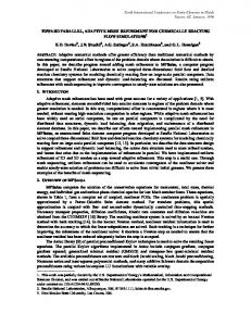
Where T is the number of timesteps that will contain 99.9% of the total weight in the weighted average [7]. Uintah uses a default value of 20 for T. On the initial timestep and when new regions are created through the AMR process Wr,t is unavailable requiring an estimation of the initial value. For this timestep Uintah uses one of the simple models specified above. While this model is likely highly inaccurate the load balance produced by it is only used for a couple of timesteps. These initial timesteps are then used to set the initial value by setting Wr,0 = Er,0 . A different initialization approach is used for new regions. The regridding process of AMR codes can produce regions that did not exist on the previous timestep. In these cases there will be no data associated with that region and an initial value must be estimated. Currently this is done by setting the initial value for new regions equal to the average cost of all regions. This ensures that the initial guess is at least close to the actual value ensuring that the estimation will be accurate within a few timesteps and that the load imbalance caused by this guess will be limited. In order to allow for changing patch sets forecasting is performed on a per region basis. The difference between regions and patches is shown in figure 2. Regions are equally size portions of the domain whose size is determined by the same lattice that is used to determine patch boundaries. Throughout the run the location and size of a region does not change. Patches are comprised of one or more regions and are allowed to change throughout the simulation. This allows for a simple mapping of costs between patches and regions. The measured cost for each region is equal to the cost of the patch times the proportion of the patch that the region encompasses as described in the following formula:

Er,t = Ep,t

11

Vr Vp

(2)

Regions

Patches

Figure 2: Regions and Patches where t is the current timestep, Er,t is the measured computation time for region r, Ep,t is the measured execution time for patch p, Vp is the volume of patch p, and Vr is the volume of region r. In addition Wp,t+1 can be defined as the sum of the weights of all regions contained in patch p:

Wp,t+1 =

r∈p X

(Wr,t+1 )

(3)

r

Uintah uses a method to store the profiling data that minimizes both storage and communication. The profile data is stored locally on each processor for each region. When a processor executes a task on a patch it adds the contribution to its local profile data using equation 2. If a region was owned by a different processor in the past then local profile data will exist on multiple processors but each processor will only update its local data. At the end of each timestep the simulation finalizes the profiling by applying formula 1. Updating the profiling data each timestep is a local operation which does not require any communication. However, communication is required when load balancing occurs. During load balancing each processor must know the cost of each patch. This is done by applying equation 3 locally and then performing an MPI Allreduce to get the global sum. In order to keep the data structures for profiling as small as possible contributions are stored in Standard Template Library (STL) maps where a region only has an entry if it is non-zero. This causes the storage per processor to be proportional to the number of patches per processor. In addition, when the contribution for a region becomes too small it is deleted from the map. When a processor has not updated a region in its map for over T timesteps then the contributing weight for that region is less than .1% of the total weight at this point we consider the weight to be insignificant and delete it from the map.

12

This prevents the size of the maps from slowly growing over time. Figure 3 shows the average absolute and relative error per patch between the predicted weight and the actual cost for an expanding 3D blastwave in ICE. The left graph shows that the primary amount of error in the predictions is caused by the finest level. This is expected as the finest level has the more work than the coarser levels and thus more potential for work. The right graph shows the mean absolute error per patch as a percentage of execution time. This graph shows that the profiling error for level 0 and level 2 are both under 10%. The error on level 1 tends to spike upward when regridding occurs. While the percentage error is higher on level 1 the amount of imbalance caused is insignificant because the overall runtime is dominated by execution on the fine level. Higher order smoothing methods described in [7] have also been used but provided no benefited over the first order smoothing described above. In the future it may be worthwhile to use advanced forecasting methods like a Kalman filter. Per Patch Mean Absolute Profiling Error

−1

Per Patch Mean Absolute Percent Profiling Error

10

25

Level 0 Level 1 Level 2

20 −2

Level 0 Level 1 Level 2

−3

Percent Error (%)

Error

10

10

15

10

−4

10

5

−5

10

10

20

30

40

50

60

70

80

90

0

100

10

timestep

20

30

40

50

60

70

80

90

100

timestep

Figure 3: The Mean Absolute and Relative Forecasting Error

4.3

Distribution Algorithm

The distribution algorithm partitions the linearly ordered patches into segments of approximately equal weight in order to minimize load imbalance. If the simulation is load balanced processors with less work will have to wait for processors with more work causing the parallel computation resource to be used inefficiently. In other words, the simulation will move at the speed of the processor with the most work. Because of this Uintah attempts to minimize both the maximum

13

amount of work assigned to any one processor and the total imbalance, where imbalance is defined as I = |1 −

Wavg | Wmax

Uintah’s curve distribution algorithm linearly traverses the patches along the curve while assigning them to processors. Two heuristics are used to determine when to partition the curve. The first heuristic attempts to minimize the imbalance by assigning the patch where it causes the least imbalance relative to the remaining work. This is done by tracking the amount of work assigned to the current processor along with the average amount of unassigned work for the remaining processors. The patch is assigned to the current processor if the imbalance caused by placing the patch on the current processor is less than the imbalance caused by not placing the patch on the current processor. The second heuristic attempts to minimize the maximum assigned work by not allowing the work on any processor to exceed some threshold. Each processor uses a different threshold in the range of (Wmax , Wavg ) where Wmax is the current maximum weight of the best known assignment and Wavg is the average amount of work per processor. This causes each processor to generate potentially different assignments and in some cases individual processors may not be able to generate a valid assignment due to the maximal constraint. Next Wmax is set to the lowest maximum found by any processor and the assignment algorithm repeats. The process is terminated when no improvements are made to Wmax . This method searches for assignment possibilities in parallel causing the algorithm to converge in few iterations. Pseudo code for this process can be found in figure 4.

5

Zoltan Results

The Uintah framework can connect to the Zoltan dynamic load balancing package. This allows the Uintah space-filling curve (USFC) code to be compared against other load balancing methods. Figure 5 shows a comparison of the total runtime for Zoltan’s load balancers normalized by Uintah’s runtime for an expanding blastwave in ICE. This graph shows that the USFC code is between 1%-11% faster than the Zoltan space-filling curve (ZHSFC) code for the full range of

14

function assignPatches(patches,weights,assignments) totalWeight=Sum(weights), averageWeight=totalWeight/numProcessors, maxWeight=totalWeight, more=true while(more) //compute local maximum weight myMaxWeight=averageWeight+(maxWeight-averageWeight)*rank/numProcessors remainingWeight=totalWeight, remainingAverageWeight=averageWeight currentWeight=0, currentProc=0 for each patch in patches takeWeight=currentWeight+weights[patch] takeImbalance=|takeWeight-remainingAverageWeight| noTakeImbalance=|currentWeight-remainingAverageWeight| if(takeImbalance