Improving the Performance of the FFT-based Parallel Code-phase ...

Presented at ION GNSS 2012, Session D3, Nashville, TN, USA, September 17-21, 2012.

Improving the Performance of the FFT-based Parallel Code-phase Search Acquisition of GNSS Signals by Decomposition of the Circular Correlation Jérôme Leclère, Cyril Botteron, Pierre-André Farine, Electronics and Signal Processing Laboratory (ESPLAB), École Polytechnique Fédérale de Lausanne (EPFL), Switzerland

Satellite System (GNSS) signals with the FFT-based Parallel Code-phase Search (PCS), and more precisely on the GPS L1 C/A signal, when the target considered is a Field Programmable Gate Array (FPGA). In this context, it is for example shown that it is possible with one of the proposed architectures to reduce the logic usage by 11 %, the memory usage by 41 %, and the Digital Signal Processing (DSP) block usage by 32 %, while keeping the same processing time. With another architecture, it is shown that the processing time can be halved by increasing the logic usage by only 35 %, while reducing the memory usage and keeping the same DSP usage. Note that the proposed approach is not based on an approximation of the traditional method, but a modified implementation providing the same result. Thus, there is no loss of sensitivity.

BIOGRAPHIES Jérôme Leclère received the Master Degree in Electronics and Signal Processing from the ENSEEIHT, Toulouse, France, in 2008. He is currently performing his Ph.D. thesis in the GNSS field at EPFL, focusing his researches in the acquisition and high sensitivity areas, with application to hardware receivers, especially using FPGAs. Dr. Cyril Botteron leads the GNSS and UWB groups in the electronics and signal processing laboratory at EPFL. He received his PhD degree from the University of Calgary, Canada, in 2003. His current research interests comprise the development of low power radio frequency (RF) integrated circuits and advanced signal processing techniques for ultra-low power communications and global and local positioning applications. Prof. Pierre-André Farine is professor in electronics and signal processing at EPFL, and is head of the electronics and signal processing laboratory. He received the M.Sc. and Ph.D. degrees in Microtechnology from the University of Neuchâtel, Switzerland, in 1978 and 1984, respectively. He is active in the study and implementation of low-power solutions for applications covering wireless telecommunications, ultra-wideband, global navigation satellite systems, and video and audio processing. He is the author or coauthor of more than 100 publications in conference and technical journals and 50 patent families (more than 270 patents).

1. INTRODUCTION The acquisition of GNSS signals consists mainly in three steps : 1) multiplication of the input signal with a local carrier replica to remove the offset in frequency due to the Doppler effect, 2) multiplication with a local pseudorandom noise (PRN) code replica; 3) Integration. The process has to be repeated for different carrier frequencies and code phases of the replicas until they are both aligned with the received ones. This is thus a two-dimension search (for each satellite). Together, the last two steps are equivalent to a circular correlation (due to the code repetition). As a consequence, the FFT can be used to compute it. This enables getting the correlation result for all the code-phases simultaneously. This is known as Parallel Code-phase Search acquisition. However, the processing time can still be relatively long, because of : 1) the different carrier frequencies to test; 2) the results over dozens or hundreds of code periods that are usually accumulated to increase the sensitivity; 3) the process has to be repeated for several satellites (up to a few dozens, if there is no a priori information and several constellations are considered). Therefore, finding new methods to perform the search faster is still topical. Within this context, we use an approach that consists in decomposing the initial circular correlation into several

ABSTRACT This paper proposes alternative architectures to perform a circular correlation using the Fast Fourier Transform (FFT) by decomposing the initial circular correlation into several smaller circular correlations. The approach used is similar to the Fast Finite Impulse Response (FIR) Algorithms (FFAs). These architectures improve the performance in terms of reduced processing time or resource usage, and consequently lower the energy consumption. The results can be applied to any system that performs circular convolution or correlation. In this paper, the application is the acquisition of Global Navigation

1

Presented at ION GNSS 2012, Session D3, Nashville, TN, USA, September 17-21, 2012. smaller circular correlations. This approach is similar to the FFAs, and the idea to combine it with the FFT to perform convolution was briefly described in [1], but the algorithms proposed were not optimal and no deep study was undertaken. Therefore, in this paper we propose and study several architectures using different numbers of FFTs that lead to different performance results. Among them, one architecture enables reducing the resources while keeping the same processing time, whereas others enable reducing the processing time, at the expense of an increase in resources. The rest of the paper is organized as follows : In Section 2, a fast review of the acquisition of GNSS signals is given. Section 3 shows how the FFT can be used to compute a circular correlation. Section 4 shows how the processing time can be reduced by duplicating elements. Section 5 presents the FFA principle and provides different architectures to reduce the processing time or the resource usage. Section 6 discusses briefly the impact on the energy consumption. In Section 7, an application example is discussed, providing details about the FPGAs and models used for the FFT and other functions. Results are first obtained using the models presented, and then checked with a real implementation of two architectures. Section 8 summarizes some important results and concludes on the impact of the proposed architectures.

this is called Parallel Frequency Search [5][6]. The search can also be parallelized in the code space, by using the FFT to get the correlation result for all the code bins simultaneously : this is the Parallel Code-phase Search (PCS) [7]. A description of these methods and their implementation on FPGAs can be found in [8]. In the following, we concentrate on the PCS, which is described in the next section.

s[n]

rf,τ[n]

∑ e j2πfn

c[n-τ] repeat for τ ∈ Τ repeat for f ∈ F

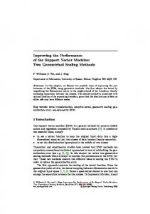
correlation Fig. 1 : Principle of the acquisition of GNSS signals 3. CIRCULAR CORRELATION USING FFT The circular correlation between two finite-length sequences x[n] and h[n] (corresponding to the input signal and code replica in our case, respectively), is defined by Eq. (1), where N is the number of samples in one period of the PRN code and * denotes the conjugate.

2. ACQUISITION OF GNSS SIGNALS Signals transmitted by GNSS satellites are a combination of a carrier, one or several PRN codes specific to each satellite, and a navigation data message [2]. When reaching the GNSS receiver, the frequency of the carrier (and of the PRN code) is different for each satellite because of the Doppler effect, and the phase of the code is unknown since the distance from the satellites is unknown assuming no a priori synchronization. After down-conversion and digitization, the GNSS receiver performs an acquisition, which consists in multiplying the signal s[n] by a carrier replica of the same frequency; then multiplying by a code replica of the same phase (and same frequency), c[n-τ], where τ is a delay; and then integrating the result over time to raise the signal out of the noise [3]. The last two steps are equivalent to a circular correlation (due to the code repetition). The corresponding schematic is shown in Fig. 1, where it can be noted that the process repeats for different phases of the code (τ belongs to T) and different carrier frequencies called bins (f belong to F). Τ and F depend on the context, such as the PRN code length, the signal modulation, the carrier frequency, the integration time or a priori information. For example, considering the GPS L1 C/A signal which PRN code is 1023-chip long (corresponding to 1 ms) and the frequency range of about ± 5 kHz (for a static user, and not including the offset of the receiver oscillator [4]), the code-phase step will be typically ½ chip resulting in 2046 code bins; and the frequency step will be typically 500 Hz for a coherent integration time of 1 ms leading to 21 frequency bins [4]. The search can be parallelized in the frequency space by looking at several or all the frequency bins using an FFT :

N 1

y[ n]   h [k ]x[(k  n) mod N ] *

(1)

k 0

In z domain formulation, the correlation becomes a product of two polynomials [9]. N

(2) Y ( z )  X ( z ) H (1 / z ) mod ( z  1) The Discrete Fourier Transform (DFT) of y[n] can be obtained by evaluating Y(z) in z = ej2πk/N, and we obtain *

*

DFT  y[n]  DFT  x[n] DFT  h[n] *

(3)

Using the FFT algorithm to implement the DFT [10], the circular correlation can thus be obtained using the Inverse FFT (IFFT), as shown by Eq. (4).

y[n]  IFFT  FFT  x[n] FFT  h[n] *

(4)

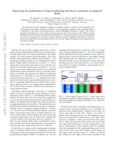
In the GNSS context, the code replica is real (for quadrature signals such as L5 and E5, the codes of pilot and data channels can be generated as complex or separately as real as well). Using this property and the fact that the conjugate of the FFT of a sequence is equal to the IFFT of the conjugate of the same sequence [11], Eq. (4) can be simplified to Eq. (5). y[n]  IFFT  FFT  x[n] IFFT  h[n] (5) The circular correlation can thus be performed using one N-point FFT, and two N-point IFFTs, as shown in Fig. 2. For the following, the architectures will be denoted as P−T−N−M, where P corresponds to ratio between the processing time of the traditional architecture provided in this section and the processing time of the architectures (neglecting the latency); T to the number of FFTs and IFFTs used; N to the transform length of the FFTs; and M

2

Presented at ION GNSS 2012, Session D3, Nashville, TN, USA, September 17-21, 2012. to the number of complex multipliers used. The traditional architecture can thus be denoted as 1−3−N−1. A simplified timing diagram is shown in Fig. 3, where the different code periods are represented by different colors. Considering that an FFT has a latency of N + L cycles, L being an intrinsic latency linked to the FFT implementation, the Kth correlation result is thus available after KN + 2N + 2L cycles.

h[n]

N

H*[k]

IFFT

N

x[n]

FFT

X[k]

Y[k]

N

IFFT

y[n]

N

Fig. 2 : Circular correlation using FFT (architecture 1−3−N−1) h[n]

h

h

h

h

x[n]

x

x

x

x

H*[k]

H*

H*

H*

H*

X[k]

X

X

X

X

Y[k]

Y

Y

Y

Y

y[n]

y L

y

y

y

L

h

h

h

xA[n]

x

x

x

xB[n]

x

x

x

*

HA [k]

*

H

H*

H*

HB*[k]

H*

H*

H*

XA[k]

X

X

X

XB[k]

X

X

X

YA[k]

Y

Y

Y

YB[k]

Y

Y

Y

yA[n]

y

y

y

yB[n]

y

y

y

y+y

y+y

y+y

xA[n]

h[n] = hA[n] + j hB[n] xB[n]

YA[k]

N

IFFT

IFFT

N

Memory 2N

IFFT

yA[n]

N

y[n]

Combination HB*[k]

H’[N-k]

XB[k]

XB[k]

N

IFFT

yB[n]

N

x

x

x

xB[n]

x

x

x

h+jh

h+jh

h+jh

H+jH

*

HA [k]

N

IFFT

H’[k]

H[k] N

H[k]

y[n] YB[k]

FFT

XA[k] HA*[k]

xA[n]

h[n]

N

XB[k]

FFT

XA[k] N

N

yA[n]

HB*[k]

FFT

Fig. 6 : Modification of the architecture 2−6−N−2 into an architecture 2−5−N−2

N

XA[k]

L

(see timing diagram in Fig. 7).

IFFT

FFT

hB[n]

4.2 Use of the real property of the PRN code replica h[n] It is known that the FFTs of two real sequences can be performed using only one FFT at the expense of a recombination afterwards [12] (details on implementation are given in Appendix B). Using this principle, we can thus use one FFT for hA[n] and hB[n], and obtain the architecture shown in Fig. 6. However, this trick increases the global latency by N cycles, and the Kth correlation result is now available after  K / 2  N  3N  2 L cycles

cycles (see timing diagram in Fig. 5), but the resources are doubled. In fact, the resources are slightly more than doubled due to the extra adder and the modified generation of the code replica. Indeed, this architecture requires the generation of two consecutive periods of the replica simultaneously (see Appendix A for more details on code replica generation). hA[n] HA*[k]

xB[n]

h

Fig. 5 : Timing diagram when the traditional architecture is duplicated (architecture 2−6−N−2)

4. REDUCTION OF THE PROCESSING TIME BY DUPLICATION 4.1 Initial Approach One of the solutions to reduce the processing time is to duplicate the architecture, as shown in Fig. 4, where the top branch can process the even periods of the code, and the bottom one the odd periods. In this case the processing time is halved (considering an even number of correlation result), since the Kth correlation result is available after  K / 2  N  2 N  2 L

hB[n]

h

L

Fig. 3 : Timing diagram of the traditional architecture (1−3−N−1)

FFT

h

y[n]

N

xA[n]

hA[n]

H+jH

H+jH

*

H*

H*

H

*

HB [k]

*

H

*

H

H*

XA[k]

X

X

X

XB[k]

X

X

X

YA[k]

Y

Y

Y

YB[k]

Y

Y

Y

yA[n]

y

y

yB[n]

y

y

y

y+y

y+y

y+y

y[n]

yB[n]

L

N

y

L

Fig. 7 : Timing diagram of the architecture 2−5−N−2

Fig. 4 : Duplication of the traditional architecture (architecture 2−6−N−2)

3

Presented at ION GNSS 2012, Session D3, Nashville, TN, USA, September 17-21, 2012. 5. FAST FIR ALGORITHMS 5.1 Introduction to FFAs Using the polyphase decomposition of filters [13], it is possible to obtain more efficient structures for FIR filters by parallelizing the processing and removing redundant computations [14][15]. A FIR filter performs a convolution, which is related to correlation; consequently we can apply the concept to the PCS. 5.2 Separation in two 5.2.1 Initial Approach We start by using the following polyphase representation (which corresponds to a separation of the signals into even and odd samples) : 1

h0[n]

N/2

h1[n]

N/2

x0[n]

1

X0[k]

FFT

N/2

x1[n]

FFT

N/2

IFFT

2

2

y1[n]

N/2

e j2πk/(N/2)

Fig. 8 : FFA-based circular correlation (architecture 2−6−N/2−5) i ∈{0;1}

N/2

1

y0[n]

IFFT

X1[k]

N/2

2

X ( z)  X 0 ( z )  z X1 ( z ) 2

H1*[k]

IFFT

Y ( z )  Y0 ( z )  z Y1 ( z ) 2

H0*[k]

IFFT

(6)

xi[n]

xi

xi

xi

xi

xi

xi

hi[n]

hi

hi

hi

hi

hi

hi

Xi[k]

Xi

Xi

Xi

Xi

Xi

Xi

Hi[k]

Hi

Hi

Hi

Hi

Hi

Hi

Yi[k]

Yi

Yi

Yi

Yi

Yi

Yi

yi

yi

yi

yi

yi

2

H ( z )  H 0 ( z )  z H1 ( z ) , where 

Yi ( z )   y[2 n  i ] z

n

n0



X i ( z )   x[2 n  i ] z

n

(7)

yi[n]

n0



H i ( z )   h[2 n  i ] z , 1

n

L

and i ∈ {0, 1}. Using Eq. (6), we can thus reformulate Eq. (2) as (the modulo operation is not shown) : 2

2

Y0 ( z )  H 0 ( z ) X 0 ( z )  H 1 ( z ) X 1 ( z ) 2

2

2

Y1 [ k ]  e

where

2

j 2  k / ( N / 2)

2

2

2

H1 [k ] X 0 [k ]  H 0 [k ] X 1 [k ] , *

5.2.2 Reduction of multipliers It is possible to reduce the number of multipliers at the expense of extra adders, as detailed in [14] and [15]. This is interesting because multipliers cost more than adders in terms of hardware. A possible solution is given in Eq. (11).

2

Y1 ( z )  z H1 ( z ) X 0 ( z )  H 0 ( z ) X 1 ( z ) Evaluating these relations in z = ej2πk/N, we obtain * * Y0 [ k ]  H 0 [ k ] X 0 [ k ]  H1 [ k ] X 1 [ k ] *

L

Fig. 9 : Timing diagram of the FFA-based architecture 2−6−N/2−5

n0

2

yi

(8)

(9)





Y0 [ k ]  H 1 [ k ]  H 0 [ k ] X 1 [k ] *

*

 H 0 [k ]  X 0 [k ]  X 1 [k ] *

Yi [ k ]  FFT  y[2n  i ] X i [ k ]  FFT  x[2 n  i ]



Y1 [ k ]  e

(10)

j 2 k / ( N / 2 )

(11)



H1 [k ]  H 0 [k ] X 0 [k ] *

*

 H 0 [k ]  X 0 [k ]  X 1 [k ] *

H i [ k ]  IFFT  h[2 n  i ] . *

The corresponding architecture is shown in Fig. 10.

and i ∈ {0, 1}. The corresponding architecture is shown in Fig. 8. The number of FFTs is doubled compared to the traditional architecture, however the transform length is halved, and there are now 5 multipliers and 2 adders. A simplified timing diagram of this architecture is shown in Fig. 9. The Kth correlation result is available after KN/2 + N + 2L cycles. Similarly as for the architectures using duplication, this architecture requires a modified generation of the code replica, since two consecutive samples of the replica must be generated simultaneously (see Appendix A).

h0[n]

IFFT

H0*[k]

N/2

h1[n]

IFFT

N/2

e j2πk/(N/2)

x0[n]

FFT

–

H1*[k]

X0[k]

–

Y0[k]

N/2

x1[n]

FFT

N/2

IFFT

y0[n]

N/2

X1[k]

Y1[k]

IFFT

y1[n]

N/2

Fig. 101 : FFA-based circular correlation with reduced number of multipliers (architecture 2−6−N/2−4) 1

4

This figure contains two typo errors : Y0[k] and Y1[k] are inverted, as well as y0[n] and y1[n].

Presented at ION GNSS 2012, Session D3, Nashville, TN, USA, September 17-21, 2012. There are now 4 multipliers, 5 adders and the generation of an exponential is required (typically using a Numerically Controlled Oscillator, or NCO). The timing diagram is not affected as compared to the architecture 2−6−N/2−5. 5.2.3 Use of the real property of the PRN code replica h[n] As described in Section 4.2, we can use only one FFT for h0[n] and h1[n], and obtain the architecture shown in Fig. 11 with the corresponding timing diagram in Fig. 12. The Kth correlation result is now available after KN/2 + 3N/2 + 2L cycles. Compared to the architecture 2−5−N−2, there are as many FFTs but the transform length is halved. We can thus expect that this architecture is more efficient, even if it has 2 extra multipliers and 4 extra adders. h[n] = h0[n] + j h1[n]

FFT

Memory

N/2

N

No reduction of multipliers

H0*[k]

H’[k]

H[k]

products with the exponential). However, for large P, the number of extra adders becomes excessive. It is then possible to use sub-optimal algorithms that still reduce the number of multipliers while keeping the increase of extra adders moderate [14][15]. Table 1 gives the complexity for the first values of P. It can be seen that for P = 2, the sub-optimal reduction gives the same result as the optimal reduction. Table 1 : Complexity of different FFAs

Combination –

e j2πk/(N/2)

x0[n]

Sub-optimal reduction of multipliers

– H1*[k]

H’[N-k]

FFT

X0[k]

Y0[k]

N/2

x1[n]

FFT

Optimal reduction of multipliers

y0[n]

IFFT

N/2

X1[k]

Y1[k]

N/2

IFFT

y1[n]

Fig. 111 : Modification of the architecture 2−6−N/2−4 into an architecture 2−5−N/2−4 i ∈{0;1}

xi[n] h[n] H[k]

xi

xi

xi

xi

xi

xi

h0 + j h1 h0 + j h1 h0 + j h1 h0 + j h1 h0 + j h1 h0 + j h1 H0 + j H1 H0 + j H1 H0 + j H1 H0 + j H1 H0 + j H1 H0 + j H1

Hi*[k]

Hi*

Hi*

Hi*

Hi*

Hi*

Hi*

Xi[k]

Xi

Xi

Xi

Xi

Xi

Xi

Yi[k]

Yi

Yi

Yi

Yi

Yi

Yi

yi

yi

yi

yi

yi

yi[n] L

yi

L

Fig. 12 : Timing diagram of the FFA-based architecture 2−5−N/2−4 5.3 Separation in P The same principle can be applied to split the signals in 3, 4, or any value. For a splitting in P (which means a reduction of the processing time by P), when the number of multipliers and FFTs is not reduced (as architecture 2−6−N/2−5), the resulting architecture is composed of - 3P (I)FFTs of N/P points - P2 + P – 1 multipliers (P² for the products between the Hi and Xj, and P – 1 for the products with the exponential) - P (P – 1) adders - 1 NCO As shown in Section 5.2.2, the number of multipliers can be reduced. The optimal reduction provides the minimum number of multipliers, which is 3P – 2 (2P – 1 for the products between the Hi and Xj [16][17], and P – 1 for the

Number of complex adders

2 3 4 2 3 4 2 3 4

5 11 19 4 8 13 4 7 10

2 6 12 5 13 25 5 25 78

H0*[k]

Memory

M0[k]

N/2

s0[n]

(I)FFT

S0[k]

N/2

s1[n]

(I)FFT

Y0[k] Combination algorithm Y1[k]

X0[k] S1[k]

X1[k]

Y[k] Memory

IFFT

y[n]

N/2

N/2

N/2

H1*[k]

Memory N/2

M1[k]

Fig. 13 : FFA-based architecture to reduce resources (architecture 1−3−N/2−M)

1

This figure contains two typo errors : Y0[k] and Y1[k] are inverted, as well as y0[n] and y1[n].

Number of complex multipliers

5.4 Application to reduce resources The FFA algorithm can also be used to reduce the resources when time multiplexing is applied. An example is shown in Fig. 13, with the corresponding timing diagram in Fig. 14. The combination algorithm to obtain Y0[k] and Y1[k] can be one of the previously presented (Eq. (9) or (11)) or an equivalent one, this is why the value of M is not specified in the caption of Fig. 13. First the inputs s0[n] and s1[n] take the value of the code replica, h0[n] and h1[n], their FFT is computed and stored in memory. During the storage, the inputs take the value of the input signal, x0[n] and x1[n]. When their FFTs are available, the memories are read, the products and combination between the Hi[k] and the Xi[k] are performed to obtain Y0[k] and Y1[k]. The IFFT of Y0[k] is computed while Y1[k] is stored in memory. Then the memory is read and the IFFT of Y1[k] is computed. This architecture requires only 3 N/2-point FFTs and two memories (Y1[k] can be stored in one of the memories used for H0*[k] and H1*[k] because the writing/reading accesses do not overlap). The throughput of this architecture is identical to the one of the traditional architecture, and the latency is slightly reduced, since the Kth correlation result is available after KN+3N/2+2L.

N/2

N/2

P

5

Presented at ION GNSS 2012, Session D3, Nashville, TN, USA, September 17-21, 2012.

si[n]

-

Digital Signal Processing (DSP) block : This is a block containing several hardware multipliers (typically 18 × 18 bits). To compare the different architectures, we will thus consider the three above elements. In addition to the resource usage of the architectures, we also consider the product resource-processing time, which corresponds to the energy consumption. Thus, to compare fairly the architectures, we define the energy efficiency as the ratio of the energy consumption of the traditional architecture over the energy consumption of the considered architecture : Eref R T (12) e  ref ref , E RT where Eref, Rref, Tref, E, R, and T are the energy consumption, the resource and the processing time of the traditional architecture and of the considered architecture, respectively. The traditional architecture has thus an energy efficiency of 1. For the other architectures, the greater is the value, the more efficient is the architecture. 7.2 Model for FFT Altera proposes several ways to implement an FFT [18]. Considering only the streaming implementation and not the buffered ones (because the computation speed is the core of the study), there are two options, fixed streaming, and variable streaming. Fixed streaming uses the block-floating point arithmetic, receives and outputs the data in natural order only, and can implement a complex multiplication using 4 real multipliers and 2 real adders (conventional representation), or using 3 real multipliers and 5 real adders (canonical representation). Variable streaming uses a fixed point arithmetic, and has the possibility to receive or output data in bit-reversed order [8][12]. This is a great advantage since it economizes memory resources and reduces the latency. However, variable streaming does not offer the choice of the implementation of complex multiplications. In Appendix C, we provide a table that summarizes the logic, memory and DSP resources consumption for Stratix III FPGAs for different transform lengths and resolutions. This is an estimation obtained from the Altera Wizard. The real resource consumption will depend on the FPGA chosen, the system implemented and the optimizations selected. However, some observations can be made. - Doubling the transform length roughly doubles the memory resources, except for some cases where the increase is lower. - For fixed streaming, doubling the transform length does not change the number of DSP elements, except between 1024 and 2048 points where the number is doubled. - For the variable streaming, in half of the cases doubling the transform length does not change the number of DSP elements, for the other half there is an increase between 16 % and 50 %. - Regarding the logic elements, doubling the transform length increase the resources by 11 % on average.

i ∈{0;1}

N/2 hi

xi

Si[k]

Hi

hi

xi

Xi

Hi

Hi*

Mi[k] Yi[k]

Yi

Y[k]

Y0

xi

Xi

Hi

Hi*

hi

xi

Xi

Hi

Hi*

Yi

y[n] L

hi

Xi Hi* Yi

Yi

Y1

Y0

Y1

Y0

Y1

Y0

Y1

y0

y1

y0

y1

y0

y1

y0

y1

L

Fig. 14 : Timing diagram of the FFA-based architecture to reduce resources (architecture 1−3−N/2−M) 6. REDUCTION OF THE ENERGY CONSUMPTION The proposed architectures also have a positive impact on the energy consumption compared to the traditional architecture. The energy consumption is the product of the processing time with the power consumption. The latter is proportional to the resources with a 1 to 1 ratio. Consequently, the reduction of the power consumption is obtained naturally for the architectures that have reduced resources. Since the processing time is unchanged, the energy consumption is also reduced. For the architectures that reduce the processing time, if the increase of resources is lower than the decrease of the processing time, the energy consumption will also be reduced. For example, if we consider an architecture that halves the processing time while the resources are increased by 50 %, its energy consumption will be 75 % of that of the initial architecture. 7. APPLICATION EXAMPLE This section presents a comparison of the different architectures when implemented on FPGAs. A low-cost FPGA family (Altera Cyclone III EP3C120) and a highend FPGA family (Altera Stratix III EP3SE260) are investigated. The GPS L1 C/A signal is considered. The main lobe of this signal is within 2.046 MHz, we consider thus a sampling frequency of 2.048 MHz, i.e. N = 2048. We first use models to determine the resource usage of the different functions in the architectures (FFT, multiplier, adder, memory). Except for the FFT, whose model is based on estimates from Altera, the models are quite straightforward and have been checked empirically. Then, a real implementation of two architectures is done to verify the accuracy of the models. 7.1 FPGA Resources An FPGA is a programmable device containing three main types of elements : - Logic block : This is a small block containing a Look-Up Table (LUT) enabling the creation of logic functions, a full adder, and one or several registers. This basis block is different for each manufacturer and even between some FPGA families - Memory block : This is a small size memory (typically between 0.5 and 128 Kibit), having multiple ports.

6

Presented at ION GNSS 2012, Session D3, Nashville, TN, USA, September 17-21, 2012. From these observations, it can be inferred that the performance of the different architectures will vary according to the initial transform length and the resolution used. To be more precise in our estimates, we have measured the resource consumption of the FFT after compilation for the cases we considered, namely 512, 1024 and 2048 points, with a resolution of 18 bits. The table is provided in Appendix C. 7.3 Model for other functions For the complex multiplications, two models are used. For Stratix III FPGAs, only the conventional representation is possible [19], a complex multiplication requires thus four real multipliers and no extra logic (the two real adders are already included in the DSP blocks). For Cyclone III FPGA, the canonical representation can be used; a complex multiplication requires thus three real multipliers and the equivalent of 8 real adders of R bits, where R is the resolution of the signals used for the complex multiplication. Regarding the complex addition, it corresponds to two real additions. And a real addition requires R logic elements (LEs, basis block of Cyclone III FPGA), or R/2 adaptive logic module (ALMs, basis block of Stratix III FPGA), where R is the resolution of the signals used for the addition. Regarding the memory, it is easy to estimate the requirements knowing the number of samples to store and their resolution. 7.4 Results from FPGA models Based on the previously described models, we have computed the estimated resource usage for different architectures (enumerated in Table 2 to Table 5). For each architecture, we have considered the different possible implementations for the FFT : - Fixed streaming, and a complex multiplier using 4 real multipliers, denoted as F4. - Fixed streaming, and a complex multiplier using 3 real multipliers, denoted as F3. - Variable streaming, and using of natural and bitreversed order, denoted V. The F3 case is considered only for Cyclone III FPGAs, since the canonical representation is not available on Stratix III. The case of variable streaming with natural order for the input and the output is not shown because the logic and memory usage is always higher than for the case of variable streaming with natural and bit-reversed order. The summary of the resource usage and energy efficiency of the architectures is provided for Stratix III FPGAs in Table 2 and Table 3, respectively, and for Cyclone FPGAs in Table 4 and Table 5, respectively. The ALM and LE columns represents the logic resources usage, the M9K column the number of 9216-bit memories used, and the last column the number of DSP 18-bit elements used (1 element corresponding to one 18-bit multiplier). The traditional architecture is the 1−3−2048−1, with an energy efficiency of 1. From Table 2 and Table 4, it can be seen that the architecture 1−3−1024−4 uses effectively

less resources than the traditional one, except for the V implementation of the FFT on Cyclone III FPGAs, which consumes 3% more of LEs. The most efficient architecture regarding the logic usage is the 4−10−512−13; the most efficient regarding the memory usage are the 4−10−512−13 and 4−10−512−10; and the most efficient regarding the DSP usage is the 2−5−1024−4. It can be noted that the architecture 2−5−1024 uses less memory than the traditional architecture for the F4 and F3 implementations of the FFT. For Stratix III FPGAs, the number of DSP elements is the same, and the logic is increased by only 40 %. For Cyclone III FPGAs, the number of DSP elements is lower considering the F4 implementation of the FFT, and equal considering the F3 implementation of the FFT, for an increase of the logic by 47 % and 35 %, respectively. Table 2 : Resource usage (model-based) of the architectures for Stratix III FPGA Number of Architecture Number of Number of DSP 18-bit (see §3) ALMs M9Ks elements P−T−N−M

F4

V

F4

V

F4

V

1−3−1024−4

10305

1−3−2048−1

11562

12042

69

51

52

64

12448

117

59

76

64

2−5−2048−2

19332

20749

213

117

128

108

2−6−1024−4

19100

22574

120

84

88

112

2−5−1024−4

16198

19079

109

79

76

96

4−12−512−13

34562

40542

240

132

196

244

4−12−512−10

35516

41496

240

132

184

232

4−10−512−13

29178

34166

209

119

172

212

4−10−512−10

30132

35120

209

119

160

200

Table 3 : Energy efficiency (model-based) of the architectures for Stratix III FPGA. The greater is the better. Architecture DSP 18-bit ALMs M9Ks (see §3) elements

7

P−T−N−M

F4

V

F4

V

F4

V

1−3−1024−4

1.12

1.03

1.70

1.16

1.46

1.00

1−3−2048−1

1

1

1

1

1

1

2−5−2048−2

1.20

1.20

1.10

1.01

1.19

1.19

2−6−1024−4

1.21

1.10

1.95

1.40

1.73

1.14

2−5−1024−4

1.43

1.30

2.15

1.49

2.00

1.33

4−12−512−13

1.34

1.23

1.95

1.79

1.55

1.05

4−12−512−10

1.30

1.20

1.95

1.79

1.65

1.10

4−10−512−13

1.59

1.46

2.24

1.98

1.77

1.21

4−10−512−10

1.53

1.42

2.24

1.98

1.90

1.28

Presented at ION GNSS 2012, Session D3, Nashville, TN, USA, September 17-21, 2012. Table 4 : Resource usage (model-based) of the architectures for Cyclone III FPGA. Number of Number of Architecture Number of LEs DSP 18-bit M9Ks elements P−T−N−M

F4

F3

V

F4 F3

V

F4 F3

V

69

86

48

39

60

1−3−2048−1

22452 27543 20535 117 117 100

75

57

63

2−5−2048−2

37591 46076 34365 213 213 185 126

96

106

2−6−1024−4

38817 43839 38837 120 120 154

84

66

108

72

57

92

1−3−1024−4

21149 23660 21159

69

2−5−1024−4

32987 37172 32992 109 109 137

4−12−512−13

72885 82701 70949 240 240 256 183 147 231

4−12−512−10

74361 84177 72425 240 240 256 174 138 222

4−10−512−13

61782 69962 60140 209 209 223 159 129 199

4−10−512−10

63258 71438 61616 209 209 223 150 120 190

Table 7 : Resource usage of the architecture 2−5−1024−4 implemented on Stratix III FPGA Number of Number of Number of Function DSP 18-bit ALMs M9Ks elements 1240 0 0 NCO 2748 20 12 FFT (h) 76 8 0 Memory 2747 20 12 FFT (x0) 2741 20 12 FFT (x1) 91 0 16 Combination 2779 20 12 IFFT (y0) 2766 20 12 IFFT (y1) 15 188 108 76 Total 8. CONCLUSIONS In this paper, we have proposed and compared several alternative architectures to perform the circular correlation using the FFT. Applying these architectures to the Parallel Code-phase Search acquisition of the GPS L1 C/A signal with an FPGA implementation, we have shown that they are more efficient than the traditional one. More specifically : the proposed architecture 1−3−1024−1 offers the same processing time as the traditional architecture (even slightly less due to reduced latency), and reduces at the same time the logic usage by 11 %, the memory by 41 % and the DSP by 32 %, considering the F4 implementation of the FFT on Stratix III FPGA; the architecture 2−5−1024−4 halves the processing time while reducing the memory resources, keeping the same DSP resources, and increasing the logic resources by only 35 %, considering the F3 implementation of the FFT on Cyclone III FPGA; and the architecture 4−10−512−13 divides the processing time by 4 while the memory resources are multiplied by only 1.79, the DSP by 2.26 and the logic by 2.52, considering the F4 implementation of the FFT on Stratix III FPGAs. This architecture also provides the best energy efficiency between the architectures compared, except for the DSP elements, where it is the 2−5−1024−4 that wins. The reason is that the 1024-point FFT uses less multipliers than the 2048-point FFT, whereas the 1024-point FFT and the 512-point FFT use the same number of multipliers (see Table 9). This shows the limit of the method, because for higher decomposition, the efficiency for DSP and logic block will stop increasing due to additional multipliers and adders required for the combination. Note that the proposed methodology can be applied to any system performing circular correlation. For future work, we will consider its application to the other GNSS signals, together with others techniques, such as the overlap-and-add method if the sampling frequency does not enable a direct use of a fast algorithm for the DFT.

Table 5 : Energy efficiency (model-based) of the architectures for Cyclone III FPGA. The greater is the better. DSP 18-bit Architecture LEs M9Ks elements P−T−N−M

F4

F3

V

1−3−1024−4

1.06

1.16

0.97

F4 F3

V

F4 F3

V

1−3−2048−1

1

1

1

2−5−2048−2

1.19

1.20

1.20

1.10 1.10 1.08 1.19 1.19 1.19

2−6−1024−4

1.16

1.26

1.06

1.95 1.95 1.30 1.79 1.73 1.17

2−5−1024−4

1.36

1.48

1.24

2.15 2.15 1.46 2.08 2.00 1.37

4−12−512−13

1.23

1.33

1.16

1.95 1.95 1.56 1.64 1.55 1.09

4−12−512−10

1.21

1.31

1.13

1.95 1.95 1.56 1.72 1.65 1.14

4−10−512−13

1.45

1.57

1.37

2.24 2.24 1.79 1.89 1.77 1.27

4−10−512−10

1.42

1.54

1.33

2.24 2.24 1.79 2.00 1.90 1.33

1.70 1.70 1.16 1.56 1.46 1.05 1

1

1

1

1

1

7.5 Results from real FPGA implementation To validate our models and conclusion, we have implemented the architectures 1−3−2048−1 and 2−5−1024−4 on a Stratix III FGPA using the F4 implementation of the FFT. Table 6 and Table 7 provide in details the resource consumption of both architectures. The energy efficiency of the architecture 2−5−1024−4 is 1.44 regarding the ALMs, 2.17 regarding the M9K, and 2.00 regarding the DSP elements. As foreseen, this architecture outperforms the traditional one, and the implementation results are very close to the estimated results. Table 6 : Resource usage of the traditional architecture implemented on Stratix III FPGA Number of Number of Number of Function DSP 18-bit ALMs M9Ks elements 3652 39 24 IFFT (h) 3596 39 24 FFT (x) 0 0 4 Multiplier 3648 39 24 IFFT (y) 10 896 117 76 Total

ACKNOWLEDGMENTS The authors would like to thank Pradyumna Ayyalasomayajula, Patrick Stadelmann and Youssef

8

Presented at ION GNSS 2012, Session D3, Nashville, TN, USA, September 17-21, 2012. Tawk for their fruitful comments that improved the quality of this paper.

[18] Altera, “FFT megacore function user guide”, 2011. [19] Altera, “Integer arithmetic megafunctions user guide”, 2012.

REFERENCES [1] M. Teixeira, M. De Jesus, and Y. Rodriguez, “Parallel FFT and parallel cyclic convolution algorithms with regular structures and no processor intercommunication,” High Performance Embedded Computing 2005, Lincoln Labs, Lexington, MA, Sept. 2005. [2] E. Kaplan, C. Hegarty, “Understanding GPS: principles and applications”, Artech House, 2005. [3] K. Borre, D. Akos, N. Bertelsen, P. Rinder, S.K. Jensen, “A software-defined GPS and Galileo receiver: a single frequency approach”, Birkhäuser Boston, 2007. [4] F. van Diggelen, “A-GPS: Assisted GPS, GNSS and SBAS”, Artech House, 2009. [5] U. Cheng, W.J. Hurd, J.I. Statman, “Spread-spectrum code acquisition in the presence of doppler shift and data modulation”, IEEE Transactions on Communications, vol. 38, no. 2, pp. 241-250, Feb. 1990. [6] H. Mathis, P. Flammant, A. Thiel, “An analytic way to optimize the detector of a post-Correlation FFT acquisition algorithm”, ION GPS/GNSS 2003, Portland, Oregon, USA, 9-12 Sept. 2003. [7] D.J.R. van Nee, A.J.R.M. Coenen, “New Fast GPS Code-Acquisition Technique using FFT”, Electronics Letters, vol. 27, no. 2, pp. 158-160, Jan. 1991. [8] J. Leclère, C. Botteron, P.-A. Farine, “Comparison framework of FPGA-based GNSS signals acquisition architectures”, IEEE Transactions on Aerospace and Electronic Systems, conditionally accepted. [9] A.V. Oppenheim, R.W. Schafer, “Discrete-time signal processing”, Prentice Hall, 2009. [10] E.O. Brigham, “The fast Fourier transform and its applications”, Prentice Hall, 1988. [11] J.O. Smith III, “Mathematics of the discrete Fourier transform (DFT), with audio applications”, W3K Publishing, 2007. [12] R.G. Lyons, “Understanding digital signal processing ”, Prentice Hall, 2010. [13] P.P. Vaidyanathan, “Multirate digital filters, filter banks, polyphase networks, and applications: a tutorial”, Proceedings of the IEEE, vol. 78, no. 1, pp. 56-93, Jan 1990. [14] Z.-J. Mou, P. Duhamel, “Short-length FIR filters and their use in fast nonrecursive filtering”, IEEE Transactions on Signal Processing, vol. 39, no. 6, pp. 1322-1332, June 1991. [15] D.A. Parker, K.K. Parhi, “Low-area/power parallel FIR digital filter implementations”, The Journal of VLSI Signal Processing, vol. 17, no. 1, pp. 75-92, Sept. 1997. [16] S. Winograd, “Arithmetic complexity of computation ”, CBMS-NSF Regional Conference Series in Applied Mathematics, SIAM Publications, 1980. [17] H.J. Nussbaumer, “Fast Fourier transform and convolution algorithms”, Springer Series in Information Sciences, 1982.

APPENDIX A : CODE REPLICA GENERATION A.1 Traditional generation An NCO is a counter with a step specifying the frequency of the output signal, as shown by Eq. (13), where M is the step, B the number of bits used for the counter, and fs the sampling frequency, at which runs the NCO [2]. f M B (13) fcode  B f s  M  code 2 2 fs At each overflow of the counter, a new chip of the PRN code is generated. The implementation of an NCO is shown in Fig. 15, and the timing diagram in Fig. 16 with fs = 2.048 MHz, fcode = 1.023 MHz, B = 32 and thus M = 2,145,386,496.

M

overflow

Adder

chip

Adder value

–1

z

z–1

Fig. 15 : Implementation of an NCO clock value

-

0

overflow

-

0

2145386496 4290772992 2141192192 4286578688 2136997888 0

0

1

0

1

∙∙∙ ∙∙∙

chip

-

0

0

0

1

1

2

∙∙∙

Fig. 16 : Timing diagram of an NCO A.2 Parallel generation of even and odd samples From Fig. 17, it can be seen that to generate simultaneously even and odd samples of the replica, we need two NCOs with different starting values and the same increment, 2M. The corresponding schematic is shown in Fig. 18, where the value at the bottom right of the adder is the value of the output at reset. clock value

-

0

M

2M

3M

4M

5M

∙∙∙

value0 value1

-

0

2M

4M

6M

8M

10M

∙∙∙

-

M

3M

5M

7M

9M

11M

∙∙∙

Fig. 17 : Timing diagram of an NCO generating even and odd samples simultaneously

2M

overflow0

Adder

0

z–1

Adder value0

0

z–1

overflow1

Adder

M

z–1

Adder value1

chip0

chip1

0

z–1

Fig. 18 : Implementation of an NCO generating even and odd samples simultaneously

9

Presented at ION GNSS 2012, Session D3, Nashville, TN, USA, September 17-21, 2012. obtained from H[k], as shown by the following equations [12].

A.3 Parallel generation of 2 consecutive periods If the number of samples per code period is an integer, such as in the previous case where there are exactly 2048 samples during one period composed of 1023 chips, the samples of the different periods will be identical, i.e. the jth samples of any period is the same as the j th sample of the first period. Consequently, two consecutive periods are identical and a classical NCO can be used. If the number of samples per code period is not an integer, the samples of the different periods will be different. Consequently, this requires a modified NCO to generate two consecutive periods. After 1 cycle, the NCO value is M mod 2B , after 2 cycles it is 2M mod 2B, and thus after k cycles it is kM mod 2B. If k=2K, this means that the value is shifted to the left K times. The modulo operation with 2B means that we keep the B least significant bits (LSBs) of the value. We can thus infer the NCO value after k cycles, by taking the B-K LSBs of the increment, and shifting it K times (or shifting the increment K times and taking the B LSBs of the result). It thus requires two NCO based on the same increment, with different starting values. Fig. 19 shows the timing diagram with fs = 2.048 MHz, fcode = 1.023001 MHz, B = 32 and thus M = 2,145,388,593 and M0 = kM mod 2B = 4294656. For the next periods, the starting value of the adder should be updated with 2M0 and 3M0, then with 4M0 and 5M0, etc., which requires each times two additions. The corresponding schematic is shown in Fig. 20.

*

H 0 [k ]  

-

0

overflowA

-

0

0

0

1

0

1

∙∙∙

chipA

-

0

0

0

1

1

2

∙∙∙

valueB

-

4294656

2149683249

104546

overflowB

-

0

0

1

0

0

1

∙∙∙

chipB

-

0

0

1

1

1

2

∙∙∙

2145388593 4290777186 2141198483 4286587076 2137008373

2145493139 4290881732 2141303029

overflow0

Adder

xM0

–1

z

Adder value0

(x+1)M0

–1

z

Adder value1

Im  H [ k ]  Im  H [ N  k ] 2

H [ N  k ]  H [k ] 2

Im  H [ k ]  Im  H [ N  k ]



(15)

2

 j

Re  H [ N  k ]  Re  H [ k ]

2 Regarding the hardware implementation, since we have to add and subtract one sequence with its N-k reverse, we need to buffer the data. The corresponding timing diagram is shown in Fig. 21. It can be seen that the writing of the samples of the second period starts while the reading of the reversed samples of the first period is not yet finished. This implies the use of two memories of N complex words, with a write access and a double read access, which will be written and read alternatively. The corresponding schematic is shown in Fig. 22. The combination block is composed of four real adders, equivalent to two complex adders, according to Eqs. (14) and (15). Note that this implementation requires an extra latency of N cycles compared to the use of two FFTs.

∙∙∙

clock

∙∙∙

H[k]

-

H[0]

H[1]

∙∙∙

w@1

-

0

1

∙∙∙

w@2

chip0

H[N-2] H[N-1]

N-2

H[0]

∙∙∙

H[1]

-

N-1

-

H[N-2] H[N-1]

0

∙∙∙

1

N-2

N-1

H[0]

H[1]

∙∙∙

0

1

∙∙∙

-

r@D

-

0

1

∙∙∙

N-2

N-1

0

1

∙∙∙

r@R

-

0

N-1

∙∙∙

2

1

0

N-1

∙∙∙

H’[k]

-

H[0]

H[1]

∙∙∙

H’[N-k]

-

H[0]

H[N-1]

∙∙∙

H0[k]

-

H0[0]

H0[1]

∙∙∙

H1[k]

-

H1[0]

H1[1]

∙∙∙

H[0]

H[1]

∙∙∙

H[0]

H[N-1]

∙∙∙

H0[N-2] H0[N-1] H0[0]

H0[1]

∙∙∙

H1[N-2] H1[N-1] H1[0]

H1[1]

∙∙∙

H[N-2] H[N-1]

H[2]

H[1]

–1

overflow1

Adder

(14)

2

H1 [k ]  j

0

z

Re  H [ N  k ]  Re  H [ k ]

*

Fig. 19 : Timing diagram of an NCO generating consecutive periods simultaneously

M

2

 j

clock valueA

H [ N  k ]  H [k ]

chip1

Fig. 21 : Timing diagram to perform two real FFTs using one complex FFT

0

z–1

Memory

Fig. 20 : Implementation of an NCO generating consecutive periods simultaneously

h0[n] + j h1[n]

APPENDIX B Let us assume that h0[n] and h1[n] are two real sequences of N points, and H0[k] and H1[k] are their corresponding DFT. We can create a new sequence h[n] = h0[n] + j h1[n], H[k] being its corresponding DFT. H0[k] and H1[k] can be

w@1 w@2

FFT

H[k] N

2N words

Memory 1 N Memory 2 N

r@D r@R H’[k]

H0[k]

Combination H’[N-k]

H1[k]

Fig. 22 : Schematic to perform two real FFTs using one complex FFT

10

Presented at ION GNSS 2012, Session D3, Nashville, TN, USA, September 17-21, 2012. APPENDIX C

Implementation

F4

V (natural to bitreversed)

V (bit-reversed to natural)

Table 8 : FFT resources on Stratix III FPGA estimated by the Altera Wizard Number of ALUTs Number of DSP 18-bit Number of M9Ks Number (Adaptive LUT, 2 ALUTs = elements 1 ALM) of points 12 bit 14 bit 16 bit 18 bit 12 bit 14 bit 16 bit 18 bit 12 bit 14 bit 16 bit 18 bit 2736 3048 3591 4265 11 11 11 11 24 24 24 24 256 2996 3368 3969 4636 11 11 11 11 24 24 24 24 512 3435 3864 4523 5248 19 19 19 19 24 24 24 24 1024 4256 4744 5692 6906 38 38 38 38 48 48 48 48 2048 4570 5093 6077 7326 57 76 76 76 48 48 48 48 4096 4400 4888 5836 7050 114 133 152 152 48 48 48 48 8192 4720 5243 6227 7477 209 247 285 304 48 48 48 48 16384 4544 5032 5980 7194 418 475 551 608 48 48 48 48 32768 4089 4483 4877 5271 1 2 2 2 16 16 20 24 256 4856 5296 5736 6176 2 3 3 3 24 24 28 32 512 5460 8930 6400 6870 4 5 6 6 24 24 28 32 1024 6211 6735 7259 7783 8 9 11 12 32 32 36 40 2048 6860 7418 7976 8534 16 18 21 23 32 32 36 40 4096 7348 7906 8464 9022 32 36 41 45 40 40 44 48 8192 7848 8406 8964 9522 63 72 81 90 40 40 44 48 16384 9297 10043 10789 11535 125 143 161 179 48 48 52 56 32768 4089 4483 4877 5271 2 2 2 2 16 16 20 24 256 4856 5296 5736 6176 3 4 4 4 24 24 28 32 512 5460 8930 6400 6870 7 7 8 8 24 24 28 32 1024 6211 6735 7259 7783 13 14 15 17 32 32 36 40 2048 6860 7418 7976 8534 27 29 31 34 32 32 36 40 4096 7348 7906 8464 9022 57 61 66 70 40 40 44 48 8192 7848 8406 8964 9522 117 126 135 144 40 40 44 48 16384 9297 10043 10789 11535 244 262 274 298 48 48 52 56 32768 Table 9 : FFT resources after compilation using a resolution of 18 bits Stratix III FPGA Cyclone III FPGA

Implementation

F4

F3 V (natural to bitreversed) V (bit-reversed to natural)

Number of points 512 1024 2048 512 1024 2048 512 1024 2048 512 1024 2048

Number of ALMs

Number of M9Ks

Number of DSP 18-bit elements

Number of LEs

Number of M9Ks

Number of DSP 18-bit elements

2735 3953 3854 3231 3546 4209 3238 3504 4030

20 20 39 11 14 19 11 14 21

12 12 24 16 16 20 16 16 20

5637 5932 7436 6455 6769 9133 5490 5947 6828 5447 5912 6735

20 20 39 20 20 39 21 26 33 22 25 34

12 12 24 9 9 18 16 16 20 16 16 20

11