INDiC: Improved Non-Intrusive load monitoring ... - Semantic Scholar

INDiC: Improved Non-Intrusive load monitoring using load Division and Calibration Nipun Batra1 , Haimonti Dutta2? , Amarjeet Singh1 1

Indraprastha Institute of Information Technology, Delhi, India {nipunb,amarjeet}@iiitd.ac.in 2 The Center for Computational Learning Systems (CCLS) Columbia University, New York, NY [email protected]

Abstract—Residential buildings contribute significantly to the overall energy consumption across most parts of the world. While smart monitoring and control of appliances can reduce the overall energy consumption, management and cost associated with such systems act as a big hindrance. Prior work has established that detailed feedback in the form of appliance level consumption to building occupants improves their awareness and paves the way for reduction in electricity consumption. Non-Intrusive Load Monitoring (NILM), i.e. the process of disaggregating the overall home electricity usage measured at the meter level into constituent appliances, provides a simple and cost effective methodology to provide such feedback to the occupants. In this paper we present Improved Non-Intrusive load monitoring using load Division and Calibration (INDiC) that simplifies NILM by dividing the appliances across multiple instrumented points (meters/phases) and calibrating the measured power. Proposed approach is used together with the Combinatorial Optimization framework and evaluated on the popular REDD dataset. Empirical evaluation, using INDiC based Combinatorial Optimization, demonstrate significant improvement in disaggregation accuracy.

I. I NTRODUCTION Buildings account for significant proportion of overall energy use in both the developing (e.g. 47% of total energy in India [1]) and the developed (e.g. 41% and 45% in US and UK respectively) countries. Modest improvements in building energy use can result in significant aggregate impact at the national scale. While several automation and management systems have been proposed for improving the operational efficiency of building systems, such systems typically lack the ability to provide detailed consumption information (e.g. appliance level consumption). Prior work [2] has shown that better feedback systems, enabling appliance level consumption, that provide insights about occupant’s energy usage information further encourages energy saving behavior resulting in 5-15% savings in electricity usage. Separately measuring each appliance’s consumption, for providing such a feedback, is both prohibitively expensive and difficult to manage. Alternatively, prior research has proposed Non Intrusive Load Monitoring (NILM) that involves disaggregating the total electricity consumption obtained at the meter level into individual appliance level consumption. Several modeling and inference approaches have been proposed (e.g. Factorial Hidden Markov Model [3] and Combinatorial Optimization [4]) in the past to address NILM with varied level of accuracy. NILM work typically assumes that all the loads are assigned to the same meter. However, many practical scenarios (e.g. commonly used split-phase supply for homes in USA and 3-phase supply for homes in India) involve load division ? The

author is also a visiting assistant professor at IIIT-Delhi.

across different phases coming at the home level. Automated assignment of different loads in a home to each phase, followed by NILM application on each phase separately, can reduce the overall modeling and inference complexity. Hereon, we follow the convention introduced in REDD [5] and generally refer to these multiple instrumented points (meters/phases) as main(s). Further, the measurements, both at the meter level and at the appliance level, are often taken with different equipment (Current Transformers, in-line measurements, ICs1 ) each with their own accuracy levels. Calibrating these diverse measurements will be beneficial for NILM modeling and inference. Grid conditions such as voltage fluctuations further motivate calibration. Motivated by these practical scenarios, we propose INDiC- Improved NILM using load Division and Calibration. Specific research contributions of our work are: •

Novel INDiC algorithm involving two simple preprocessing steps - Load division (i.e. automated assignment of different loads in a home to separate mains) and calibration (accounting for varied measurement accuracy across different equipment), that can be applied in a generic manner across several proposed NILM approaches to further improve their accuracy.

•

Extensive empirical validation, using publicly available REDD [5] dataset, establishing the effectiveness of INDiC as a preprocessing step, specifically for Combinatorial Optimization based NILM.

•

Release of open source implementation of the proposed work2 for comparative analysis with other NILM approaches as an IPython notebook [6].

We believe that this is the first extensive release of a generic NILM code base that can be used across many of the publicly available datasets and across several existing NILM modeling and inference approaches. Henceforth appliance(s) and load(s) are used interchangeably across the paper. II. R ELATED WORK Non-intrusive load monitoring was first studied by Hart [4] in the early 1990s by examining signatures in aggregated load to indicate activities of appliances. With proliferation of smart meters, the problem has gained traction in the recent times [7], [8], [9]. NILM systems can be broadly divided into two categories based on whether supervised or unsupervised disaggregation methods are used. Supervised learning techniques include optimization-based methods such as integer 1 Example

IC for power measurement is Maxim 78M6612

2 http://www.iiitd.edu.in/∼amarjeet/Research/indic.html

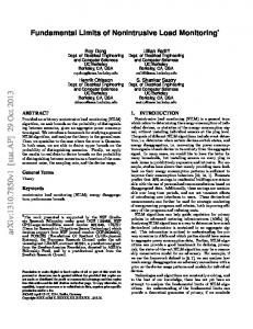
programming [10]. These approaches are compute intensive and appliances with similar or overlapping load signatures are typically difficult to discern. Other machine learning techniques (such as Artificial Neural Network (ANNs) [11] and Hidden Markov Models (HMM) [12]), have also been shown to work well for the task. Variants of HMMs such as factorial hidden Markov models (FHMMs) [3], additive FHMMs [13] and difference HMMs [14] have been studied in the context of NILM. In factorial HMMs several models evolve independently and in parallel with the observed output being a joint function of all the hidden states. Additive HMMs allow emission of a single real-valued (unobserved) output from each HMM and the output is the sum of these HMMs. In difference HMMs [14] each load is modeled using a graphical model followed by its disaggregation from the aggregate power – this process is repeated iteratively until all appliances (for which general models are available) are disaggregated. It is therefore possible to infer the probability that a change in aggregated power was generated by two consecutive states of an appliance. The applicability of these sophisticated techniques are generally hindered by the difficulty of inference from models with a large number of HMMs. Rahayu et. al. [15] proposed a discriminative model for energy disaggregation that predicts the most likely appliance state configuration from aggregated load using nonparametric classification algorithms. They posit that “subset sum” type techniques are not very effective since a large portion of the home energy is not monitored directly. In this paper, we put forward a simple idea – the aggregated load can be further split up by information on mains and knowledge about appliance assignment to mains. This would make the task of disaggregation inherently easier by solving a simpler optimization problem and most of the above sophisticated machine learning based modeling approaches can still be applied to the task3 . Several datasets have been released publicly for benchmarking energy disaggregation algorithms including REDD [5], Blued [16], AMPds [17], iAWE [18], Pecan [19] and Smart* [20]. Our empirical analysis is on the REDD data primarily because this is the most popular data set for evaluating state-of-the-art NILM approaches. III. NILM A typical NILM setup involves measuring the power mains with a smart meter and individual appliances with appliance meters for ground truth. The NILM problem in the supervised setting is formulated as predicting the power sequence for nth appliance, y n , given the measured power sequence for each appliance θn (measured using appliance meters) and the total aggregate power sequence x (measured using the smart meter). Table I summarizes the terminologies and functions used in INDiC, many of which are adopted from prior literature ([5], [14], [4]). Figure 1 shows the process of disaggregation applied to a house mains, whereby the consumption patterns of 3 appliances: refrigerator, lighting and microwave can be seen. It must be highlighted that it is improbable to instrument all the appliances in a home, thus, there will be some unaccounted 3 Combinatorial optimization is used in this work only for the purpose of illustration. There is clearly no requirement to adhere to CO alone.

(a) Aggregate home power measured by a(b) Meter power disaggregation for 3 applismart meter

ances: refrigerator, lighting and microwave, together with some unaccounted power

Fig. 1: Disaggregating a home’s electrical mains power, which can also be seen in the figure. We now explain the Combinatorial Optimization framework initially proposed by Hart [4] for solving NILM. TABLE I: Terminologies and Functions Symbol t ∈ 1, ..T n ∈ 1, ..N n θ n = {θ1n , ..., θT } M M θ M1 = {θ1 1 , ..., θT 1 } M2

θ M2 = {θ1

M

, ..., θT 2 }

Meaning Time slice Appliance number Measured power sequence for nth appliance Measured power sequence for main 1 Measured power sequence for main 2

x = {x1 , .., xT } =

Measured aggregate power sequence

θ M1 + θ M2 e = {e1 , ..., eT } p Ni where i ∈ {1, · · · , p} n y n = {y1n , ..yT }

Aggregate noise power sequence Number of electrical mains in a home Number of loads in ith main Predicted power sequence for nth appliance

k ∈ 1, ..K

Appliance power state eg. Stove has 2 states: On and Off Appliance state sequence for nth

n z n = {z1n , ..zT }

appliance,zin ∈ [1, ..K] n zt,k n

µ

Whether nth appliance is in kth state at time t

∈ 0, 1

=

n {µn 1 , ..µK }

Power draw by nth appliance, where µn k is the power draw by nth appliance in kth state

n θk 1 ,k2

Measured power sequence when nth appliance transitions from k1 to k2 state

M apping[n] ∈ Mi where i ∈ 1, 2 st Event(s, threshold)

Mapping of nth appliance to ith main

Downsample(s, f ilter, resolution) T imeseries sync([s1 , ..sn ] , method)

Function to downsample a timeseries s to a resolution according to specified f ilter Function to ensure that n timeseries start and end at same times and handling missing data using specified method Function to sort n timeseries according to parameter in specified order Function returning magnitude and times of Events(s, threshold) in timeseries s Function to divide timeseries s into K clusters based on clustering algorithm

Value of a timeseries s at time t An event in timeseries s occurs when |st − st−1 | > threshold An event has an associated time t and magnitude |st − st−1 |

Sort([s1 , ..sn ], parameter, order) Event Detection(s, threshold) Cluster(s, K, clustering algorithm

Combinatorial Optimization (CO): At a given time an appliance can only be in a single state, expressed mathematically k=K P n as: zt,k = 1. The power consumption by nth appliance k=1

K P n n in k th state at time t is given by: θˆt,k = zt,k µnk . The k=1

overall power consumption of all appliances at a given time N P K P n t is given by: x ˆt = zt,k µnk . The error in power signal n=1 k=1

(unaccounted power) after the load assignment is given by N P K P n et = |xt − zt,k µnk |. Combinatorial optimization seeks n=1 k=1

to find the optimal combination of appliances in different states which will minimize this error term, using the following state N P K P n assignment scheme: zt = argminzt |xt − zt,k µnk | n=1 k=1

The corresponding predicted power draw by nth appliance is given by y n = {µnz1n , ..µnzn }. This optimization problem T resembles subset sum problem [21] and is NP-complete. The state space size of this optimization function is K N , implying that it is exponential in the number of appliances. Load division: Across many countries, electrical distributions are planned such that different loads are connected to different mains (e.g. split-phase in the USA and 3-phase supply in India [18]). Since NILM deployment typically involves monitoring different electrical mains separately, we leverage the load division to perform efficient disaggregation. Considering p mains in a home, we first perform automated load assignment (for a total of N loads in the home) to individual main (resulting in Ni loads being assigned to the ith main). Such a load division across different mains results in exponential reduction in state space for disaggregation each main separately (the state space size for ith main is given by K Ni ). CO formulation for the ith main after load division is given by the following optimization function: Ni K XX n zt,k µnk | ∀ i ∈ {1, · · · , p} zt = argminzt |θMi − n=1 k=1

The corresponding predicted appliance power sequence for nth appliance is given by: y n = {µnz1n , ..µnzn }. CO with load T division is subject to the following constraints: 1) The sum of number of loads assigned to different mains must be equal to the total number of loads. p P This is given by: Ni = N 1

2)

At any given time, an appliance can only be in a k=K P n single state which is given by: zt,k = 1

3) 4)

An appliance can belong to one and only one main. The sum of power consumption of all appliances assigned to ith main is always lesser than or equal to the total power of the main (i.e. et term for ith main will be non negative).

k=1

IV. IND I C NILM We now describe our proposed algorithm - Improved NILM using load Division and Calibration (INDiC). INDiC provides preprocessing procedures that can simplify NILM computation and improve the overall disaggregation accuracy. These procedures can broadly be classified as data cleaning (time series synchronization, downsampling and calibration) and problem division into subproblems (assigning loads to mains). INDiC can be used with any NILM approach described in Section II. Here, we present INDiC-CO (INDiC using Combinatorial optimization for NILM). Various steps of INDiC-CO NILM, shown in Algorithm 1, are described next. Time series synchronization: Mains power and appliance power are typically measured using different hardware. As an example, in REDD [5] TED meters4 are used to measure mains and Power House Dynamics5 are used to measure appliance

(a) Filtering the high starting current (b) Filtering the voltage fluctuations from compressor of refrigerator

and oscillations

Fig. 2: Effect of downsampling appliance data circuits. It is highly likely that some hardware malfunctions during the data collection process. In this step we ensure that the mains power and appliance power time series start and end at the same time. Further missing data is handled using the techniques such as forward filling (padding)6 . Downsampling: While performing CO, it is desired that transients and fluctuations in the power signal are filtered [4]. The transients occur due to the high starting current of the appliance, whereas the fluctuations are a consequence of minor voltage fluctuations and oscillatory nature of appliances. Figure 2a and Figure 2b show filtration of starting current and voltage fluctuations by down sampling. Filters such as mean/median can be used to down sample a time series to a time window, whereby the value assigned to the filtered series for a time window is the mean/median of original series occurring during that time window. Assigning Loads to mains7 : This step aims to identify the mapping (M apping[n]) between appliances and mains. As an appliance can belong to a single main, M apping[n] is a oneto-one function. Since the patterns corresponding to appliances having higher peak power are generally easier to extract from the main signal, we first sort the appliance in decreasing order of peak power. Starting from the appliance having the highest peak load, we take one appliance at a time and compare its power at all times with the power of each of the mains. If at any time the power of the appliance is greater than the power of any of the mains, we can assign the appliance to the other main. If we are not able to assign an appliance to mains using this approach, we find the times when Events occur in the appliance power series. This should be a subset of times when Events occur in one of the main to which this appliance is assigned. The threshold used to find these events should be suitably chosen to ensure that minor voltage fluctuations are not counted as events. Once an appliance has been assigned to a mains, using either of these two filter, its power sequence is subtracted from the corresponding mains to simplify mains assignment for the remaining appliances. Figure 3a shows refrigerator assignment to main 2 since during this time interval refrigerator power is more than that of main 1. One can also verify that the events in main 2 and refrigerator power series occur at the same time. Clustering: Prior knowledge and appliance circuitry [22] are used to identify the number of states associated with an appliance. For instance, a refrigerator is a compressor based appliance and exhibits three states in increasing order of power demand (compressor Off, compressor On, defrost mode). Corresponding cluster assignment is shown in Figure 3b. Appliance Power Calibration: Power measured by appliance 6 http://goo.gl/FfR6o

4 http://goo.gl/CEu2y 5 http://goo.gl/9VQba

7 While our approach is fine tuned for two mains, it can be easily extended to support further load division

in Section III. Algorithm 1: INDiC-CO Input: x, θn , θM1 , θM2 Output: y n , µnk Time series synchronization

(a) Assignment of refrigerator to main 2 (b) Clustering refrigerator power consump(Refrigerator power > main 1 power)

tion - compressor off (blue), compressor on (yellow) and defrosting (green)

1

Fig. 3: Load Assignment and Clustering

θ1 , ..θn , θM1 , θM2 ← T imeseries sync([θ1 , ..θn , θM1 , θM2 ], f orward f ill) Downsampling

2

3 4 5

(a) Different power measurements for the (b) Calibrating refrigerator power with same load

mains power

Fig. 4: Need for and utility of Calibration

6 7

level meters may need calibration due to several reasons, including: • Difference in the measurement devices can result in different measurements for the same appliance [23]. To illustrate this difference, we measured our refrigerator8 power with 3 different devices: i) jPlug9 ; ii) Current Cost CT10 ; and iii) EM6400 smart meter11 . Figure 4a illustrates the power measurement by each of these devices. There is a difference in approx. 10 W in measurements reported by jPlug and Current Cost. jPlug gives comparable results to EM6400. • Voltage fluctuations from the grid resulting in power measurement fluctuations [4] • Missing meta data - labeling the appliance level power consumption as real or apparent power Motivated by such requirements, INDiC introduces measurement calibration. In comparison to appliance data, mains data is usually measured with better precision devices. Thus, we keep mains data as a reference and calibrate appliance data against it. In the clustering step, value of appliance power at each time is associated with corresponding cluster state (k ∈ {1, · · · , K}). Since in Off state (k=1) appliance power consumption is almost zero, it does not require any calibration. We find out Event times when appliance transitions from a lower state(k) to a higher state(k + 1). During these times, we find the ratio of the magnitude of power change occurring in the assigned mains and the appliance. This ratio serves as a corrective multiplicative factor for a particular state of an appliance. Cluster centroids obtained in the previous step are multiplied by this factor to obtain calibrated cluster centroids. This process is shown in Figure 4b where it is observed that before and after calibration (with mains 2) refrigerator power in state 2 was 162 W and 214 W respectively, with the calibration factor of 1.34. Combinatorial optimization: Combinatorial optimization is now performed separately for both mains as per the description 8 http://goo.gl/lzdDk 9A

variant of nPlug [24]

10 http://www.currentcost.net/transmitterspec.html 11 http://goo.gl/Oi98q

8

9 10

11

12

for n ∈ 1, N do θn ← Downsample(θn , f ilter, resolution) θM1 ← Downsample(θM1 , f ilter, resolution) θM2 ← Downsample(θM2 , f ilter, resolution) j ← Sort([θ1 , ..θn ], peak power) Appliance to mains mapping for Appliance n ∈ j do if θtn > θtM1 f or any t ∈ 1, T then M apping[n] = M2 else if θtn > θtM2 f or any t ∈ 1, T then M apping[n] = M1 else if Event Detection(θn , threshold).T imes ⊂ Event Detection(θM1 , threshold).T imes then M apping[n] = M1 else M apping[n] = M2 θM apping[n] ← θM apping[n] − θn Divide data into train and test set

13 14

15 16 17

Clustering on train set for n ∈ 1, N do µnk ← Cluster(θn , K, clustering algorithm) f or k ∈ 1, K Calibration on train set for n ∈ 1, N do for k ∈ 2, K do µnk ←

M apping[n]

µn ,threshold).M agnitude k ∗Event Detection(θk−1,k n Event Detection(θk−1,k ,threshold).M agnitude

18 19

Combinatorial Optimization(CO) on test set Solve CO as described in Section III return y n , µnk

V. E VALUATION We use Reference Energy Disaggregation Data Set (REDD) [5] for validating the improvements in disaggregation using INDiC based CO. A. Dataset REDD contains power data for mains (split-phases) as well as appliances from 6 homes in Boston area collected in the summer of 2011. The data is made available as raw, high

TABLE II: Mains assignment and appliance states power before and after calibration. Kitchen and stove are 2 state appliances Appliance(n)

Main

States Power (W) Pre calibration Post calibration n µ2 µn µn µn µn 3 1 2 3

µn 1 Refrigerator Microwave Lighting Dishwasher Stove Kitchen Kitchen 2

2 2 2 1 1 1 1

7 9 9 0 0 5 1

162 822 96 260 373 727 204

423 1740 156 1195 1036

7 9 9 0 0 5 1

214 822 113 260 373 727 204

423 1740 156 1195 1036

frequency (sampled at 15 KHz) and low frequency (mains at 1 Hz, appliances at 0.3 Hz). Considering the practical implications of residential smart meter installation, we believe that low frequency data represents the most realistic scenario and thus we use this data for analysis. B. Evaluation Metric We use the following metrics that have also been used in prior work [14], [5]: Mean Normalized Error (MNE-orig): Normalized error in the energy assigned to an appliance n over time period T , given by: T T P P | θtn − ytn | t=1 t=1 M N E − orig(n) = (1) T P θtn t=1

Note that this metric will give 0% MNE-orig for a two state appliance (with 0 watts and 10 watts as consumption in the two states) which is predicted completely inaccurately i.e. y n = [0, 10, 0, 10] and θn = [10, 0, 10, 0]. Since this can be misleading, we propose a modified Mean Normalized Error metric further referred as MNE as: T P |θtn − ytn | t=1 (2) M N E(n) = T P n θt t=1 P P P Since | a − b| ≤ |a − b| where a and b are vectors containing positive floating point numbers, our results may appear to be worse than if MNE-orig was used. RMS Error (RE Watts): RMS error in power assignment to an appliance n per time slice v t is given as: u T u1 X RE(n) = t (θn − ytn )2 (3) T t=1 t Since both MNE and RE represent error, lower their value, better is the disaggregation accuracy. C. Empirical Analysis We performed empirical analysis on REDD dataset Home 2, which consists of 11 channels (including 2 mains and 9 appliances)12 . We believe that the same analysis can be easily repeated across multiple homes. Timeseries synchronization was applied since the appliance level data collection begun about 6 hours after mains data collection. Moreover, there were small intervals of missing data, which we filled using forward filling. Two appliances - washer dryer and disposal 12 Highest

accuracy has been reported for this Home in previous work [5].

(a) Before Calibration - more than one-thirds (b) After Calibration - Unaccounted of total power is unaccounted

power reduces to less than 10% of total

Fig. 5: Main 2 break down by load were ignored from further analysis since washer dryer had a peak power consumption of 8 W (implying that it was Off throughout) and the contribution of disposal to overall power was less than 0.1 %. We downsampled this time synchronized data to one minute resolution using mean filter to get rid of startup transients and voltage fluctuations. Event detection, as explained in section IV, is an important part of INDiC. A threshold of 30 W was chosen for event detection to ensure that there are no false events (occurring due to minor power fluctuations). As per the Appliance to mains step in INDiC-CO algorithm described earlier, we assigned loads to the two different mains. Table II shows the resultant load assignment to different mains. Table II further shows the learned power states of these appliance via KMeans++13 [25] clustering implementation from scikit-learn [26]. Refrigerator and lighting showed significant difference in power states post calibration. Based on the prior experience and appliance circuity [22], we believe that since only these two appliances needed calibration, it may be a case that the appliance level monitor measured real power instead of apparent power and this metadata was missing from the released dataset. These two loads constitute a major portion of main 2 power. Figure 5 shows the reduction in unassigned power due to calibrating these two appliances. To show the significance of load division and calibration as a preprocessing step to NILM algorithm, we considered 4 possible cases: i) no calibration, no load division; ii) no calibration, load division; iii) calibration, no load division; iv) calibration, load division (INDiC). Corresponding results with CO are presented in Table III. All appliances (barring MNE for microwave) show reduction in MNE and RE after applying INDiC-CO. However, there is significant improvement in correctly predicting refrigerator and lighting, which contribute the most to the overall electricity consumption. Figure 6 shows the confusion matrix for refrigerator prediction using CO (without and with INDiC). It can be seen that after applying INDiC out of the 4810 instances of refrigerator in state 2, 4434 are correctly identified. Before applying INDiC only 2860 instances were correctly identified. VI. C ONCLUSIONS AND F UTURE W ORK In this paper we present INDiC, which consists of novel preprocessing steps - Load Division and Calibration, to reduce the complexity of NILM modeling and improve the disaggregation accuracy. While we take the case of Load Division across two mains (specific to the REDD dataset used for evaluation), this can be easily extended for disaggregation across larger number of circuits. While our calibration only involved calibrating the 13 We also used DBScan, SOM, EM, Mini Batch KMeans and Hierarchical clustering algorithms and found KMeans++ to be the most scalable.

[5] [6] [7] (a) After applying CO based NILM

(b) After applying INDiC-CO based

- State 2 is predicted often as State 1

NILM - Significant improvement in State 2 and 3 prediction

Fig. 6: Confusion Matrices for refrigerator disaggregation. [m,n] in the matrix represents appliance’s mth state to be predicted as nth state. Grey cells along the diagonal show true positive. TABLE III: MNE and RE for CO based NILM with and without INDiC. Results for INDiC-CO are highlighted in grey

Appliance Refrigerator Microwave Lighting Dishwasher Stove Kitchen Kitchen 2

Without calibration Without load With load division division R.E. M.N.E. R.E. M.N.E. Watts % Watts % 91 52 74 31 96 96 96 113 64 176 63 195 131 662 52 73 85 1428 35 271 70 198 58 165 93 246 83 100

With calibration Without load With load division division R.E. M.N.E. R.E. M.N.E. Watts % Watts % 111 95 67 25 98 95 96 113 53 89 43 63 156 1537 52 73 74 1091 35 271 77 219 58 165 92 218 83 100

appliance power with corresponding main, this can be further extended for calibration when the grid voltage fluctuates. This is particularly useful in the context of developing countries, e.g. India where we have personally observed high voltage fluctuations from 180 Volts to 250 Volts [18]. Application of INDiC, together with Combinatorial Optimization, on the data from a real home from REDD dataset showed significant improvement in disaggregation accuracy as compared to when no pre-processing step is used. We further release our code as open source implementation and believe that this is the first extensive release of a generic NILM code base that can be used across many of the publicly available datasets and across several existing NILM modeling and inference approaches. In the future we intend to apply INDiC as a preprocessing step to other classes of NILM approaches to establish its wide applicability. We have an ongoing deployment across multiple homes in India [18], [27] where we are collecting both the appliance level and meter level data. We intend to apply INDiC on this dataset, whereby the loads are significantly different from the ones used in the developed countries to understand the wide applicability of our proposed approach for diverse datasets. ACKNOWLEDGMENT The authors would like to thank TCS Research and Development for supporting the first author through PhD fellowship. We would also like to thank Department of Electronic and Information Technology (DEITy), Government of India for funding the project (Grant Number DeitY/R&D/ITEA/4(2)/2012). R EFERENCES [1]

M. Evans, B. Shui, and S. Somasundaram, “Country report on building energy codes in india,” PNNL, vol. 177925, 2009. [2] S. Darby, “The effectiveness of feedback on energy consumption,” A Review for DEFRA of the Literature on Metering, Billing and direct Displays, vol. 486, 2006. [3] Z. Ghahramani, M. I. Jordan, and P. Smyth, “Factorial hidden markov models,” in Machine Learning. MIT Press, 1997. [4] G. W. Hart, “Nonintrusive appliance load monitoring,” Proceedings of the IEEE, vol. 80, no. 12, 1992.

[8] [9] [10] [11]

[12]

[13] [14] [15]

[16] [17] [18]

[19] [20]

[21] [22] [23] [24]

[25]

[26]

[27]

J. Z. Kolter and M. J. Johnson, “Redd: A public data set for energy disaggregation research,” in proceedings of the SustKDD workshop on Data Mining Applications in Sustainability, 2011. F. P´erez and B. E. Granger, “IPython: a System for Interactive Scientific Computing,” Comput. Sci. Eng., vol. 9, no. 3, May 2007. [Online]. Available: http://ipython.org K. Carrie Armel, A. Gupta, G. Shrimali, and A. Albert, “Is disaggregation the holy grail of energy efficiency? the case of electricity,” Energy Policy, 2012. A. Zoha, A. Gluhak, M. A. Imran, and S. Rajasegarar, “Non-intrusive load monitoring approaches for disaggregated energy sensing: A survey,” Sensors, vol. 12, no. 12, 2012. M. Zeifman and K. Roth, “Nonintrusive appliance load monitoring: Review and outlook,” Consumer Electronics, IEEE Transactions on, vol. 57, no. 1, 2011. K. Suzuki, S. Inagaki, T. Suzuki, H. Nakamura, and K. Ito, “Nonintrusive appliance load monitoring based on integer programming,” in SICE Annual Conference, 2008, 2008, pp. 2742–2747. A. Ruzzelli, C. Nicolas, A. Schoofs, and G. M. P. O’Hare, “Realtime recognition and profiling of appliances through a single electricity sensor,” in Sensor Mesh and Ad Hoc Communications and Networks (SECON), 2010 7th Annual IEEE Communications Society Conference on, 2010, pp. 1–9. T. Zia, D. Bruckner, and A. Zaidi, “A hidden markov model based procedure for identifying household electric loads,” in IECON 2011 37th Annual Conference on IEEE Industrial Electronics Society, 2011, pp. 3218–3223. J. Z. Kolter and T. Jaakkola, “Approximate inference in additive factorial hmms with application to energy disaggregation,” Journal of Machine Learning Research - Proceedings Track, vol. 22, pp. 1472–1482, 2012. O. Parson, S. Ghosh, M. Weal, and A. Rogers, “Non-intrusive load monitoring using prior models of general appliance types,” in 26th AAAI Conference on Artificial Intelligence, 2012. D. Rahayu, B. Narayanaswamy, S. Krishnaswamy, C. Labbe, and D. Seetharam, “Learning to be energy-wise: Discriminative methods for load disaggregation,” in Future Energy Systems: Where Energy, Computing and Communication Meet (e-Energy), 2012 Third International Conference on, 2012. A. Filip, “Blued: A fully labeled public dataset for event-based nonintrusive load monitoring research.” S. Makonin, F. Popowich, L. Bartram, B. Gill, and I. V. Bajic, “AMPds: A Public Dataset for Load Disaggregation and Eco-Feedback Research,” in Electrical Power and Energy Conference (EPEC), 2013 IEEE, 2013. N. Batra, M. Gulati, A. Singh, and M. B. Srivastava, “Its different: Insights into home energy monitoring in india,” in Proceedings of the Fifth ACM Workshop on Embedded Sensing Systems for EnergyEfficiency in Buildings, ser. BuildSys ’13, 2013. C. Holcomb, “Pecan street inc.: A test-bed for nilm,” in International Workshop on Non-Intrusive Load Monitoring, 2007. S. Barker, A. Mishra, D. Irwin, E. Cecchet, P. Shenoy, and J. Albrecht, “Smart*: An open data set and tools for enabling research in sustainable homes,” in The 1st KDD Workshop on Data Mining Applications in Sustainability (SustKDD), 2011. S. Martello and P. Toth, Knapsack problems: algorithms and computer implementations. John Wiley & Sons, Inc., 1990. K. Ting, M. Lucente, G. S. Fung, W. Lee, and S. Hui, “A taxonomy of load signatures for single-phase electric appliances,” in IEEE PESC (Power Electronics Specialist Conference), 2005. M. Berges, E. Goldman, H. S. Matthews, and L. Soibelman, “Training load monitoring algorithms on highly sub-metered home electricity consumption data,” Tsinghua Science & Technology, vol. 13, 2008. T. Ganu, D. P. Seetharam, V. Arya, R. Kunnath, J. Hazra, S. A. Husain, L. C. De Silva, and S. Kalyanaraman, “nplug: a smart plug for alleviating peak loads,” in Proceedings of the 3rd International Conference on Future Energy Systems: Where Energy, Computing and Communication Meet. ACM, 2012. D. Arthur and S. Vassilvitskii, “k-means++: The advantages of careful seeding,” in Proceedings of the eighteenth annual ACM-SIAM symposium on Discrete algorithms. Society for Industrial and Applied Mathematics, 2007, pp. 1027–1035. F. Pedregosa, G. Varoquaux, A. Gramfort, V. Michel, B. Thirion, O. Grisel, M. Blondel, P. Prettenhofer, R. Weiss, V. Dubourg, J. Vanderplas, A. Passos, D. Cournapeau, M. Brucher, M. Perrot, and E. Duchesnay, “Scikit-learn: Machine Learning in Python ,” Journal of Machine Learning Research, vol. 12, 2011. N. Batra, P. Arjunan, A. Singh, and P. Singh, “Experiences with occupancy based building management systems,” in Intelligent Sensors, Sensor Networks and Information Processing, 2013 IEEE Eighth International Conference on, 2013.