Inference in Models Defined by Conditional Moment Inequalities with

Inference in Models Defined by Conditional Moment Inequalities with Continuous Covariates Maria Ponomareva∗ Northwestern University JOB MARKET PAPER November 24, 2009

Abstract In this paper I present a novel approach to inference in models where the partially identified parameter is defined by a set of conditional moment inequalities with continuous covariates. This class of models covers many economic applications, including treatment response models and regression with missing or interval outcome data. Depending on the assumptions that a researcher is willing to make on conditional moment functions that define the inequalities, I propose inference procedure that is based on the distance between the set of conditional moment functions and the cone of non-positive (or non-negative) functions. If a researcher is reluctant to impose any assumptions about the shape of conditional moment functions except certain smoothness conditions, I offer a method that relies on bootstrapping of the simultaneous lower confidence bands for nonparametric estimators of conditional moments. In general, this inference procedure may lead to a conservative coverage. However, I show that under a particular set of shape restrictions on conditional moment functions one can construct confidence sets based on a Gaussian asymptotic approximation that is relatively easy to implement and attains accurate coverage in small samples. Finally, I conduct Monte Carlo simulations to illustrate both procedures. ∗

I am indebted to Elie Tamer for his constant encouragement and support throughout this project. I am very grateful to Ivan Canay and Wenxin Jiang for valuable comments and suggestions. I want to thank Vasiliy Ponomarev and Daniil Manaenkov for helpful discussions. Original version: September 6, 2008.

1

1

Introduction

The majority of economic models focus on the conditional mean function. Additionally, the identification of the parameters of interest in many econometric settings often requires to impose fairly restrictive and sometimes unjustified assumptions. For example, in a simple linear regression model with missing data we need to impose additional assumptions about the mechanism that generates missing values in order to get point identification of the slope coefficients. Nonetheless, it is often possible to relax such assumptions and still get meaningful restrictions on the set of values that these parameters may take. In many cases this relaxation leads to models where the set of parameters compatible with the model is defined by a set of inequality constraints for conditional moment functions. Till this point, most of the literature focused either on constraints on unconditional moments or on the cases where the conditioning covariates are discrete. However, in real data many of the interesting applications deal with continuous covariates. One way to treat such a case is to transform unconditional moment inequalities into a finite set of conditional moment constraints and then apply the standard techniques developed in the literature. Unfortunately, this approach may lead to a loss of information, and as the result the researcher may end up with the confidence sets that are too large. In this paper I avoid a such a transformation and work directly with the (nonparametric) estimators of the conditional moment functions. This allows me to exploit all the information that the data contains. First, I consider the case where no shape restrictions are placed on the conditional moment functions and propose a consistent inference procedure that is based on the bootstrap approximation of the deviations of conditional moment functions (that are non-positive of a given parameter value belongs to the identified set) from their consistent nonparametric estimator. Second, I argue that a special case of shape restrictions on the conditional moments can be justified and for this case I propose an inference procedure that is based on the Gaussian asymptotic approximation and as such is relatively easy to implement. Finally, I conduct a Monte Carlo experiment that illustrates small sample performance of both methods. This paper focuses on a particular class of partially identified models: models defined by a finite number of conditional moment inequalities with continuously distributed

2

covariates. Formally, the identified set ΘI is defined as ΘI = {θ ∈ Θ : E[mj (Z, θ)|X = x] ≤ 0 for all x and j = 1, . . . , k} , where X is a compact (not necessarily proper) subset of the support of X. Here m(·, θ) is a vector-valued function that is known up to the value of the parameter of interest, θ, and both Z and X are observable, possibly multidimensional, random variables. Random vector Z may or may not include vector of covariates, X. The objects of interest is a confidence set Cn that is pointwise consistent in level (the term is due to Romano and Shaikh, 2008), i.e. inf lim P {θ ∈ Cn } ≥ 1 − α.

θ∈ΘI n→∞

(1.1)

I construct confidence sets that satisfy (1.1) through pointwise testing procedure. That is, I construct (1 − α) confidence set Cn,1−α as a collection of all parameter value for which we fail to reject the null hypothesis H0 : θ ∈ ΘI against the alternative H1 : θ ∈ / ΘI . I choose the maximum deviation from zero of the estimator of conditional moment functions, properly normalized, as a statistic to test this null hypothesis. I use Nadaraya-Watson estimator of conditional moment functions. The limiting distribution of the statistic is different if different assumptions are made about the shape of conditional moment constraints. If we make no such assumptions besides some general smoothness conditions, then I propose a method based on bootstrap simultaneous confidence band (actually, half-band) for a conditional moment functions. However, this method may lead to conservative inference in small samples since it involves estimation of the set of zeros (or the argmax) of constraints, and without placing any restrictions this can be done only at the rate Op ((log log n/nh)1/2 ), where h is the bandwidth choice. I claim that in certain economic model it may be reasonable to assume that for the parameter values in the identified set conditional moment functions may have a unique binding point. That is, for any given parameter value of the boundary of the identified set, there is only one point in X that some conditional moment inequality turns into an equality. In such a case one can learn the argmax set at the rate O((nh3 )−1/2 ). In this setup, I show that one can construct an asymptotic approximation to the distribution of the chosen test statistic that behaves as a certain component-wise maximum of a multivariate Gaussian random variable. Basically, under these assumptions the 3

problem of constructing confidence set for the identified set reduces to estimation of moment conditions in a finite number of points, i.e. we are back to a finite number of inequalities. I propose an inference procedure analogous to the generalized moment selection approach of Andrews and Soares (2007), as well as give an approximation based on the wild bootstrap. Finally, I consider an even more restrictive case when conditional moment functions are specified parametrically. If for each partially identified parameter value θ we can √ estimate conditional moments n-consistently, then I propose method based on the inference for the stochastic optimization problem studied in Shapiro (2000). There is a number of techniques available in the literature that deal with the partially identified parameters. In the case of the scalar parameter of interest, the identification region is often an interval whose boundaries can be consistently estimated from the data. Inference procedures in such settings are developed in Horowitz and Manski (1998, 2000), Imbens and Manski (2004), Stoye (2007), and Fan and Park (2007). For a class of models whose identification region can be expressed is an expectation of a set valued random variable, Beresteanu and Molinari (2006) propose inference based on the Hausdorff distance between the identified set and its estimator. For a broad class of partially identified models, Chernozhukov, Hong, and Tamer (2007) extend the criterion function approach to set identified parameters, in particular those characterized by moment inequalities. They propose inference based on subsampling and asymptotic approximation to the distribution of sample criterion function. Building on this result, Romano and Shaikh (2006, 2007) suggest a different subsampling procedure that does not require an initial estimate of the identified set and that yields uniformly asymptotically valid confidence sets. A number of papers focus explicitly on models with moment inequalities. Rosen (2006) constructs confidence sets based on pointwise testing and proposes a Wald-type statistic. Bugni (2007) and Canay (2007) introduce modifications of bootstrap procedure that are not subject to inconsistencies, while Andrews and Soares (2007) consider confidence sets based on generalized moment selection method and compare asymptotic power of various inference procedures. Andrews and Guggenberger (2007) address the issue of uniform inference and show uniform asymptotic validity for a broad class of confidence sets based on subsampling and “worst-case” asymptotic approximation. Those are the papers that focus on the univariate distribution of some criterion func4

tion. Another approach, introduced by Andrews, Berry, and Jia (2004), is to base inference directly on the distribution of sample analog of inequality constraints. The authors suggest a procedure that is based on a bootstrap approximation to the distribution of moment inequalities, while Pakes, Porter, Ho, and Ishii (2005) use an asymptotic approximation. Galichon and Henry (2006) extend this approach to more general settings and propose a dilation bootstrap approximation for their version of Kolmogorov-Smirnov test. Finally, Moon and Schorfheide (2007) and Liao and Jiang (2008) present a Bayesian approach to inference in partially identified model with unconditional moment inequalities. Liao and Jiang (2008) also show how in this setup one can consistently estimate the identified set for any real-valued continuous function of the parameter of interest. The majority of the papers discussed above (with the exception of Chernozhukov, Hong, and Tamer (2007)) focus either on models with unconditional moment inequalities of models with discrete covariates. In a context of the randomly censored regression with continuous covariates, Khan and Tamer (2006) show that when the parameter of interest is point identified by conditional moment inequalities, it is possible to transform conditional moment constraints into unconditional ones and preserve point identification. The resulting estimator of the point identified parameter has a parametric √ convergence rate 1/ n. Galichon and Henry (2006) suggest using the same transformation for partially identified model with continuous covariates. However, under this approach the number of unconditional moment constraints in the transformed model is a quadratic function of the sample size. In the same setup, Kim (2009) shows that the test statistic based on such transformation has a nonstandard limiting distribution that can be approximated by the infinite mixture of independent, centered chi-square distributions. Kim suggests subsampling as mean of constructing confidence sets. However, in the context of finite number of conditional moment inequalities Bugni (2007) shows that straightforward subsampling may lead to significant undercoverage in small samples. Menzel (2009) analyzes the case when the number of moment inequalities grows with the sample size. He also points out that when the the number of unconditional moments is large relative to the sample size, the subsampling procedure fails to achieve a desired confidence level is small samples. Andrews and Shi (2009) also study the above transformation of conditional moment inequalities into unconditional ones. Another approach is to estimate conditional moment functions nonparametrically 5

and then to test whether they belong to the space of nonpositive functions. Ghosal, Sen, and van der Vaart (2000), Lee, Linton, and Whang (2007), and Birke and Dette (2007) use kernel estimator to test that a conditional mean function belongs to the space of (strictly) monotonic functions. Chernozhukov, Lee, and Rosen (2009) apply this approach to inference in models where the identified set is an interval with upper (lower) bound defined as a minimum (maximum) of a bound generating function that can be estimated parametrically or nonparametrically. The rest of the paper is organized as follows. In section 2 I present several economic models where the identified set is defined by a number of conditional moment inequalities with continuous covariates. I also informally describe the methods proposed in the paper. In section 3 I formally describe the the setup and consider three cases distinguished by the restrictions placed on the conditional moment functions. For each of those cases I provide an inference method and justify it theoretically. Section 4 presents results of the Monte Carlo simulations, and section 5 concludes. All proofs of the results in this paper are collected in the Appendix.

2

Motivating Examples and Outline of the Inference Procedure

In this section I present three examples from the economic literature that deal with the partially identified parameters defined by the set of conditional moment inequalities and briefly describe the inference procedure. Example 1: Parametric Regression with Missing Data. Sometimes the data available to the researcher may contain some missing values. If the researcher is interested in e.g. conditional mean of a certain variable that is not completely observed, then removal of the missing data from the sample may lead to a severe bias due to the fact that the data is not missing at random. The situation with missing outcome data can be treated as a special case of the regression with interval data, where some intervals (that correspond to the non-missing observations) are singletons. In particular, suppose that the conditional expectation of outcome Y given the vector of covariates X is E[Y |X = x] = g(x, γ), where function g is known up to a vector of parameters γ. The

6

explanatory variable X is fully observed, however some observations of the outcome variable Y are missing. Let W be the indicator that the observation is non-missing, so that Y is observed if and only if W = 1. By the law of iterated expectations, E[Y |X = x] = E[Y |X = x, W = 0]P {W = 0|X = x}+E[Y |X = x, W = 1]P {W = 1|X = x}. If

Y |X

takes

values

in

the

bounded

set

[Y0 (X), Y1 (X)],

so

that

P {Y ∈ [Y0 (x), Y1 (x)]|X = x} = 1 for any x ∈ X , then the identified set for the parameter of interest, γ, is given by the following conditional moment constraints:     γ ∈ Θ such that ∀x ∈ X :       E[Y (X)|X = x, W = 0]p (x) + E[Y |X = x, W = 1]p (x) 0 0 1 , ΘI =   ≤ g(x, γ) ≤         E[Y1 (X)|X = x, W = 0]p0 (x) + E[Y |X = x, W = 1]p1 (x) where p0 (x) = P {W = 0|X = x} and p1 (x) = 1 − p0 (x). Here both lower and upper bounds on g(x, γ) are the conditional expectations of the fully observed random variables and therefore can be consistently estimated. Example 2: Parametric Regression with Interval Data. Another example is a parametric regression when the outcome is characterized by an interval rather than a point (see Manski and Tamer, 2002). For example, sometimes questionnaires elicit respondents’ income brackets instead of the exact figure. Formally, let the conditional expectation of outcome Y given vector of covariates X be given by a parametric form E[Y |X = x] = f (x, β), where function f in known up to the parameter β. However, instead of directly observing Y , we observe only upper and lower bounds on Y , so the data available to the researcher consists of (Y0 , Y1 , X), where P r {Y0 ≤ Y ≤ Y1 } = 1 and Y0  Y1 . The model implies that for any given point x that belongs to the support of the vector of covariates X, we have the following set of inequalities: E[Y0 |X = x] ≤ f (x, β) ≤ E[Y1 |X = x]. Without tion

of

imposing

any

Y |Y0 , Y1 , X,

the

additional

assumptions

identification

7

set

for

β

about is

given

the by

distribuΘI

=

{β ∈ Θ : E[Y0 |X = x] ≤ f (x, β) ≤ E[Y1 |X = x] ∀x ∈ X }.

It is common to assume

that f (x, β) = f (xβ). This setup includes linear, probit or logit model. Example 3: Analysis of Treatment Response in the Presence of Instrumental Variables. In general, unobservability of counterfactual outcomes does not allow for point identification of treatment effects without making strong assumptions such as random assignment to treatments. However, if there exist an instrument variable v such that treatment outcome is independent of v conditional on the vector of covariates x, then the sharp bounds on average treatment effect E[y(t)|x] are given by (see Manski, 2003): E[y · 1{z = t}|x, v] ≤ E[y(t)|x] ≤ E[y · 1{z = t} + 1{z 6= t}|x, v], where both upper and lower bounds are conditional expectations of the observed random variables, and therefore can be consistently estimated. For simplicity, assume that there are only to possibilities: either the subject receives treatment, and then t = 1, or he does not, and then t = 0. The object of interest is then θx = E[y(1)|x] given the vector of person’s characteristics x. Then the identified set for θx is given by Θx,I = {θ ∈ Θ : E[y · 1{z = t}|x, v] ≤ E[y(t)|x] ≤ E[y · 1{z = t} + 1{z 6= t}|x, v] ∀v ∈ V} .

Outline of the Inference Procedure. There is a direct connection between testing a given hypothesis and construction of a confidence set associated with this hypothesis, which we will use to construct confidence set Cn,1−α for each element of the identified set. In particular, suppose that we want to test the null hypothesis that a candidate parameter θ from the set of all possible parameter values Θ belongs to the identified set ΘI against the the alternative that it does not belong to the identified set. That is, we want to test H0 : θ ∈ ΘI vs H1 : θ ∈ / ΘI with asymptotic size less than or equal to some prespecified value α. Now suppose we employ some statistic Tn (θ) to test the null hypothesis, so that under the null hypothesis its properly scaled version converges d

in distribution to some nondegenerate random variable Zθ , i.e. an (Tn (θ) − bn ) → Zθ . Then we can construct a (1 − α) confidence set Cn,1−α as  Cn,1−α = θ ∈ Θ : an Tn (θ) < q(θ, 1 − α) , 8

(2.1)

where q(θ, 1 − α) is the (1 − α) quantile of the distribution of Zθ . That is, we collect all values of θ such that we fail to reject the null hypothesis that this parameter value belongs to the identified set. Lemma 6.4 in the Appendix shows that confidence sets constructed in this way satisfy (1.1). In terms of the moment restrictions, our null and alternative hypotheses can be stated as: H0 : E[mj (Z, θ)|X = x] ≤ 0 for all x ∈ X and all j ∈ {1, . . . , k} H1 : E[mj 0 (Z, θ)|X = x0 ] > 0 for some x0 ∈ X and some j 0 ∈ {1, . . . , k}.

(2.2)

Note that the null hypothesis can be equivalently stated as max

x∈X ,j=1,...,k

E[mj (Z, θ)|X = x] ≤ 0.

Therefore, I propose a test statistic based on a maximum of uniformly consistent and asymptotically unbiased estimators of the conditional moment functions {E[mj (Z, θ)|X = x], x ∈ X , j = 1, . . . , k}: Tn (θ) =

bn [mj (Z, θ)|X = x] E , x∈X ,j=1,...,k sj (x; θ) max

bn [mj (Z, θ)|X = x]. Let’s consider the folwhere sj (x; θ) is the standard error of E lowing random variable: max max j

j=1,...,k x∈V (θ) 0

bn [mj (Z,θ)|X=x]−E[mj (Z,θ)|X=x] E , sj (x;θ)

where V0j (θ) is a set

of zeros of the j’th conditional moment function, and if V0j (θ) = ∅, then we define max j

x∈V0 (θ)

bn [mj (Z,θ)|X=x]−E[mj (Z,θ)|X=x] E sj (x;θ)

≡ 0. If we knew some asymptotic approximation to

the distribution of this random variable, then we could find its (1 − α)-quantile q1−α (θ) such that ( lim P

n→∞

bn [mj (Z, θ)|X = x] − E[mj (Z, θ)|X = x] E max max ≤ q1−α (θ) j=1,...,k x∈V j (θ) sj (x; θ) 0

) =1−α

and reject the null hypothesis if Tn (θ) is greater than q1−α (θ). However, such approximation is not readily available except for the case k = 1, when the limiting distribution is an Extreme Value Type I distribution (see e.g. Johnston, 1982), and even in this case the convergence to the EVT I distribution is very slow. Therefore, I propose to 9

estimate q1−α (θ) via bootstrap, which is shown in Hall (1993) to have a faster rate of b ∗ [mj (Z, θ)|X = x] denote the estimator of the conditional moment convergence. Let E n

functions for the bootstrap sample, and s∗j (x; θ) denote the standard error of the esb ∗ [mj (Z, θ)|X = x]. Then we can estimate q1−α (θ) with qˆ1−α (θ), where the timator E n latter is chosen to satisfy: ( P

bn [mj (Z, θ)|X = x] bn∗ [mj (Z, θ)|X = x] − E E max max ≤ qˆ1−α (θ) ∗ j=1,...,k x∈Vb j (θ) s (x; θ) j 0

) =1−α

where set Vb0j (θ) asymptotically is a superset for V0j (θ). This method in general leads to the conservative coverage, since it uses a superset of V0j (θ) rather than the set of zeros itself. This result is in parallel to those of Rosen (2006) for the model with unconditional moment inequalities, where an obvious upper bound on the number of binding inequalities is the total number of inequalities. However, if we know that V0j (θ) = X , then the method provides the exact pointwise coverage only if there exists some θ0 ∈ ΘI such that E[mj (Z, θ0 )|X = x] = 0 for every x and j. When is it also possible to obtain the exact coverage of the identified set? One possibility is to specify a parametric form of the conditional moment functions for any given θ. For example, in the parametric regression with interval data one can also think of a parametric form for the conditional expectations of upper and lower interval points, i.e. E(Y1 |X) = g1 (x, γ1 ) and E(Y0 |X) = g0 (x, γ0 ), where functions g1 and g0 are known up to the parameters γ1 and γ0 , correspondingly. Another possibility is to assume that for any θ in the identified set for each j the set X0j (θ) = arg max E[mj (Z, θ)|X = x] x∈X

is either a singleton or an empty set. In other words, for any θ on the boundary of the identified set conditional moment functions are not flat around zero. In both of this cases it is possible to approximate the distribution of the statistic Tn (θ) with a certain functional of a multivariate Gaussian random variable Z(θ) using a consistent estimator of the set of zeros rather than of its superset, and use its critical values to construct pointwise confidence sets. Figures 1 and 2 illustrate the difference between flat and non-flat constraints for the model with interval outcome data, where f (x, θ) is assumed to be linear, i.e. f (x, θ) = θ0 + θ1 · x. Next section presents the theoretical justification and the set of necessary assumptions for inference procedures in both of this cases.

10

3

Model and Inference

I start with formalizing the model. For the ease of presentation, assume that the model is characterized by k = 2 conditional moment restrictions: E[m1 (Z, θ)|X = x] ≤ 0 .. .

(3.1)

E[mk (Z, θ)|X = x] ≤ 0 where functions m1 (z, θ), . . . , mk (z, θ) are known. Define J = {1, . . . , k}. We are interested in characterizing the set of parameter values θ that satisfy all conditional moment restrictions for every x in some set X 1 . We call this set the identified set and denote it by ΘI . The researcher observes a random sample {(Xi , Zi ), i = 1, . . . , n} from population (Ω, B, P), where B is a σ-algebra of Borel sets on Ω. Let SX ⊂ Rd and SZ ⊂ Rq denote the support of random vectors X and Z, respectively. We impose the following assumptions: (A1) (Random sampling) The data {(Xi , Zi ), i = 1, . . . , n} are i.i.d. sample from (Ω, B, P). (A2) (Compact parameter space) Parameter of interest θ belongs to the compact set Θ ⊂ Rm , 0 < m < +∞. (A3) (Conditioning over compact set) The set X ⊆ SX is compact. This gives the following definition of the identified set: Definition: The identified set is given by ΘI = {θ ∈ Θ : (3.1) holds for all x ∈ X }

(3.2)

The goal is to construct a confidence set Cn,1−α for each element of ΘI that asymptotically consistent in level: inf lim P {θ ∈ Cn,1−α } ≥ 1 − α.

θ∈ΘI n→∞

(3.3)

1 In most of the cases we are interested in the case when moment conditions hols for any x in the support of X, so that X = supp(X).

11

As it was discussed in Section 2, the confidence sets in this paper are based on testing for each candidate value θ ∈ Θ the hypothesis that θ ∈ ΘI against the alternative that θ∈ / ΘI , that is H0 : E[mj (Z, θ)|X = x] ≤ 0 for all x ∈ X and all j ∈ {1, 2} H1 : E[mj 0 (Z, θ)|X = x0 ] > 0 for some x0 ∈ X and some j 0 ∈ {1, 2}.

(3.4)

I construct the test statistic for the null hypothesis in the following way. Let bn [mj (Z, θ)|X = x] be an estimator (parametric or nonparametric) of the j 0 th conE ditional moment function E[mj (Z, θ)|X = x] and let sj (x, θ) be the standard error of this estimator. Define a test statistic Tn (θ) as (

bn [mj (Z, θ)|X = x] E ;j ∈ J Tn (θ) = max max x∈X sj (x, θ)

) (3.5)

If the null hypothesis is true for a candidate parameter θ, we can expect to see small values of Tn (θ). Quantity [Tn (θ)]+ 2 can be viewed as a minimum (in the supremum norm) distance from the vector of estimators of the conditional moment functions to the space of non-positive functions. bn [mj (Z, θ)|X = x] The choice of the estimator of the conditional moment functions E may be arbitrary as long as this estimator is uniformly consistent on X . One can estimate conditional moment functions nonparametrically, or one can specify a parametric √ form for the conditional moments and use a n-consistent estimator of this parameter to estimate those functions. In this paper I focus on inference based on the NadarayaWatson (kernel) estimator of conditional moment functions in the nonparametric case; √ and for the parametric case I provide results assuming availability of a parametric nconsistent estimator of conditional moment functions for any θ in the parameter space Θ. As it was noted in previous section, the asymptotic coverage results depend on the shape of the conditional moment functions. Therefore, I divide further discussion into three subsections. First subsection deals with the case when no restrictions are imposed on the conditional moment functions besides some necessary smoothness assumptions. This is the case that allows for the possibility of flat binding constraints. Second 2

I define [u]+ = max{u, 0}.

12

subsection constructs confidence sets in the case where for any parameter θ on the boundary of the identified set each of the binding conditional moment inequalities has a unique global maximum. That is, we rule out the possibility of flat binding constrains. In both subsections I use kernel estimators of conditional moment functions. Finally, third subsection treats the case of the parametric form of the conditional moment constraints. Since I will be using a L∞ distance from the conditional moment function to the set of non-positive functions as the test statistic, the problem of testing the non-positivity of conditional moment functions amounts to estimating the distance from a regression function to a cone of non-positive functions. The latter problem is studied in Juditsky and Nemirovski (2002). They show in the context of a white-noise model that the minimax risk of estimating the Lr -distance, 1 ≤ r < ∞, from the (unobserved) regression function to the cone of non-positive functions is essentially the same (up to the ln n) as the minimax risk of estimating the regression function itself. For example, for the class of bounded and k = 2 times continuously differentiable functions, the minimax risk R∗ (n) of estimating the distance Φr from a regression function to the cone of nonpositive functions on [0, 1], defined as R∗ (n) = inf sup E{|Φr (fbn ) − Φr (f )|}, where fbn f ∈C 2 [0,1]

the infimum is taken over the set of all nonparametric estimates, is bounded by

O n−4/5 (ln n)−τ ≤ R∗ (n) ≤ O (n ln n)−4/5 .

(3.6)

For a given function f , the distance Φr (f ) from a given function f to the cone of non-positive functions M is defined as Φr (f ) = inf{kf − gkr : g ∈ M}. Note that the convergence rate n−4/5 in (3.6) corresponds to the minimal AMISE of the kernel regression estimator in the case of twice continuously differentiable functions (see Ullah and Pagan, 1999). Likewise, Ghosal et al (2000) and D¨ umbgen and Spokoiny (2001) provide results for the tests of qualitative hypotheses based on the estimation of the L∞ -distance to the cone of non-positive, monotone or convex functions and obtain results similar to Juditsky and Nemirovski (2002). These findings suggest that unlike the models comprised of the unconditional moment inequalities or conditional moment inequalities where covariates have finite support, in the present setup of the conditional moment restrictions with continuous covariates we cannot expect to achieve a para√ metric convergence rate 1/ n for the boundary of the identified set without imposing

13

additional parametric assumptions about conditional moment functions that define the identified set. Therefore, finite sample performance of any inferential procedure based on nonparametric estimators of conditional moment constraints is going to be inferior to the finite sample performance of methods proposed in the literature that deal with unconditional constraints (that can be estimated at parametric rate).

3.1

No shape restrictions

I first start with the case where we do not wish to impose any shape restrictions on the conditional moment inequalities. Critical values for the test of the null hypothesis that a candidate parameter value θ belongs to the identified set based on the statistic Tn (θ) defined in (3.5) are constructed based on the bootstrap approximation to the distribution of (

bn [mj (Z, θ)|X = x] − E[mj (Z, θ)|X = x] E max max ,j ∈ J sj (x; θ) x∈V0j (θ)

) (3.7)

where V0j (θ) = {x ∈ X : E[mj (Z; θ)|X = x] ≥ 0} 3 and sj (x; θ) is standard error of an bn [mj (Z, θ)|X = x]. A multivariate analog of a strong approximation result estimator E for kernel estimators of regression functions can be used to show that under certain conditions, distribution of (3.7) may be approximated by the distribution of ( max

) max Γn (x), j ∈ J

x∈V0j (θ)

where {Γn (·), n = 1, . . .} is a sequence of multivariate zero mean Gaussian processes indexed by X with continuous sample paths and known covariance function. This implies that the random variable in (3.7) converges in distribution to some stable law no matter whether or not θ belongs to ΘI . However, if θ does not belong to the identified set, then the statistic Tn (θ) defined in (3.5) asymptotically goes to plus infinity with probability one, while the limiting distribution of (3.7) still exists. Although quantiles of the distribution of (3.7) are not readily available, and in With this definition, V0j (θ) is indeed a set of zeros of j’th conditional moment function if θ belongs to the boundary of the identified set ΘI . If θ belongs to the interior of ΘI , then V0j (θ) is empty. Finally, if θ does not belong to ΘI , then V0j (θ) is a compact set with a non-empty interior. 3

14

general case sets V0j (θ) are unknown4 , I start with the lemma that supports the validity of confidence set for each element of the identified set that is based on quantiles of this distribution if we substitute V j -a superset for V0j (θ) Lemma 3.1 Suppose that assumptions (A1)-(A3) are satisfied, and the identified set bn [mj (Z, θ)|X = x] be a uniformly consistent estimator of if given by (3.2). Let E E[mj (Z, θ)|X = x] on X for each j ∈ J, with sj (x; θ) being the standard error of this estimator. Let (1 − α) be the desired confidence level, α ∈ (0, 1). Let V0j (θ) ⊂ V j . Suppose that q1−α (θ) is defined as ( lim P

n→∞

(

bn [mj (Z, θ)|X = x] − E[mj (Z, θ)|X = x] E max maxj j∈J sj (x; θ) x∈V

)

) ≤ q1−α (θ)

=1−α (3.8)

Define Cn,1−α = {θ ∈ Θ : Tn (θ) ≤ q1−α (θ)}, where Tn (θ) is given by (3.5). Then inf lim P {θ ∈ Cn,1−α } ≥ 1 − α

θ∈ΘI n→∞

The intuition behind this lemma is as follows: given a candidate parameter θ, equation (3.8) gives one-sided (lower) simultaneous confidence bound for true (unobserved) conditional moment curves that correspond to this parameter value. Then the confidence set Cn,1−α is constructed as the collection of all parameter values such that the constant zero function c(x) ≡ 0 lies above this lower bound for all conditional moment functions simultaneously. In general, an asymptotic approximation of the distribution of (3.7) is not readily available. One exclusion in the case k = 1 and V0j (θ) = X , when Johnson (1982) shows that under certain conditions a studentized version of the Nadaraya-Watson kernel estimator allows a strong approximation by a sequence of Gaussian processes. Then one can apply extremal types theorem for stationary processes in Leadbetter and Rootzen (1988) to obtain an approximation of the distribution of the supremum of the Gaussian process with Extreme Value Type I distribution. This approximation is known to have a slow (logarithmic in n) rate of convergence (see Hall 1979, 1991), but one can use the result due to Konakov and Piterbarg (1984) that provides a refinement to this Although the set {x ∈ X : En [mj (Z; θ)|X = x] ≥ 0} is a consistent estimator of the set V0j (θ) when the latter is nonempty, we cannot simply plug-in this estimator since the limiting distribution of (3.7) is discontinuous in {V0j (θ), j ∈ J}. Moreover, if V0j (θ) is a singleton, in small samples its estimator will always be a compact set with a non-empty interior. 4

15

asymptotic approximation that converges at polynomial rate. For the comparison of two approximations in the context of testing for monotonicity, see Ghosal et al (2000), Lee, Linton and Whang (2007). I do not want to rule out the possibility of having more that one conditional moment constraint that defines the identified set. Therefore, I resort to the approach due to Hall (1993) and estimate quantiles q1−α (θ) by the quantile of bootstrap version of (3.7) for a kernel estimator of conditional moment functions. I start with introducing some notation. Let f (x) denote the density of X, and let σj2 (x; θ) denote the conditional variance of the error term uji = mj (Zi , θ) − E[mj (Zi , θ)|Xi = x] I employ a kernel estimator of the conditional moment functions to construct the test statistic Tn (θ). Given the choice of bandwidth h and kernel function K, the kernel estimator for the j 0 th conditional moment constraint is defined by n P

bn [mj (Zi , θ)|Xi = x] = E

mj (Zi , θ)K((x − Xi )/h)

i=1 n P

(3.9) K((x − Xi )/h)

i=1

Denote cK =

R

K 2 (u)du and define

1 K(u/h) h n X −1 ˆ f (x) = n Kh (x − Xi )

Kh (u) =

i=1

σ ˆj2 (x; θ) = n−1

n X

 2 bn [mj (Zi , θ)|Xi = x] (mj (Zi , θ))2 Kh (x − Xi )/fˆ(x) − E

i=1

If we choose the bandwidth and the kernel in such a way that the estimator is asymptotically unbiased, we can estimate its variance at any given x with sj (x, θ) =

cK σ ˆj2 (x; θ) nhfˆ(x)

(3.10)

In order to obtain an asymptotic approximation of the test statistic (3.5) for a kernel 16

bn [mj (Z, θ)|X = x] we need to impose some regularity conditions that deal estimator E with the smoothness of conditional moment functions and moments of random variable mj (Z, θ)|X. (R1) Density f (x) is bounded away from zero on X . (R2) For any θ ∈ Θ and any j ∈ J, functions E[mj (Z; θ)|X = x], f (x) and σj2 (x; θ) are twice continuously differentiable on X .   (R2) For any θ ∈ Θ and j ∈ J, E |mj (Z; θ)|2+p |X = x ≤ Ap < ∞ for some p > 0. To estimate quantiles of distribution form Lemma 3.1, I propose the following bootstrap procedure: 1. Estimate conditional moment functions with (3.9). Choose τn = (2 log log n)1/2 . 2. Choose a small ε > 05 and for each j, construct an estimator of the superset of V0j (θ) as n o j b b V0 (θ) = x ∈ X : En [mj (Zi , θ)|Xi = x] ≥ −ε − τn sj (x, θ)

(3.11)

3. Construct R bootstrap samples of size n by sampling randomly with replacements from the data (Zi , Xi ). 4. For each bootstrap sample, estimate conditional moment functions with (3.9) and b ∗ [mj (Zi , θ)|Xi = x]. Similarly, calculate s∗ (x, θ) for each denote those estimates E j

n

bootstrap sample. Finally, compute bootstrap analog of (3.7): bn∗ [mj (Z, θ)|X = x] − E bn [mj (Z, θ)|X = x] E ∗ sj (x; θ) x∈Vb0 (θ)

Bn∗ (θ) = max max j j∈J

(3.12)

B 5. Let qˆn,1−α (θ) be (1 − α) quantile of the empirical distribution of Bn∗ (θ).

Theorem 3.2 Let assumptions (A1)-(A3) and (R1)-(R3) hold. Suppose that 1. nh5 log n → 0 and nh3 → ∞ as n → ∞; I propose to choose ε > 0 so that first even if V0j (θ) is a singleton, its superset has a nonempty interior as well as the estimator of the superset. And second, this way we can set C = 1 in τn = C(log log n)1/2 and thus avoid choosing a particular value for this constant. 5

17

2. K is a differentiable kernel that vanishes outside the interval [−1, 1].  B B (θ) , where Tn (θ) is given by (3.5). Then = θ ∈ Θ : Tn (θ) ≤ qˆ1−α Define Cn,1−α  B inf lim P θ ∈ Cn,1−α ≥ 1 − α.

θ∈ΘI n→∞

Condition nh5 log n → 0 ensures that kernel estimator is asymptotically unbiased, and therefore we do not need to correct for the bias when constructing simultaneous lower confidence bound for conditional moment functions. Choice of a sequence {τn , n ∈ N} follows from a law of iterated logarithm for Nadaraya-Watson regression estimator (see H¨ardle, 1984). I choose to undersmooth and set the bias asymptotically to zero by requiring nh5 log n → 0 rather than estimating the bias because Hall (1993) shows that inaccuracy of bias-correction procedure may affect the accuracy of the bootstrap approximation. Finally, we choose to estimate an ε-superset {x ∈ X : |E[mj (Z, θ)|X = x]| < ε|} of V0j (θ) rather than the set of zeros itself because statistic Tn (θ) has different limiting behavior depending on whether the set of zeros of conditional moment functions for a given θ is finite or a continuum. The method proposed in Theorem 3.2 will lead to conservative coverage in small samples if no θ exists such that for this parameter value all binding conditional moment functions are identical zeros for a continuum of points in the support. Consider a case when V0j (θ) is a singleton for some j (this case is a subject of the discussion in the next section). Due to continuity of conditional moment functions, for any finite n estimator Vb0j (θ) will be a segment or a collection of segments, but not a singleton. Since the situation when no such parameter value exists is not implausible, next subsection attempt to improve the coverage under the assumption that for each θ all binding conditional moments (there may be none) have unique maximum (which is equivalent to the assumption that all binding conditional moment functions have unique zero point).

3.2

Conditional moment functions with unique maximum

Suppose that the researcher has reasons to believe that for any θ in the identified set each of the binding conditional moment functions (there might be none if θ belongs to the interior of the identified set) equals zero only at a single point in X . Given some smoothness assumptions about conditional moments, this belief is equivalent to the statement that for any θ on the boundary of the identified set each of the binding 18

constraints for this parameter value has a unique global maximum, and the size of this maximum is equal to zero. As an illustration of the economic model where one might expect the binding conditional moments to have a unique maximum, consider a game-theoretic model with multiple equilibria, such as e.g. entry-exit games. Tamer (2003) shows that in the absence of equilibrium selection mechanism, there may exist a set of parameter values that are consistent with more than one outcome. For example, let yi denote the observed outcome of an entry-exit game in market i, and let xi be a vector of profit shifters for all players in market i. Denote by Y and X the supports of yi and xi , respectively. Then given a parametric model for the probability of outcome y, P (y|x; θ), the possibility of multiple equilibria implies that the identified set for θ is characterized by P0 (y|x) − P (y|x; θ) ≤ 0, ∀(y, x) ∈ (Y, X ),

(3.13)

where P0 (y|x) is the true (observed) probability of outcome y. For the detailed presentation of this model, see Andrews, Berry, and Jia (2004). Because the parametric model provides only an approximation for the true more complicated data generating process, one cannot always expect to find θ such that (3.13) holds with equality for all (y, x) ∈ (Y, X ). Note that the set V0j (θ) = {x ∈ X : E[mj (Z, θ)|x] ≥ 0} is also the argmax set for the j 0 th conditional moment functions given a candidate value θ belongs to the set ΘI . The following list of assumptions summarizes shape restrictions under consideration in this subsection, restrictions on location of the argmax set, and some additional smoothness requirements for the behavior of conditional moment functions in the neighborhood of the argmax sets. (UM1) (Unique mode) For any parameter θ in the identified set and any j ∈ J the argmax set V0j (θ) is a singleton: V0j (θ) = {xj0 (θ)}. (UM2) (Additional smoothness in the neighborhood of argmax) There exist some ε > 0 such that each conditional moment function is at least 3 times continuously differentiable in each interval [xj0 (θ) − ε, xj0 (θ) + ε]. Also, f (x) is at least 3 times continuously differentiable on each interval [xj0 (θ) − ε, xj0 (θ) + ε]. Finally, the Jacobian matrix of j 0 th conditional moment function, evaluated at the argmax,

19

is negative definite: for any vector u 6= 0, 

0  ∂ E[mj (Z; θ)|X = x] u ∂x∂x0



2

 u < 0. x=xj0 (θ)

(UM3) (Location of the argmax) For any parameter θ in the identified set, xj0 (θ) belongs to the interior of X for j ∈ J. Assumption (UM1) formally states that for any parameter on the boundary of the identified set there is a unique value of covariate vector X for which some of the moment inequalities turn into equalities. Assumption (UM2) ensures the appropriate behavior of conditional moment functions in some neighborhood of the argmax set that allows to construct an asymptotic Gaussian approximation of for the distribution of test statistic Tn (θ). Finally, assumption (UM3) rules out the case when the maximum is attained on the boundary of the set X in order to avoid possible boundary effects in the case when the compact set X (over which we want the conditional moment constraints to hold) coincides with the support of X. This assumption can be removed if X is a proper subset of a continuous support of X. In this setting we assume that all binding conditional moment functions have unique maximum, and therefore I will focus on asymptotic approximation of the behavior of the conditional moment functions locally (i.e. around the location of the argmax) rather than globally, as it was done in previous subsection. Therefore, instead of considering the maximum of the studentized version of kernel estimator (given by Tn (θ) in (3.5)), I will analyze the studentized version of the maximum, given by

Ten (θ) = max

    bn [mj (Zi , θ)|Xi = x] E   max x∈X

+

   

sj (ˆ x0 (θ), θ)

;j ∈ J

    

(3.14)

   

bn [mj (Zi , θ)|Xi = x]. where xˆ0 (θ) = arg max E x∈X

Next theorem provides this asymptotic approximation, and inferential method presented in this section is based on this result. Theorem 3.3 Let assumptions (A1)-(A3), (R1)-(R3) and (UM1)-(UM3) hold. Suppose that 20

1. nh7 → λ2 ≥ 0 and nh5 → ∞ as n → ∞; 2. K is a symmetric, twice continuously differentiable third order kernel that vanishes outside the interval [−1, 1]. Then for any θ ∈ Θ √

d bn [m(Zi , θ)|Xi = x] − max E[m(Zi , θ)|Xi = x]) → nh(max E N (0, Σ(θ)), x∈X

x∈X

where (Σ(θ))j,l =

  0

if xj0 (θ) 6= xl0 (θ) j

0 (θ)]  cK E [Wjl (Z,X,θ)|X=x f (xj (θ))

otherwise

(3.15)

(3.16)

0

and Wjl (Z, X, θ) = (mj (Z, θ) − E[mj (Z, θ|X)])(ml (Z, θ) − E[ml (Z, θ|X)]) This result is an extension of Theorem 4.1 in Ziegler (2003). Theorem 3.3 claims that under certain conditions on the choice of a bandwidth and kernel function, the estimator of the size of the maximum of conditional moment constraints is asymptotically normally distributed with zero mean. Here we need nh5 → ∞ to deliver consistency of the estimates of the derivatives up to second order; we also need nh7 n → λ2 ≥ 0 bn [m(Zi , θ)|Xi = x] to to achieve a necessary rate of convergence of xˆj0 (θ) = arg max E x∈X

xj0 (θ). Assumption (UM2) that requires conditional moment functions and density of X to be three times continuously differentiable in some neighborhood of the maxima is crucial here, since it allows us to eliminate the asymptotic bias of the kernel estimator of a maximum by using a third order kernel while allowing nh5 → ∞. Finally note that if conditional moment functions have different locations of the global maximum, the variance-covariance matrix (3.16) becomes diagonal. Appendix provides a consistent estimator of Σ(θ). Under the null hypothesis that θ ∈ ΘI , we have: • max E[m(j Zi , θ)|Xi = x] < 0 for j ∈ J if θ belongs to the interior of ΘI ; x∈X

• max E[m(j Zi , θ)|Xi = x] ≤ 0 for j ∈ J, x∈X

and for some j 0 ∈ {1, 2} max E[m(j 0 Zi , θ)|Xi = x] = 0 if θ belongs to the boundary x∈X

of ΘI . 21

This observation together with the asymptotic approximation of Theorem 3.3 allow us to test the null hypothesis that a candidate parameter value θ belongs to the identified set using statistic Ten (θ) introduced in (3.14). Basically, this result reduces the continuum of moment inequalities to a finite number of constraints evaluated at certain points, and inferential theory for this case is readily available in the literature. The only difference is in the estimator of moment conditions. It can be shown that the limiting distribution of Ten (θ) depends on the number of binding conditional moment constraints for the value of θ. In particular, if θ belongs to the interior of the identified set, then Ten (θ) is op (1). If θ belongs to the boundary of the identified set, then Ten (θ) is Op (1) and is distributed as the maximum of the [Zb(θ) (θ)]+ , where b(θ) is the number of binding constraints for this θ and Zb (θ) is b-dimensional Gaussian random variable. We cannot directly plug in any consistent estimator of b(θ) since the limiting distribution is discontinuous in b(θ). Therefore, I propose an asymptotic approximation analogous to the one proposed in Bugni (2007) for the case of unconditional moment inequalities. In this case the quantiles of the approximating distribution need to be obtained by simulations. The procedure is as follows: for a given candidate θ b 1. Choose τn = (2 log log n)1/2 . Let Σ(θ) be a consistent estimator of variancecovariance matrix in Theorem 3.3. b 2. Draw a samples of size R from N (0, Σ(θ)). Let Z r (θ) be the r’th element of this sample. Compute   ) (    [Z r (θ)]  bn [m(Zi , θ)|Xi = xˆj0 (θ)] E + j  ·1 Gr,n (θ) = max  , j ∈ J ≥ −τ n   b sj (ˆ xj0 (θ), θ)  Σ(θ)  jj

G 3. Define qn,1−α (θ) as the (1 − α) quantile of the empirical distribution of Gr (θ).

The choice of sequence {τn , n ∈ N} comes from the a law of iterated logarithm for kernel estimators introduced in H¨ardle (1984). This procedure is analogous to the generalized moment selection procedure introduced in Andrews and Soares (2007) and Chernozhukov, Hong and Tamer (2007). Theorem 3.4 Let the n assumptions of Theorem o 3.3 hold. G G Define Cn,1−α = θ ∈ Θ : Ten (θ) ≤ qˆ1−α (θ) , where Ten (θ) is given by (3.14). 22

 G Then inf lim P θ ∈ Cn,1−α = 1 − α. θ∈ΘI n→∞

It seems possible to avoid estimating variance-covariance matrix and use wild bootstrap to approximate distribution of Ten (θ) under the null hypothesis. The procedure is somewhat analogous to the method of testing strict monotonicity of a function proposed in Bowman, Jones and Gijbels (1998). It relies on the wild bootstrap approximation (see e.g. Wu, 1986) and is given here as a conjecture. For a given candidate θ 1. Choose τn = (2 log log n)1/2 . bn [m(Zi , θ)|Xi ]. E

Estimate residuals by uˆji = mj (Zi , θ) −

2. Draw a random sample {Ci , i = 1, . . . , n} from the distribution that puts mass √ √ √ √ √ √ ( 5 + 1)/2 5 on (1 − 5)/2 and mass ( 5 − 1)/2 5 on (1 + 5)/2. 3. Generate bootstrap sample {(Yi∗ (θ), Xi )i = 1, . . . , n} as bn [m(Zi , θ)|Xi ] − E bn [m(Zi , θ)|Xi = xˆj0 (θ)] · pj (θ, τn ) + Ci uˆji Yij∗ (θ) = E where

( pj (θ, τn ) = 1

∗ (θ) = max 4. Compute Ter,n

bn [m(Zi , θ)|Xi = xˆj0 (θ)] E ≥ −τn sj (ˆ xj0 (θ), θ)

   max Ebn [Yij∗ (θ)|Xi =x] x∈X



s∗j (ˆ x∗0 (θ),θ)

+

;j ∈ J

)

  

wb as (1 − α) 5. Repeat steps 1-3 R times. Calculate qˆn,1−α n quantile of empirical diso ∗ wb wb tribution of {Ter,n (θ), r = 1, . . . , R}. Define Cn,1−α = θ ∈ Θ : Ten (θ) ≤ qˆ1−α (θ)

Unlike the procedure based on the asymptotic approximation, the wild bootstrap procedure does not require to estimate the whole matrix Σ(θ), just its diagonal elements. The covariance structure is preserved by sampling the whole vector of residuals. To sum up, in this section I considered the case when set of zeros V0j (θ) is a singleton and this allowed us to estimate it directly, and not the superset of it. Next section presents another example where we can estimate the set of zeros directly.

23

3.3

Parametric conditional moment restrictions

Here I consider the case when the researcher is willing to assume a parametric form of conditional moment constraints: E(mj (Zi , θ)|Xi = x) = Mj (x, θ, β). Many of the parametric specifications for conditional moment functions that can arise in econometric models are separated in the parameters θ and β, i.e. Mj (x, θ, β) = hj (x, θ) + qj (x, β)

(3.17)

and here I will focus only on such models. Foe example, in the context of the interval outcome data, one can assume that: E(Y0 |X = x) = q0 (xβ0 ); E(Y1 |X = x) = q1 (xβ1 ); E(Y |X = x) = xθ and the identified set is defined as ΘI = {θ ∈ Θ : q0 (xβ0 ) − xθ ≤ 0 and xθ − q1 (xβ1 ) ≤ 0 for all x ∈ X }. Both q0 and q1 are known functions, and under some regularity assumptions β0 and β1 can be estimated at parametric rate. As in the previous section, the inference method will be based on the approximation to the distribution of the statistic   h i   b En [mj (Zi , θ)|Xi = x]   + Tn (θ) = max max ;j ∈ J   sj (x, θ)  x∈X  only in this case estimators of conditional moment constraints are

(3.18)

√ n uniformly con-

sistent on X . The following theorem provides a basis for an asymptotic approximation to the distribution of Ten (θ), with the second claim following directly from Theorem 3.1 in Shapiro (2000). Theorem 3.5 Let

√

d

n(βˆn − β) → N (0, Σβ ). Suppose that B is a compact set such

that β ∈ B, and for any b ∈ B, function f (x, b) is twice continuously differentiable on √ ˆ − f (x, β)) converges in the space of X . Then stochastic process Zn (x) = n(f (x, β) all continuous functions on X to a continuous Gaussian process Z∞ (x) with a known

24

covariance function: Zn (x) = Z∞ (x) + op (1) Moreover, if V (β) = arg max f (x, β), then x∈X

√

d n(max f (x, βˆn ) − max f (x, β)) → max Z∞ (x) x∈X

x∈X

x∈V (β)

Similar result is also obtained in Chernozhukov, Lee, and Rosen (2009). Based on this result, I propose the following procedure given βˆ - a consistent estimator of β in (3.17) √ d such that n(βˆn − β) → N (0, Σβ ). 1. Let τn = (2 log log n)1/2 . 2.  Draw a sample {Zr , r = 1, . . . , R} from distribution N (0, Σβ ). Define w(x) = ˆ ∂q2 (x,β) ˆ 0 ∂q1 (x,β) , and νr (x) = w(x)Zr . ∂β ∂β ˆ > −τn max sj (x)}, where sj (x) = 3. Let Vb0j (θ) = {x ∈ X : hj (x, θ) + qj (x, β) x∈X

(1/n)1/2 (d(x)Σβ d(x)0 )jj . 4. Calculate Λr (θ) = max max νr,j (x) j j∈J x∈Vb (θ) 0

G (θ) as (1 − α) quantile of the empirical distribution of Λr (θ). 5. Define qˆ1−α G (θ)}. 6. Calculate Cn,1−α = {θ ∈ Θ : Tn (θ) ≤ qˆ1−α

3.4

Further Issues

Uniform validity: Although uniform validity of the inference procedure is beyond the scope of this paper, it seems plausible that under some restrictions on the family of data generating processes (DGP) P the proposed bootstrap procedure is uniformly consistent. For example, Kim (2009) also requires to impose certain restrictions on the family of the DGP for the subsampling to be asymptotically valid. In the context of shape restrictions, one can apply result if Andrews and Guggenberger (2007) to show that the asymptotic approximation is uniformly valid if we restrict the family of DGP to have the Jacobian matrices of conditional moment functions evaluated at the argmax to be bounded away from zero.

25

Which procedure to choose: In general, it might be advisable to use both inference procedures. While the bootstrap procedure may lead to a conservative coverage is small samples if the conditional moment functions are non-flat, it is always consistent. On the other hand, the procedure based on the shape restrictions of conditional moment functions leads to undercoverage if these restrictions are violated, it performs accurately in small samples when shape restrictions are indeed true. Doing both procedures will provide the researcher with a benchmark on how wide might be the confidence set for the data at hand. Finite vs infinite number of moment inequalities: As it was discussed above, if a researcher is not willing to loose any information by transforming a model into a finite set of unconditional moment inequalities, the he cannot hope to achieve a parametric convergence rate that the one have in the case of a finite set of unconditional moment inequalities. In other words, confidence sets based on finite number of moments may be wide due to the loss of information, and the confidence sets based on the infinite number of conditional moment inequalities may be wide due to the slow rate of convergence of the nonparametric estimator. Menzel (2009) also points out to this trade-off between the convergence rate and the number of moment inequalities. It seems that in the cases when conditional moment functions are highly correlated across j, one might loose a lot of information by converting the model into the finite number of conditional moment inequalities. On the other hand, if the degree of dependence among the conditional moment functions across j is low, it might be preferable to transform the model into a finite number of inequalities and use the advantage of the fast parametric convergence rate in this case.

4

Monte Carlo Simulations

In this section, I use the setup of Example 1 (parametric regression with interval outcome) to evaluate finite sample performance of the inferential methods proposed in the paper. In particular, I assume that X ∈ R, so that d = 1, and the conditional mean of Y |X = x is a linear function of x: E[Y |X = x] = β0 + β1 x.

26

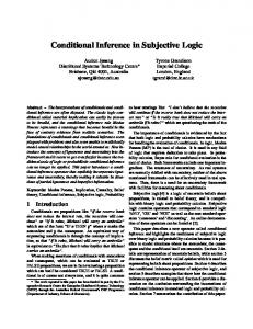
The parameter vector β = (β0 , β1 ) is partially identified since only ([Y0 , Y1 ], X) are observed, with P r {Y ∈ [Y0 , Y1 ]} = 1 and Y0 is strictly smaller than Y1 . To illustrate the differences in inference with curved constraints (unique global maximum) vs flat constraints, I use the following designs for conditional distributions of interval outcome, [Y0 , Y1 ]. Design 1: X is uniformly distributed on [−0.28, 1.12]. Given X = x, Y0 and Y1 are generated as Y0 = 5x − 4(x − 1/2)2 + ε and Y1 = 2 + 5x + 4(x − 1/2)2 + ε, where ε ∼ N (0, 1) and is independent of X. The identified set is given by ΘI = {β ∈ Θ : E[Y0 |X = x] ≤ β0 + β1 x ≤ E[Y0 |X = x] for any x ∈ [0, 1]} .

(4.1)

Figure 1. Design 2: X is uniformly distributed on [0, 1]. Given X = x, Y0 and Y1 are generated as Y0 = 1/2 + 3x + ε and Y1 = 2 + 7x + ε, where ε ∼ N (0, 1) and is independent of X. The identified set in this case is also given by (4.1). Figure 2. The confidence sets proposed in the paper are based on pointwise testing procedure. Therefore, to evaluate the performance of the inference procedures proposed in the paper, I first need to choose a number of points in the parameter space. Corollaries 3.4, 3.6 and 3.10 suggest that any point in the identified set will be covered with a probability that is no less than the desired coverage level 1 − α, In particular, for any point in the interior of the identified set, the coverage probability converges to one, while for some (or all) points on the boundary of the identified set, the coverage probability converges to 1 − α. Finally, the coverage probability for points outside the identified set converges to zero. Therefore, for each design I present simulation results for the set of parameter values that include points on the boundary of the identified set, points in the interior of the identified set, and points that do not belong to the identified set. In both designs, only one out of two constraints can be binding, so we do not need to estimate the number of binding constraints. Finally, for both designs, I consider the number of observation n = {100, 500, 1000} and confidence level 1 − α = {0.75, 0.85, 0.95}.

27

I take independent draws of xi

from the corresponding uniform distribution, and εi ∼ N (0, 1) to simulated the data {([y0,i , y1,i ], xi )}ni=1 . The number of Monte Carlo replications is 1000, number of bootstrap samples is 500.

4.1

Design 1

In the setup of the Design 1, corresponding conditional moment inequalities have a unique global maximum. Therefore, I use inferential procedure described in Section 3.1, which is based on the Normal limiting distribution. In order to estimate conditional moment constraints, the bandwidth h = 1.7n−1/6.5 and a second order kernel K(u) = (15/32)(7u4 − 10u2 + 3)I(|u| ≤ 1) are used. Table 4.1 presents empirical coverage probabilities for different points in the parameter space. Here β = (−3/4, 7) belongs to the boundary of the identified set, while β = (−1/2, 7) is a point in the interior of the identified set. Points β = (−1, 7) and β = (−5/4, 5) do not belong to the identified set, but while the line y = −1 + 7x crosses the lower conditional moment constraint E[Y0 |x] = 5x − 4(x − 1/2)2 ), the line y = −5/4 + 5x lies completely outside the area between upper and lower conditional moment constraints. The parameter value β = (−1, 9) belongs to the boundary of the identified set. However, in a contrast to assumption (S1), the distance between the line y = −1 + 9x and the lower conditional moment constraint is minimized (and equal to zero) at the boundary of the set [0, 1]. Still, as one can see from Table 4.1, the proposed inferential procedure still provides satisfactory results in this case. Table 4.1: Coverage probability for β Coverage Sample size

0.75 100

500

0.85 1000

100

500

0.95 1000

100

500

1000

Asymptotic approximation β = (−3/4, 7)

0.8870

0.8255

0.7640

0.9305

0.8965

0.8425

0.9700

0.9625

0.9435

β = (−1/2, 7)

0.9965

1.0000

1.0000

0.9985

1.0000

1.0000

1.0000

1.0000

1.0000

β = (−1, 7)

0.2870

0.0080

0.0000

0.4120

0.0145

0.0005

0.6185

0.0580

0.0010

β = (−1, 9)

0.5705

0.6645

0.6985

0.6775

0.7865

0.8280

0.8175

0.9215

0.9405

β = (−5/4, 5)

0.0000

0.0000

0.0000

0.0000

0.0000

0.0000

0.0000

0.0000

0.0000

an = n/5

0.4605

0.3290

0.5415

0.6150

0.3840

0.7035

0.6515

0.4460

0.8650

an = n/7

0.5495

0.2350

0.4005

0.5910

0.1965

0.5095

0.5985

0.3235

0.6260

an = n/10

0.5370

0.2120

0.2335

0.5345

0.1925

0.2295

0.5290

0.5260

0.2990

Subsampling approximation, β = (−3/4, 7)

28

4.2

Design 2

In the setup of Design 2, conditional moment constraints are linear functions of x, and therefore there is a continuum of points that maximize conditional moment inequalities. Hence, the inference procedure for this case is based on bootstrap approximation. To estimate conditional moment constraints, I use the bandwidth h = n−1/4.5 and kernel function K(u) = (15/16)(1 − u2 )I(|u| ≤ 1). Table 4.2 shows the empirical coverage for a set of point in the parameter space. In particular, points β = (2, 7) and β = (1/2, 3) belong to the boundary of the identified set with constraints are binding everywhere on [0, 1] . Point β = (2, 5) also belongs to the boundary of the identified set, but constraints are binding in a single point on the boundary of [0, 1]. Finally, points β = (−1/2, 8) and β = (2, 15/2) do not belong to the identified set. The difference is that the line with y = −1/2 + 8x crosses the area between upper and lower constraints, while the line y = 2 + (15/2)x lies completely outside this area. Table 4.2: Coverage probability for β Coverage Sample size

0.75 100

500

0.85 1000

100

500

0.95 1000

100

500

1000

Bootstrap approximation β = (2, 7)

0.6645

0.6150

0.6160

0.8230

0.7640

0.7615

0.9630

0.9440

0.9445

β = (1/2, 3)

0.5385

0.5940

0.6310

0.7235

0.7575

0.7915

0.9430

0.9410

0.9485

β = (2, 5)

0.9915

0.9990

1.0000

0.9970

1.0000

1.0000

0.9995

1.0000

1.0000

β = (1, 5)

1.0000

1.0000

1.0000

1.0000

1.0000

1.0000

1.0000

1.0000

1.0000

β = (−1/2, 8)

0.2220

0.0000

0.0000

0.3695

0.0003

0.0000

0.6925

0.0050

0.0000

β = (2, 15/2)

0.0160

0.0000

0.0000

0.0460

0.0000

0.0000

0.2315

0.0000

0.0000

Subsampling approximation, β = (2, 7) m = n/5

0.8310

0.7480

0.7380

0.9470

0.8920

0.8795

0.9950

0.9860

0.9830

m = n/7

0.8440

0.7365

0.7165

0.9525

0.8735

0.8620

0.9970

0.9800

0.9765

m = n/10

0.8650

0.7255

0.6625

0.9715

0.8655

0.8365

1.0000

0.9835

0.9685

β = (5/4, 2)

0.9215

0.9575

0.9820

0.9665

0.9760

0.9800

0.9960

0.9970

0.9970

Finally, Table 4.3 illustrates “misspecified” case, when inference procedure that is based on the assumption that the conditional moment constraints can have flat parts is applied to the data generated by the model with non-flat constraints (Design 1), and when inference procedure that is based on the assumption that the conditional moment constraints can have unique binding points is applied to the data generated by the model with flat constraints (Design 2). Here we see that bootstrap approximation overcovers in small samples if constraints are non-flat, while the asymptotic approximation 29

severely undercovers when constraints are flat. Moreover, in the case of asymptotic approximation with flat constraints leads to inconsistent inference asymptotically. Table 4.3: ”Misspecified” models Coverage Sample size

0.75 100

500

0.85 1000

100

500

0.95 1000

100

500

1000

0.8205

0.7975

0.7780

0.9960

0.9970

0.9970

Design 2, but normal approximation is used. β = (2, 7)

0.4120

0.3700

0.3220

0.5885

0.5395

0.5165

Design 1, but bootstrap approximation is used β = (−3/4, 7)

5

0.9360

0.9640

0.9820

0.9890

0.9960

0.9940

Conclusion

In this paper I present an approach to constructing confidence sets for each element of partially identified parameters defined by the finite number of conditional moment inequalities. The paper goes beyond the assumption that the conditioning covariates are discrete, and introduces inference procedure applicable in the case where the identified set of the parameter values is defined by a number of conditional moment inequalities with continuously distributed covariates. The inference procedure is based on the supremum statistic for a Nadaraya-Watson estimator of the conditional moment functions that define the set of constraints. I consider three main scenarios and provide a way to construct confidence sets in each of the scenarios: no restrictions on the conditional moment functions; conditional moment functions have unique maximums; conditional moment functions are specified parametrically. Using Monte Carlo simulations I show that in small samples ignoring the shape of the constraints may lead to a conservative coverage for each element of the identified set. I also show that in small samples confidence sets based on subsampling approximation may result in significant undercoverage when conditional moment functions on the boundary of the identified set have peaks. If the researcher is willing to assume that conditional moment functions have unique maximums for the parameter values on the boundary of the identified set, I show that the problem essentially reduces to the problem with finite number of inequalities, evaluated at certain point (estimates of the location of the maximum) and one can use an analog of the Generalized Moment Selection method of Andrews and Soares (2007) to construct confidence sets. Finally, using Monte Carlo simulations, I show that in small samples there is a trade-off between 30

coverage and assumptions about the shape of the constraints. The findings of this paper leave open several questions. Our Monte Carlo exercise shows that in small samples the coverage of confidence sets based on a subsampling approximation is greatly affected by the shape of conditional moment functions that define the constraints. This finding can be explained by an observation that if conditional moment functions have peaks, the behavior of the supremum statistic will be mostly determined by the observations in the small neighborhood of the peak. Therefore, with small sample sizes subsampling approximation may fail to capture this behavior due to insufficient number of observation around the location of the peak. This observation is also relevant for the confidence sets proposed in Kim (2008). It would be of interest to see to what extent the approach proposed by Kim suffers the same drawback. Another interesting question would be to investigate to what extent transforming conditional inequalities into a finite number of unconditional inequalities affects the trade-off between the size of the identified set in this case and the size of the confidence sets. In general, when transforming conditional inequalities into unconditional ones we loose some information, which leads to a larger identified set. However, in small samples confidence set for the “unconditional” identified set based on parametric estimation of unconditional moments can be expected to be tighter than confidence sets for the “conditional” identified set based on nonparametric estimation of conditional moment functions.

6

Appendix

Notation: let {(Y1i , Y2i , Xi ), i = 1, . . . , n} be an i.i.d. sample. Define f (x) marginal density of X µj (x) = E(Yj |X = x), j ∈ J µ ˆj (x) estimator of µj (x) σj2 (x) = E((Yj − µj (x))2 |X = x) σ ˆj2 (x) estimator of σj2 (x) xj0 = arg max µj (x) x∈X

31

xˆj0 = arg max µ ˆj (x) x∈X

cK =

R

K 2 (u)du

Kh (u) = h1 K(u/h)

Proofof Lemma 3.1. For any fixed θ ∈ Θ any constant q, the event I , any j ∈ J and  bn [mj (Z,θ)|X=x]−E[mj (Z,θ)|X=x] bn [mj (Z,θ)|X=x] E E A1 = maxj ≤ c implies A2 = max ≤c sj (x,θ) sj (x,θ) x∈X

x∈V

since if θ ∈ ΘI , then E[mj (Z, θ)|X = x]  ≤ 0. Therefore, for any q the event A01 =  b [m (Z,θ)|X=x]−E[mj (Z,θ)|X=x] E max maxj n j ≤ q implies event A02 = {Tn (θ) ≤ q}. So, for sj (x;θ) j∈J x∈V

any θ ∈ ΘI , ( P {Tn (θ) ≤ qn,1−α } ≥ P

bn [mj (Z, θ)|X = x] − E[mj (Z, θ)|X = x] E max maxj ≤ qn,1−α j∈J x∈V sj (x; θ)

)

where the latter probability is equal to (1 − α) by definition of the quantity qn,1−α . This concludes the proof.2 Proof of Theorem 3.2.

Suppose first that the collection of sets {Vb0j (θ), j ∈

J} is known. For any k-dimensional vector t, consider Wn (x, θ) = P Ebn [mj (Zi ;θ)|Xi =x]−E[mj (Zi ;θ)|Xi =x] . We can use lemmas A.2-A.6 in Johnston (1982) tj sj (x;θ) j∈J

to show that under the assumptions of Theorem 3.2 there exists a sequence of stationary mean zero Gaussian processes with continuous sample paths {Γn (x, θ), n ∈ N} such that sup |Wn (x, θ) − Γn (x, θ)| = op ((log n)−1/2 ). Since the choice of vector t was arbix∈X

trary, there exists a sequence of k-dimensional stationary mean-zero Gaussian processes en (x, θ), n ∈ N} such that {Γ

E

b [m (Z ; θ)|X = x] − E[m (Z ; θ)|X = x]

n j i i j i i ej,n (x, θ) sup −Γ

= op ((log n)−1/2 )

s (x; θ) x∈X ,j∈J j Observe that the functional M (g) = max{maxj gj (x), j ∈ J} is Lipschitz continuous on x∈V

C(X ). Therefore, we can approximate the distribution of bn [mj (Z, θ)|X = x] − E[mj (Z, θ)|X = x] E sj (x; θ) x∈V0 (θ)

Qn (θ) = max max j j∈J

32

,

)

(

  en (·, θ) = max by the distribution of M Γ

max Γj,n (x, θ), j ∈ J . In the case k = 1

x∈V0j (θ)

the distribution of this random variable is known to converge to the extreme value type I distribution, although the rate of convergence is slow (see Hall 1979, 1991). We can use result in Hall (1993) to show that one can approximate distribution of M (Γ n (·, θ)) n n oo by the bootstrap distribution. I will now prove that P lim inf Vεj (θ) ⊆ Vb0j (θ) = 1, n→∞

where Vεj (θ) =({x ∈ X : |E[mj (Z, θ)|X = x]| ≤ ε}. The event ( max j

x∈V0 (θ)

max

|Ebn [mj (Z,θ)|X=x]−0| sj (x,θ)

x∈V0j (θ)

|Ebn [mj (Z,θ)|X=x]−ε| sj (x,θ)

)

ε


0 everywhere on X Let x0 , x00 be two distinct points in X . Then  p

µ ˆ1 (x0 ) − µ1 (x0 )



  0 0  µ ˆ (x ) − µ (x ) 2 2 d → N (0, Σ), nhn  µ 00 00   ˆ1 (x ) − µ1 (x ) µ ˆ2 (x00 ) − µ2 (x00 )

where Σ is a symmetric 4 × 4 matrix with Σ11 = cK σ12 (x0 )/f (x0 ), Σ22 = cK σ22 (x0 )/f (x0 ); Σ33 = cK σ12 (x00 )/f (x00 ), Σ44 = cK σ22 (x00 )/f (x00 ); Σ12 = cK (E[Y1 · Y2 |X = x0 ] − µ1 (x0 )µ2 (x0 )) /f (x0 ); Σ13 = Σ14 = Σ23 = 0; Σ34 = cK (E[Y1 · Y2 |X = x00 ] − µ1 (x00 )µ2 (x00 )) /f (x00 ). Finally, if K is a third order kernel, then we can obtain the above asymptotic result under nh7n → λ2 ≥ 0 and nh5n → ∞ as n → ∞. Proof: To prove joint asymptotic normality, I will employ the Cram´er-Wold device. Therefore, let t = (t1 , t2 , t3 , t4 ) be an arbitrary vector. I will show that random variable ξn =t1 (ˆ µ1 (x0 ) − µ1 (x0 )) + t2 (ˆ µ2 (x0 ) − µ2 (x0 )) + t3 (ˆ µ1 (x00 ) − µ1 (x00 )) + t4 (ˆ µ2 (x00 ) − µ2 (x00 ))

(6.1)

is asymptotically normally distributed with zero mean. Following H¨ardle (1992), for a fixed x define rˆj (x) = µ ˆj (x)fˆ(x). It can be written n P as rˆj (x) = n−1 Yji Khn (x − Xi ). For any x, we have i=1

(ˆ µj (x) − µj (x)) −


rˆj (x) − µj (x)fˆ(x) = op (nhn )−1/2 f (x)

34

Define random variable rˆ1 (x0 ) − µ1 (x0 )fˆ0 (x) rˆ2 (x00 ) − µ2 (x00 )fˆ(x0 ) + t 2 f (x0 ) f (x0 ) rˆ2 (x00 ) − µ2 (x00 )fˆ(x00 ) rˆ1 (x00 ) − µ1 (x00 )fˆ(x00 ) + t + t3 4 f (x00 ) f (x00 )

ζn =t1

(6.2)

Then |(nhn )1/2 (ξn − ζn )| = op (1). For each x and j ∈ J have the following expression for

rˆj (x)−µj (x)fˆ(x) : f (x)

n rˆj (x) − µj (x)fˆ(x) 1 1X = Khn (x − Xi )(Yji − µj (x)) f (x) f (x) n i=1 0

00

For each x ∈ {x , x } and j ∈ J, the bias E



rˆj (x)−µj (x)fˆ(x) f (x)



= O(h2n ), so that

E((nhn )1/2 ζn ) = O(nh5n ). Therefore, E((nhn )1/2 ζn ) = o(1) by condition (1) of the lemma. Condition (4) of the lemma ensures that Lindeberg condition is satisfied for the triangular array {(nhn )1/2 ζn }, which allows to apply Liapunov’s central limit theorem to {(nhn )1/2 ζn }. This implies, together with zero asymptotic bias of {(nhn )1/2 ζn }, that d

(nhn )1/2 ξn → N (0, σξ (t)) for any vector t. Thus, the Cram´er-Wold device warrants joint normal distribution of random vector (nhn )1/2 (ˆ µ1 (x0 ) − µ1 (x0 ), µ ˆ2 (x0 ) − µ2 (x0 ), µ ˆ1 (x00 ) − µ1 (x00 ), µ ˆ2 (x00 ) − µ2 (x00 )). It only remains to derive the asymptotic variance-covariance matrix. I will do this only for Σ12 , since the proof for any other element of matrix Σ is similar. Given joint asymptotic normality, Σ12 is equal to Σ12 = lim nhn E [(ˆ µ1 (x0 ) − µ1 (x0 ))(ˆ µ2 (x0 ) − µ2 (x0 ))] n→∞

n

nhn  h 1 X = lim Khn (x0 − Xi )(Y1i − µ(x0 ))× E n→∞ f (x0 )2 n i=1 n i
 1X 0 0 −1 × Khn (x − Xi )(Y2i − µ(x )) + o (nh) n i=1

35

(6.3)

Finally, " n #   0 n X  x0 − Xi  X 1 x − Xi 0 0 lim E (Y1i − µ(x )) (Y2i − µ(x )) K K n→∞ nhn hn hn i=1 i=1 = cK f (x0 ) [E(Y1 Y2 |X = x0 ) − µ1 (x0 )µ2 (x0 )] The last statement of the lemma follows from the expression of the bias for the higher order kernels. This concludes the proof of the lemma. 2 Next lemma shows consistency and asymptotic normality of kernel estimator of a unique maximum and provides a simplified version of the proof in Ziegler (2000), since here we are not interested in asymptotic normality of the estimator of the location of the maximum. This allows to relax assumptions about the choice of bandwidth. Here for the ease of the presentation I omit index j in µj , σj and xj0 . Lemma 6.2 Let the equivalent of conditions (A1)-(A3), (R1)-(R3) and (UM1)-(UM3) hold for i.i.d. sample {(Yi , Xi ), i = 1, . . . , n} and µ(x) = E(Y |X = x). Let x0 = arg max µ(x) and xˆ0 = arg max µ ˆ(x). Suppose that 1. nh7 → λ2 ≥ 0 and nh5 → ∞ as n → ∞; 2. K is a symmetric, twice continuously differentiable third order kernel that vanishes outside the interval [−1, 1]. Then

√

d

nh(ˆ µ(ˆ x0 ) − µ(x0 )) → N (0, ω)

where ω = cK (E(Y 2 |X = x0 ) − µ2 (x0 ))/f (x0 ). Proof: We can write µ ˆ(ˆ x0 ) − µ(x0 ) = (ˆ µ(ˆ x0 ) − µ ˆ(x0 )) + (ˆ µ(x0 ) − µ(x0 )) d

Lemma 6.1 implies that under our assumptions, (nh)1/2 (ˆ µ(x0 ) − µ(x0 )) → N (0, ω). It remains to show that (nh)1/2 (ˆ µ(ˆ x0 ) − µ ˆ(x0 )) = op (1). Since X is compact and µ(·) is continuous on X , then by Heine-Cantor theorem µ(·) is also uniformly continuous on X . Together with the assumptions of the lemma 36

it implies is uniform consistency of kernel estimator µ ˆ(x) on X (see Bierens, 1987). Therefore p

sup |ˆ µ(x) − µ(x)| → 0 as n → ∞ x∈X p

This in turn implies that kˆ x0 − x0 k → 0. So, xˆ0 is a consistent estimator for x0 . By Taylor series expansion of µ ˆ(x0 ) around x = xˆ0 we have µ ˆ(ˆ x0 ) − µ ˆ(x0 ) =

∂µ ˆ(ˆ x0 ) (x0 − xˆ0 ) + Op (kx0 − xˆ0 k2 ), ∂x

where the last term follows from the fact that Hessian of µ ˆ(x0 ) is bounded with probability 1, since as nh5 → ∞ the second derivative of µ ˆ(x) evaluated at x = x0 is a consistent estimator of the second derivative of µ(x) evaluated at x = x0 . By the construction of xˆ0 , we have

∂µ ˆ(ˆ x0 ) ∂x

= 0, so that µ ˆ(ˆ x0 )− µ ˆ(x0 ) = Op (kx0 − xˆ0 k2 ). Therefore, in

order to evaluate the term (nh)1/2 (ˆ µ(ˆ x0 ) − µ ˆ(x0 )) we need to find a rate of convergence of xˆ0 . Exact Taylor series expansion of first order conditions for xˆ0 around x = x0 gives us 0=

∂µ ˆ(xn ) ∂µ ˆ(x0 ) ∂ 2 µ ˆ(˜ x) = + (x0 − xn ), ∂x ∂x ∂x∂x0

where x˜ lies between x0 and xˆ0 and therefore k˜ x −x0 k = op (1). Provided that nh5 → ∞, we have

∂ 2µ ˆ(x0 ) ∂ 2 µ(x0 ) − = op (1) ∂x∂x0 ∂x∂x0

Continuity of the second derivative of µ(·) in the neighborhood of x0 (assumption (UM2)) implies that also ˆ(˜ x) ∂ 2 µ(x0 ) ∂ 2µ − = op (1) ∂x∂x0 ∂x∂x0 By assumption (UM2),

∂ 2 µ(x0 ) ∂x∂x0

is negative definite, therefore its inverse exists and we

can write  (ˆ x0 − x0 ) = Since nh3 → 0, then 7

2

nh → λ , then

(x0 ) k ∂ µˆ∂x

−

2

∂ µ(x0 ) ∂x∂x0

−1

! + op (1)

∂µ ˆ(x0 ) ∂x

∂µ ˆ(x0 ) 0) is a consistent estimator of ∂µ(x . ∂x ∂x ∂µ(x0 ) 3 −1 k = Op ((nh ) ). By definition, x0 ∂x

37

Moreover, since is the argmax of

µ(x) and it belongs to the interior of X , so by assumption (UM3) we have ∂µ(x0 ) =0 ∂x

(6.4)

This that kˆ x0 − x0 k = Op ((nh3 )−1 ). Therefore, (nh)1/2 (ˆ µ(ˆ x0 ) − µ ˆ(x0 )) =  implies  1/2 Op (nh) = Op (n−3/2 h−11/2 ) = op (1) since nh5 → ∞. This completes the proof of n2 h6 the lemma. 2 Theorem 3.2 immediately follows from Lemmas 6.1 and 6.2 and the fact that K is a third order kernel. 2 Lemma 6.1 also provides a consistent estimator of variance-covariance matrix Σ(θ).   b Lemma 6.3 (Estimator of Σ(θ)) For any j, l ∈ {1, 2}, Σ(θ) given by jl



b Σ(θ)

n

 jl

1 X  nh j j b = Kh (ˆ x0 − Xi )(mj (Zi , θ) − En [mj (Zi , θ)|X = xˆ0 ] × fˆ(ˆ xj )fˆ(ˆ xl ) n 0

×

n 1 X

n

0

i=1

 bn [ml (Zi , θ)|X = xˆl0 ]) Kh (ˆ xl0 − Xi )(ml (Zi , θ) − E

i=1

is a consistent estimator of (Σ(θ))jl . Proof of Theorem 3.4. We need to show that Gr,n (θ) and Ten (θ) have the same limiting distribution if θ belongs to the identified set ΘI . Asymptotic distribution of Ten (θ) follows from Theorem 3.3, so it remains to show that Gr,n (θ) converges in distribution to the same functional of multivariate Gaussian random variable with variance-covariance bn [mj (Z, θ)|X = x], xˆj0 , Σ(θ), b matrix Σ(θ). This follows from consistency of estimators E and a law of iterated logarithm for kernel estimator (see H¨ardle, 1984), which implies that for any θ ∈ ΘI and our choice of a sequence {τn , n = 1, . . .} we have ( P

( lim 1

n→∞

bn [m(Zi , θ)|Xi = xˆj0 (θ)] E ≥ −τn sj (ˆ xj0 (θ), θ)

)

) = 1 E[mj (Zi , θ)|Xi = xj0 (θ)] = 0 

=1

This completes the proof. 2 Proof of Theorem 3.5. The second part of the claim follows directly from Theorem 3.1 in Shapiro (2000). It only remains to show that if function f (x, β) satisfies the 38

√ d conditions of Theorem 3.5 and n(βˆn −β) → N (0, Σβ ), then stochastic process Zn (x) = √ ˆ − f (x, β)) can be approximated by a stationary Gaussian process Z∞ (x) n(f (x, β) with continuous sample paths. For a fixed x, Delta method implies that √

∂f (x, b) ˆ n(f (x, β) − f (x, β)) = N (0, Σβ ) + op (1) ∂b b=β

(6.5)



∂f (x,b) ∂b

Define Z∞ (x) = N (0, Σβ ). Then Z∞ (x) has continuous sample paths since b=β ∂f (x,b) is continuous on X and sup |Zn (x) − Z∞ (x)| = op (1). This concludes the ∂b b=β

proof. 2

x∈X

References [1] Andrews, D.W.K., S. Berry, and P. Jia (2004). “Confidence Regions for Parameters in Discrete Games with Multiple Equilibria, with an Application to Discount Chain Store Location,” working paper, Yale University. [2] Andrews, D.W.K. and P. Guggenberger (2007). “Validity of Subsampling and Plug-in Asymptotic Inference for Parameters Defined by Moment Inequalities,” working paper, Yale University. [3] Andrews, D.W.K. and X. Shi (2009). “Inference for Parameters De.ned by Conditional Moment Inequalities,” working paper, Yale University. [4] Andrews, D.W.K. and G. Soares (2007). “Inference for Parameters Defined by Moment Inequalities Using Generalized Moment Selection,” working paper, Yale University. [5] Beresteanu, A. and F. Molinari (2007). “Asymptotic Properties for a Class of Partially Identified Models,” working paper, Cornell University [6] Berman, S.M. (1980). “A Compound Poisson Limit for Stationary Sums, and Sojourns of Gaussian Processes,” The Annals of Probability, 8(3), 511-538. [7] Bierens, H.J. (1987). “Kernel Estimators of Regression Functions,” Ch. 3 in T.F. Bewley (ed.), Advances in Econometrics, Cambridge University Press, Vol. I, 99-144.

39

[8] Birke, M., and H. Dette (2007). “Testing Strict Monotonicity in Nonparametric Regression,” Mathematical Methods of Statistics, 16(2), 110-123. [9] Bowman, A.V., M. C. Jones, and I. Gijbels (1998). “Testing monotonicity of regression,” Journal of Computational and Graphical Statistics, 7, 489-500. [10] Bugni, F. (2007). “Bootstrap Inference for Partially Identified Models,” Working paper, Northwestern University. [11] Canay, I. (2007). “EL Inference for Partially Identified Models: Large Deviations Optimality and Bootstrap Validity,” Working paper, University of Wisconsin Madison. [12] Chernozhukov, V., H. Hong, and E. Tamer (2007). “Parameter Set Inference in a Class of Econometric Models. Econometrica, 75(5), 1243-1284. [13] Chernozhukov, V., S. Lee, and A.M. Rosen (2009). “Intersection Bounds: Estimation and Inference,” CEMMAP working paper CWP19/09. [14] D¨ umbgen, L. and V.G. Spokoiny. “Multiscale Testing of Qualitative Hypotheses,” The Annals of Statistics, 29(1), 124-152. [15] Fan, Y. and S. Park (2007). “Confidence Sets for Some Partially Identified Parameters,” working paper, Vanderbilt University. [16] Galichon, A. and M. Henry (2006). “Dilation Bootstrap: A Natural Approach to Inference in Incomplete Models,” working paper. [17] Ghosal, A., A. Sen, and A.W. van der Vaart (2000). “Testing Monotonicity of Regression,” The Annals of Statistics, 28(4), 1054-1082. [18] Hall, P. (1979) “On the Rate of Convergence of Normal Extremes,” Journal of Applied Probability, 16, 433-439. [19] Hall, P. (1991). “On Convergence Rates of Suprema,” Probability Theory Related Fields, 89, 447-455. [20] Hall, P. (1993). “On Edgeworth Expansion and Bootstrap Confidence Bands in Nonparametric Curve Estimation,” Journal of the Royal Statistical Society, Series B (Methodological), 55(1), 291-304. [21] H¨ardle, W. (1984). “A Law of the Iterated Logarithm for Nonparametric Regression Function Estimators,” The Annals of Statistics, 12(2), 624-635. 40

[22] H¨ardle, W. (1992). Applied Nonparametric Regression. New York: Cambridge University Press. [23] Horowitz, J.L. and C.F. Manski (2000). “Nonparametric Analysis of Randomized Experiments with Missing Covariate and Outcome Data,” Journal of the American Statistical Association, 95(449), 77-84. [24] Imbens, G.W. and C.F. Manski (2004). “Confidence Intervals for Partially Identified Parameters,” Econometrica, 72(6), 1845-1857. [25] Johnston, G.J. (1982). “Probabilities of Maximal Deviations for Nonparametric Regression Function Estimates,” Journal of Multivariate Analysis, 12, 402-414. [26] Juditsky, A. and A. Nemirovski (2002). “On Nonparametric Tests of Positivity/Monotonicity/Convexity,” The Annals of Statistics, 30(2), 498-527. [27] Khan, S. and E. Tamer (2007). “Inference on Randomly Censored Regression Models Using Conditional Moment Inequalities,” working paper. [28] Kim, K. (2009). “Set Estimation and Inference with Models Characterized by Conditional Moment Inequalities,” working paper, University of Minnesota. [29] Konakov, V.D. and V.I. Piterbarg (1984). “On the Convergence Rate of Maximal Deviation Distribution for Kernel Regression Estimates,” Journal of Multivariate Analysis, 15, 279-294. [30] Lee, S., O. Linton, and Y. Whang (2007). “Testing for Stochastic Monotonicity,” working paper. [31] Liao, Y., and W. Jiang (2008). “Bayesian Analysis in Moment Inequality Models,” working paper, Northwestern University. [32] Manski, C.F. and E. Tamer (2002). “Inference on Regressions with Interval Data on a Regressor or Outcome,” Econometrica, 70(2), 519-546. [33] Manski, C.F. (2003). Partial Identification of Probability Distributions. SpringerVerlag, New York. [34] Menzel, K. (2009) “Estimation and Inference with Many Moment Inequalities,” working paper. [35] Moon, H.R. and F. Schorfheide (2007). “A Bayesian Look at Partially-Identified Models,” working paper, University of Pennsylvania. 41

[36] Pakes, A., J. Porter, K. Ho, and J. Ishii (2005). “Moment Inequalities and Their Application,” working paper. [37] Romano, J.P. and A.M. Shaikh (2006). “Inference for the Identified Set in Partially Identified Econometric Models,” working paper. [38] Romano, J.P. and A.M. Shaikh (2007). “Inference for Identifiable Parameters in Partially Identified Econometric Models,” working paper. [39] Rosen, A.M. (2006). “Confidence Sets for Partially Identified Parameters that Satisfy a Finite Number of Moment Inequalities,” working paper, University College London. [40] Shapiro, A. (2000). “Statistical Inference of Stochastic Optimization Problems,” in S. P. Uryasev (ed.), Probablistic Constrained Optimization: Methodology and Applications, Kluwer Academic Publishers, 282-304. [41] Stoye, J. (2007). “More on Confidence Intervals for Partially Identified Parameters,” working paper, NYU. [42] Tamer, E. (2003). Incomplete simultaneous discrete response model with multiple equilibria, Review of Economic Studies, 70(1), 147-165. [43] Ullah, A. and A. Pagan (1999). Nonparametric econometrics. Cambridge University Press. [44] Wu, C.F.Y. (1986). “Jacknife, Bootstrap and Other Resampling Methods in Regression Analysis,” Annals of Statistics, 14, 1261-1350. [45] Ziegler, K. (2000). “Nonparametric Estimation of Location and Size of Maxima of Regression Functions in the Random Design Case Based on the NadarayaWatson Estimator with Data-Dependent Bandwidths,” Habilitation Thesis. [46] Ziegler, K. (2003). “On the Asymptotic Normality of Kernel Regression Estimators of the Mode in the Random Design Model,” Journal of Statistical Planning and Inference, 115, 123-144.

42

Figure 1: Both flat and non-flat constraints. This figure illustrates the case where E(Y1 |x) is linear in x, while E(Y0 |x) is nonlinear. Therefore, there exists some θ0 in the identified set ΘI such that θ00 +θ10 ·x−E(Y1 |x) < 0 and E(Y0 |x)−θ00 −θ10 ·x = 0 for all x ∈ [0, 1]. There also exist some θ00 in the identified set ΘI such that E(Y0 |x)−θ000 −θ100 ·x < 0 and θ000 + θ100 · x − E(Y1 |x) ≤ 0 for any x ∈ [0, 1], and θ000 + θ100 · x0 − E(Y1 |x0 ) = 0 for some x0 ∈ [0, 1]. In this case the bootstrap method will give conservative coverage for θ00 even though it belongs to the boundary of the identified set.

43

Figure 2: Both constrains are non-flat. This figure illustrates the case where both E(Y1 |x) and E(Y0 |x) are nonlinear. In this case method based on critical values obtained from the bootstrap approximation gives conservative coverage for any point on the boundary of the identified set. In contrast, method based on the Gaussian approximation provides the coverage that has asymptotically exact size.

44