Infinite Runs in Weighted Timed Automata with Energy Constraints

Infinite Runs in Weighted Timed Automata with Energy Constraints Patricia Bouyer1? , Uli Fahrenberg2 , Kim G. Larsen2 , Nicolas Markey1? , and Jiˇr´ı Srba2?? 1

Lab. Spécification et Vérification, CNRS & ENS Cachan, France {bouyer,markey}@lsv.ens-cachan.fr 2 Dept. of Computer Science, Aalborg University, Denmark {uli,kgl,srba}@cs.aau.dk

Abstract. We study the problems of existence and construction of infinite schedules for finite weighted automata and one-clock weighted timed automata, subject to boundary constraints on the accumulated weight. More specifically, we consider automata equipped with positive and negative weights on transitions and locations, corresponding to the production and consumption of some resource (e.g. energy). We ask the question whether there exists an infinite path for which the accumulated weight for any finite prefix satisfies certain constraints (e.g. remains between 0 and some given upper-bound). We also consider a game version of the above, where certain transitions may be uncontrollable.

1

Introduction

The overall motivation of the research underlying this paper is the quest of developing weighted (or priced) timed automata and games [3, 2] into a universal formalism useful for formulating and solving a broad range of resource scheduling problems of importance in application areas such as, e.g., embedded systems. In this paper we introduce and study a new resource scheduling problem, namely that of constructing infinite schedules or strategies subject to boundary constraints on the accumulation of resources. More specifically, we propose finite and timed automata and games equipped with positive as well as negative weights, respectively weight-rates. With this extension, we may model systems where resources are not only consumed but also occasionally produced or regained, e.g. useful in modelling autonomous robots equipped with solar-cells for energyharvesting or with the ability to search for docking-stations when energy-level gets critically low. Main challenges are now to synthesize schedules or strategies that will ensure indefinite safe operation with the additional guarantee that energy will always be available, yet never exceeds a possible maximum storage capacity. ? ??

This author is partially supported by project DOTS (ANR-06-SETI-003). This author is partially supported by grant no. MSM-0021622419.

2

Bouyer, Fahrenberg, Larsen, Markey, Srba

`0

`1

`2

3

−3

+6

−6

2 1

x := 0

a)

x=1

b)

3

3

2

2

1

c)

0 0

1

0

1

1

d)

0 0

1

0

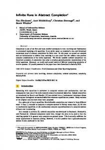
Fig. 1. a) Weighted Timed Automaton (global invariant x ≤ 1). b) U = +∞ and U = 3. c) U = 2. d) U = 1 and W = 1.

As a basic example, consider the weighted timed automaton in Fig. 1a) with infinite behaviours repeatedly delaying in `0 , `1 and `2 for a total of precisely one time-unit. The negative weights (−3 and −6) in `0 and `2 indicate the rates by which energy will be consumed, and the positive rate (+6) in `1 indicates the rate by which energy will be gained. Thus, for a given iteration the effect on the amount of energy remaining will depend highly on the distribution of the one time-unit over the three locations. Let us observe the effect of lower and upper constraints on the energy-level on so-called bang-bang strategies, where the behaviour remains in a given location as long as permitted by the given bounds. Fig. 1b) shows the bang-bang strategy given an initial energy-level of 1 with no upper bound (dashed line) or 3 as upper bound (solid line). In both cases, it may be seen that the bang-bang strategy yields an infinite behaviour. In Fig. 1c) and d), we consider the upper bounds 2 and 1, respectively. For an upper bound of 2, we see that the bang-bang strategy reduces an initial energylevel of 1 12 to 1 (solid line), and yet another iteration will reduce the remaining energy-level to 0. In fact, the bang-bang strategy—and it may be argued, any other strategy—fails to maintain an infinite behaviour for any initial energy-level except for 2 (dashed line). With upper-bound 1, the bang-bang strategy—and any other strategy—fails to complete even one iteration (solid line). We also propose an alternative weak notion of upper bounds, which does not prevent energy-increasing behaviour from proceeding once the upper bound is reached but merely maintains the energy-level at the upper bound. In this case, as also illustrated in Fig. 1d) (dashed line), the bang-bang strategy is quite adequate for yielding an infinite behaviour. In this paper, we ask the question whether some, or all, of the infinite paths obey the property that the weight accumulated in any finite prefix satisfies certain constraints. The lower-bound problem requires the accumulated weight never

Infinite Runs in Weighted Timed Automata with Energy Constraints

3

drop below zero, the interval-bound problem requires the accumulated weight to stay within a given interval, and in the lower-weak-upper-bound problem the accumulated weights may not drop below zero, with the additional feature that the weights never accumulate to more than a given upper bound; any increases above this bound are simply truncated. We also consider a game version of the above setting, where certain transitions may be uncontrollable. For finite weighted automata, we show that the lower- and lower-weak-upperbound problems are decidable in polynomial time. In the game setting we prove these problems to be P-hard but decidable in NP ∩ coNP. The interval-bound problem is on the other hand NP-hard but decidable in PSPACE and in the game setting it is EXPTIME-complete. For one-clock weighted timed automata, the lower- and lower-weak-upper-bound problems remain in P, but the interval-bound problem in the game setting is already undecidable. Related Work. Recently, extensions of timed automata with costs (or prices) to measure quantities like energy, bandwidth, etc. have been introduced and subject to significant research. In these models—so-called priced or weighted timed automata—the cost can be used to measure the performance of a system allowing various optimization problems to be considered. Examples include cost-optimal reachability problem in a single-cost setting [2, 3], as well as in a multi-cost setting [20], or the computation of (mean-cost or discounted) costoptimal infinite schedules [6, 16]. Also games where players try to optimize the cost have been considered [1, 7, 13, 5, 10], and several model-checking problems have been studied [12, 5, 9, 11]. It is worth noticing that in these last frameworks (model-checking and games), most of the problems are undecidable, and they can be solved algorithmically only for the (restricted) class of one-clock automata. However, in the priced extensions considered so far, only non-negative costs are allowed restricting the types of quantities one can measure. The only exception concerns the optimal-cost reachability problem, which has been solved even when negative costs are allowed [4], but the proof is basically not much more involved than with only non-negative costs. In the current work, we pursue this line of research, and focus on non-trivial problems that can be posed on timed automata with arbitrary costs, which allow to model interesting problems on timed systems with (bounded) resources. Due to space limitations, most proofs had to be omitted in this paper. A long version is available as [8].

2 2.1

Models and Problems Weighted Automata and Games

A weighted automaton is a tuple A = (S, s0 , T ) consisting of a set of locations (or states) S, an initial location (state) s0 ∈ S, and a set of transitions T ⊆ S × ×S. p A transition (s, p, s0 ) is customarily denoted s − → s0 , where p ∈ is the weight of that transition. We implicitly consider only non-blocking automata where every location has at least one outgoing transition. If S and T are finite sets and T ⊆ S × × S then A is called a finite weighted automaton.

R

Z

R

4

Bouyer, Fahrenberg, Larsen, Markey, Srba p1

p2

A run in A starting from s ∈ S is a finite or infinite sequence s = s1 −→ s2 −→ s3 −→ · · · . We write Runs(A, s) for the set of all runs in A starting from s. Given a pn−1 p1 finite run γ = s1 −→ · · · −−−→ sn , we write last(γ) to denote its final location sn . p3

R

R

Definition 1. Let A = (S, s0 , T ) be a weighted automaton, c ∈ , b ∈ ∪ {∞}, pn−1 p1 and let γ = s1 −→ · · · −−−→ sn ∈ Runs(A, s1 ). The accumulated weight with initial credit c under weak upper bound b is pc↓b (γ) = rn , where r1 , . . . , rn ∈ are defined inductively by r1 = min(c, b), ri+1 = min(ri + pi , b).

R

So for computing pc↓b (γ), costs are accumulated along the transitions of γ, but only up to a maximum accumulated cost b; possible increases above b are simply discarded. The case b = ∞ is special; we will denote pc (γ) = pc↓∞ (γ) = Pn−1 c + i=1 pi . Also, we will write p(γ) = p0 (γ). A weighted game is a tuple G = (S1 , S2 , s0 , T ) where S1 and S2 are two disjoint sets of locations, and AG = (S1 ∪ S2 , s0 , T ) is a weighted automaton. Note that we only introduce turn-based weighted games here. A run of G is a run of AG , and we write Runs(G) for Runs(AG ). A strategy σ for Player i, where i = 1 or i = 2, maps each finite run γ ending in Si to a transition departing from last(γ). Given a location s in G and a strategy σ for pn−1 p1 p2 Player i, an outcome of σ from s is any run s1 −→ s2 −→ · · · −−−→ sn starting in s pk−1 pk p1 p2 such that for any k, if sk ∈ Si then sk −→ sk+1 = σ(s1 −→ s2 −→ · · · −−−→ sk ). We are now able to formulate the problems which we shall be concerned with. The lower-bound problem: Given a weighted game G and an initial credit c, does there exist a strategy for Player 1 such that any infinite outcome γ from the initial state of G has pc (γ 0 ) ≥ 0 for all finite prefixes γ 0 of γ? The lower-weak-upper-bound problem: Given a weighted game G, a weak upper bound b and an initial credit c ≤ b, does there exist a strategy for Player 1 such that any infinite outcome γ from the initial state of G has pc↓b (γ 0 ) ≥ 0 for all finite prefixes γ 0 of γ? The interval-bound problem: Given a weighted game G, an upper bound b, and an initial credit c ≤ b, does there exist a strategy for Player 1 such that any infinite outcome γ from the initial state of G has 0 ≤ pc (γ 0 ) ≤ b for all finite prefixes γ 0 of γ? Note that by Martin’s determinacy theorem [21], our games are determined : Player 1 has a strategy for winning one of the above games if, and only if, Player 2 does not have a strategy for making Player 1 lose. Special variants of the above problems are obtained when one of the sets S1 and S2 is empty. In case S2 = ∅, they amount to asking for the existence of an infinite path adhering to the given bounds; in case S1 = ∅, one asks whether all infinite paths stay within the bounds. The former problems will be referred to as existential problems, the latter as universal ones. 2.2

The Timed Setting

A weighted timed automaton is a tuple A = (Q, q0 , C, I, E, rate), with Q a finite set of locations, q0 ∈ Q the initial location, C a finite set of clocks, I : Q → Φ(C)


5

location invariants, E ⊆ Q × Φ(C) × 2C × Q a finite set of transitions, and rate : Q → location weight-rates. Here the set Φ(C) of clock constraints ϕ is defined by the grammar ϕ ::= x ./ k | ϕ1 ∧ ϕ2 with x ∈ C, k ∈ and ./ ∈ {≤, , =}. The semantics of a weighted timed automaton A is given by a weighted automaton JAK with states (q, v), where q ∈ Q and v : C → ≥0 , and transitions of two types:

Z

Z

R

R

p

– Delay transitions (q, v) − →t (q, v + t) for some t ∈ ≥0 . Such a transition exists whenever v + t0 |= I(q) for all t0 ∈ [0, t], and its weight is p = t · rate(q). 0 – Switch transitions (q, v) − →e (q 0 , v 0 ), where e = (q, g, r, q 0 ) is a transition of A. Such a switch transition exists whenever v |= g ∧ I(q), v 0 = v[r ← 0], and v 0 |= I(q 0 ). Switch transition have always the weight 0. p1

0

p2

A run of A is a sequence (q1 , v1 ) −→t1 (q1 , v10 ) − →e1 (q2 , v2 ) −→t2 (q2 , v20 ) · · · of alternating delay and switch transitions in JAK. We write Runs(A) for the set of all runs of A. The accumulated weight (with initial credit c and weak upper bound b) for runs of a weighted timed automaton are given by Definition 1. A weighted timed game is a tuple G = (Q, q0 , C, I, E1 , E2 , rate) such that AG = (Q, q0 , C, I, E1 ∪ E2 , rate) is a weighted timed automaton. States and runs of a weighted timed game are those of the underlying weighted timed automaton, and we again write Runs(G) for Runs(AG ). Given a weighted timed game G, a strategy for Player i (i ∈ {1, 2}) is a partial function σ mapping each finite run of Runs(AG ) to Ei ∪ {λ}, where λ ∈ / E1 ∪ E2 is the “wait” action. For a finite run γ ending in (q, v), it is required that if σ(γ) = λ p 0 then (q, v) − →t (q, v + t) for some t > 0, and if σ(γ) = e then (q, v) − →e (q 0 , v 0 ). Given a state s = (q, v) of a weighted timed game G and a strategy σ for Player i, the set Out(σ, s) of outcomes of σ from s is the smallest subset of Runs(G, s) such that – (q, v) is in Out(σ, s); – if γ ∈ Out(σ, s) is a finite run ending in (qn , vn ), then a run of the form γ → (qn+1 , vn+1 ) is in Out(σ, s) if either • (qn , vn ) → − e (qn+1 , vn+1 ) with e ∈ E3−i , • (qn , vn ) → − e (qn+1 , vn+1 ) with e = σ(γ) ∈ Ei , or • (qn , vn ) → − t (qn+1 , vn+1 ) with t ∈ ≥0 , and σ(γ → − t0 (qn , vn + t0 )) = λ for 0 all t ∈ [0, t); – an infinite run is in Out(σ, s) if all its finite prefixes belong to Out(σ, s).

R

A weighted timed game G = (Q, q0 , C, I, E1 , E2 , r) is said to be turn-based if the set of edges leaving any q ∈ Q is a subset of either E1 or E2 . In that case, the semantics of G is a (turn-based, infinite) weighted game as introduced in the previous section. However, weighted timed games introduced above are more general than turn-based ones, and we shall later use the more general notion. For weighted timed games, we will be interested in the same three problems as in the previous section; the existence of a strategy whose outcomes are infinite runs remaining within given bounds. As in the previous section, we have the special cases of existential and universal problems.

6

3


Fixed-Point Characterization

Let us introduce some terminology. For the lower-bound problem, we say that an infinite path γ is c-feasible for some initial credit c < +∞, if pc (γ 0 ) ≥ 0 for all finite prefixes γ 0 of γ, and that γ is feasible if it is c-feasible for some c. Given a weighted game (S1 , S2 , s0 , T ) and b ∈ ≥0 , we define three predicates L, Wb , Ub : S × ≥0 → {tt, ff } to be the respective maximal fixed points to the following equations: ( p s ∈ S1 =⇒ ∃s − → s0 ∈ T : L(s0 , c + p) L(s, c) = 0 ≤ c ∧ p s ∈ S2 =⇒ ∀s − → s0 ∈ T : L(s0 , c + p) ( p s ∈ S1 =⇒ ∃s − → s0 ∈ T : Wb (s0 , max(b, c + p)) Wb (s, c) = 0 ≤ c ≤ b ∧ p s ∈ S2 =⇒ ∀s − → s0 ∈ T : Wb (s0 , max(b, c + p)) ( p s ∈ S1 =⇒ ∃s − → s0 ∈ T : Ub (s0 , c + p) Ub (s, c) = 0 ≤ c ≤ b ∧ p s ∈ S2 =⇒ ∀s − → s0 ∈ T : Ub (s0 , c + p) .

R

R

The right-hand side of each of these equations defines a monotone functional on the power set lattice of S × ≥0 , hence indeed the maximal fixed points exist. Also, if the weighted game under investigation is image finite, i.e. if the sets p {(p, s0 ) | s − → s0 ∈ T } are finite for all states s, then it can be shown that these respective functionals are continuous, implying that the maximal fixed points can be obtained as the limits of the iterated application of the respective functionals to the maximal element S × ≥0 of the power set lattice. The proof of the lemma below is immediate from the definition of the predicates.

R

R

R

Lemma 2. Let (S1 , S2 , s0 , T ) be a weighted game and s ∈ S1 ∪ S2 , b, c ∈ ≥0 . Then (s, c) ∈ L (or (s, c) ∈ Wb , or (s, c) ∈ Ub ) if and only if there exists a strategy for Player 1 such that any infinite path γ from s consistent with the strategy is c-feasible for the lower-bound problem (or lower-weak-upper-bound problem, or interval-bound problem, respectively). For the lower-bound problems, the above fixed-point characterization can be stated in a different way by defining recursively the infimum credits sufficient for feasibility—note that such a notion does not make sense for the interval-bound problem, as here the set of sufficient credits is not necessarily upward-closed. For a given weighted game (S1 , S2 , s0 , T ) and b ∈ ≥0 , let L, Wb : S → ∪ {∞} be the functions defined as respective minimal fixed points to the following equations: ( p min{L(s0 ) − p | s − → s0 } if s ∈ S1 L(s) = p 0 0 max{L(s ) − p | s − → s } if s ∈ S2 ( p min b, min{W (s0 ) − p | s − → s0 } if s ∈ S1 Wb (s) = p min b, max{W (s0 ) − p | s − → s0 } if s ∈ S2 .

R

R


7

3

+3 s0 a)

−1

+1 s1

s0

−3

s1

b)

2 ε 2− 2

2−ε

1

c)

0 0

1

Fig. 2. a), b) Weighted automata with and without feasible paths. c) One fixed-point iteration on the weighted timed automaton of Fig. 1.

Proposition 3. We have L(s, c) if and only if c ≥ L(s), and Wb (s, c) if and only if Wb (s) ≤ c ≤ b. The following lemma shows that for finite weighted games, there is a predescribed upper limit for the values of L and Wb . This implies that the fixed-point computations can be terminated after a finite number of iterations. For timed games, the second part of the next example below shows that this is not necessarily the case.

R

Lemma 4. Let (S1 , S2 , s0 , T ) be a finite weighted game and b ∈ ≥0 . Let M = P p {−p | s − → s0 ∈ T, p < 0}. Then for any state s, L(s) < ∞ if and only if L(s) ≤ M , and Wb (s) < ∞ if and only if Wb (s) ≤ M . Example 5. Consider the weighted automata in Fig. 2a) and 2b). Let us attempt to compute L using iterative application of the recursive definition. For a) we find the following fixed points after two iterations: L(s0 ) = 0 and L(s1 ) = 1. For b) we get the following sequence of decreasing approximations: L2n (s0 ) = L2n+1 (s0 ) = 2n and L2n (s1 ) = L2n−1 (s1 ) = 2n + 1. Hence clearly L(s0 ) = L(s1 ) = ∞, though this fixed point is not reached within a finite number of iteration. In Fig. 2c) we reconsider the weighted timed automaton from Fig. 1 under the interval-bound problem with upper bound 2. If we assume that after n iterations of the fixed-point computation, U2n ((`2 , 1), c) = tt if and only if c ∈ [2 − ε, 2] for some ε, then U2n+1 ((`0 , 0), c) = tt if and only if c ∈ [2 − 12 ε, 2]. The largest fixed point—U2 ((`2 , 1), c) = tt if and only if c = 2—is only reached as the limit of this infinite sequence of approximations. t u

4

Lower-Bound Problems

In this section we treat the lower-bound and lower-weak-upper-bound problems for finite automata, one-clock timed automata, and for finite games. For one-clock timed games, these problems are open. 4.1

Finite Weighted Automata

For a given finite weighted automaton A = (S, s0 , T ), we denote by MinCr(γ), for a path γ in A, the minimum c ≥ 0 for which γ is c-feasible, and by MinCr(s),

8


for a state s ∈ S, the minimum of MinCr(γ) over all feasible paths γ emerging from s. A cycle γ = s0 → s1 → · · · → s0 in A is non-losing if p(γ) ≥ 0 (or equivalently, pc (γ) ≥ c for any initial credit c). A lasso λ from a given state s0 is an infinite path of the form γ1 (γ2 )ω , where γ1 = s0 → s1 → · · · → si−1 , γ2 = si → · · · → sk → si , and si−1 → si are paths in A, and with si 6= sj whenever i = 6 j ≤ k. It is clear that if a lasso γ1 (γ2 )ω constitutes a feasible path then the cycle γ2 must be non-losing. Lemma 6. Let A = (S, s0 , T ) be a finite weighted automaton and s ∈ S. For any feasible path γ from s, there exists a feasible lasso λ also from s such that MinCr(λ) ≤ MinCr(γ). Proof. Let c = MinCr(γ), and assume first that there is a cycle π in γ such that p(π) ≥ 0. Write γ = γ1 πγ2 , then λ = γ1 π ω is a feasible lasso from s, and MinCr(λ) ≤ MinCr(γ). Assume now that there is no cycle π in γ with p(π) ≥ 0. We can write γ = γ1 γ2 , where γ2 only takes transitions that appear infinitely often along γ. As there is no cycle with non-negative weight in γ, the weights of prefixes of γ2 decrease to −∞. Hence there is a prefix γ20 of γ2 such that p(γ20 ) < −p(γ1 ). But then the accumulated weight of γ1 γ20 , which is a prefix of γ, is negative, which contradicts the feasibility of γ. t u Thus, determining L(s, c) corresponds to determining whether there is a feasible lasso λ out of s with MinCr(λ) ≤ c. This may be done in polynomial time in the size of the weighted automaton using a slightly modified Bellman-Ford algorithm. Hence, this allows us to solve the existential lower-bound and lowerweak-upper-bound problems in polynomial time. The corresponding universal problems can be solved using very similar techniques that we do not detail here (see the full version). Hence we get the following result. Theorem 7. For finite weighted automata, the existential and universal lowerbound and lower-weak-upper-bound problems are decidable in P. Also, MinCr(s0 ) is computable in polynomial time. 4.2

One-Clock Weighted Timed Automata

Let A be a one-clock weighted timed automaton. Without loss of generality we shall assume that for any location, the value of the (single) clock x is bounded by some constant M (see [3]). Let 0 ≤ a1 < a2 < . . . < an < an+1 = M where {a1 , . . . , an } are the constants occurring in A. Then the one-dimensional regions of A are all elementary open intervals (ai , ai+1 ) and singletons {ai } (see [19]). In particular, two states (q, v) and (q, v 0 ) of A are time-abstract bisimilar whenever v and v 0 belong to the same region. A corner-point region is a pair hρ, ei, where ρ is a region and e an end-point of ρ. We say that hρ0 , e0 i is the successor of hρ, ei if either ρ0 is the successor region of ρ and e = e0 or ρ = ρ0 = (a, b), e = a, and e0 = b. Now the corner-point


9

abstraction [3, 6], cpa(A), of A is the finite weighted automaton with states (q, hρ, ei) and with transitions (q, hρ, ei) → (q 0 , hρ0 , e0 i) if ρ |= I(q), q 0 |= I(q 0 ) and one of the following applies: – q = q 0 and hρ0 , e0 i is the successor of hρ, ei, or – (q, ϕ, ∅, q 0 ) ∈ E with ρ |= ϕ and hρ0 , e0 i = hρ, ei, or – (q, ϕ, {x}, q 0 ) ∈ E with ρ |= ϕ, ρ0 = {0} and e0 = 0. The weight of the first (delay) transition is rate(q) · (e0 − e), the weights of the two last (discrete) transitions are 0. The above corner-point abstraction is sound and complete with respect to the lower-bound problem in the following sense (proof in the full version): Proposition 8. Let A be a one-clock weighted timed automaton. Completeness: Let γ be an infinite run in A from (q0 , 0) which is c-feasible for some c < +∞. Then there exists a c-feasible infinite run γ 0 from (q0 , h{0}, 0i) in cpa(A). Soundness: Let γ 0 be an infinite run in cpa(A) from (q0 , h{0}, 0i) which is cfeasible for some c < +∞. Then, for any ε > 0, there exists a (c + ε)-feasible infinite run γ from (q0 , 0) in A. Let us introduce the lower-bound (and lower-weak-upper-bound) infimum problem to be the problem as to whether for a given initial credit c, L(s0 , c + ε) (Wb (s0 , c + ε)) holds for any ε > 0. Based on the above propositions we have: Theorem 9. For one-clock weighted timed automata, the existential and universal lower-bound and lower-weak-upper-bound infimum problems are decidable in P. Also, MinCr(s0 ) may be computed in polynomial time. Proof (sketch). For the existential problem, note that for a given one-clock weighted timed automaton A, the size of cpa(A) is polynomial in the size of A, as the regions are constructed from the constants appearing in A. Then apply Theorem 7. For the universal problem, note that Proposition 8 can be modified to show that for any run in A there exist a run in cpa(A) which has always less remaining credit (within any region we simply choose to do the delay at the location with the smallest rate rather than the largest one). t u 4.3

Finite Weighted Games

Recall that a strategy σ is said to be memoryless if σ(γ) only depends on last(γ) for any finite path γ. The proof of the following lemma can be found in the full version.

N

Lemma 10. Let (S1 , S2 , s0 , T ) be a finite weighted game. Let b ∈ ∪ {∞} and c ∈ . If there exists a strategy σ for Player 1 which ensures that pc↓b (γ 0 ) ≥ 0 for any finite prefix γ 0 of any infinite outcome γ of σ, then there is also a memoryless strategy with the same property. Symmetrically, if Player 2 has a strategy to ensure that for any outcome γ of σ, there is a finite prefix γ 0 of γ such that pc↓b (γ 0 ) < 0, then she has a memoryless strategy with the same property.

N

10


Proposition 11. For finite weighted games, the lower-bound and lower-weakupper-bound problems are decidable in NP ∩ coNP. Proof. The NP algorithm consists in nondeterministically guessing a memoryless strategy, pruning the transitions that are not selected by that strategy in G, and checking whether for any finite prefix γ of any infinite execution, we have pc↓b (γ) ≥ 0, which is polynomial (Theorem 7). If Player 1 has a winning strategy, then this algorithm will answer positively. The coNP algorithm follows from the determinacy of the game: if Player 1 has no winning strategy, then Player 2 has one, which can be chosen memoryless. It can then be guessed and checked in nondeterministic polynomial time. t u For the lower-bound problem, we can do better, and prove its equivalence with the mean-payoff problem. Proposition 12. The mean-payoff game problem is log-space equivalent to the lower-bound problem, and is log-space reducible to the lower-weak-upper-bound problem. Proof (sketch). Mean-payoff games are defined as follows [17]: given a weighted game G = (S1 , S2 , s0 , T ) and an integer m, is there a strategy for Player 1 s.t. P p0 p1 for any infinite outcome s0 −→ s1 −→ · · · , we have lim inf n→∞ j≤n pj /n ≥ m. By shifting all weights by −m, we can simplify the problem by assuming m = 0. An important feature of mean-payoff games is that they admit memoryless winning strategies in case they admit winning strategies [15]. Transforming a mean-payoff problem into a lower-bound (or lower-weak-upperbound) problem is easy: the mean weight of an infinite path is negative iff its accumulated weight is −∞. Hence a winning strategy for Player 1 for the meanpayoff problem is also winning in the lower-bound (or lower-weak-upper-bound) problem, provided that the initial credit is sufficient (at least the opposite of the sum of all negative weights). Conversely, given an instance G = (S1 , S2 , s0 , T ) of the lower-bound problem (assuming the initial credit is zero, by possibly adding an extra initial transition setting the initial credit), we construct an equivalent instance of the mean-payoff p problem as follows: each transition t = s − → s0 is replaced by a new uncontrollable p 0 0 state st and three transitions s − → st , st − → s0 and st − → s0 . In other words, at each transition of the original game, Player 2 is given the opportunity to go back to the initial state. If the accumulated weight goes below zero at some point, Player 2 will decide to go back to the initial state. Since strategies can be assumed to be memoryless, there will be a periodic outcome with negative mean weight. t u The exact complexity of the mean-payoff problem is not known, but it is P-hard and in UP ∩ coUP [17]. Hence we get the following theorem. Theorem 13. For finite weighted games, the lower-bound problem is P-hard and in UP ∩ coUP (thus in NP ∩ coNP). The lower-weak-upper-bound problem is P-hard and in NP ∩ coNP.


5

11

Interval-Bound Problems

We shall now study the interval-bound problems for the finite and timed cases. 5.1

Finite Weighted Automata

The following theorem summarizes all our results on the various interval-bound problems for finite weighted automata and games. Theorem 14. Under the interval-bound constraint, 1. the universal problem for finite weighted automata is decidable in P, 2. the existential problem for finite weighted automata is decidable in PSPACE and NP-hard, and 3. the problem for finite weighted games is EXPTIME-complete. The complete proofs of all the results mentioned in this theorem can be found in the full version. We only mention some ideas, and then give the complete NP-hardness proof, as we think this can be rather instructive. 1. Using Bellman-Ford-like algorithms, we detect whether there is a negative (resp. positive) cycle or a shortest (resp. longest) path whose cost becomes negative (resp. goes above the maximal bound of the interval). This can be done in polynomial time. 2. From a finite weighted automaton, we can construct a finite graph whose set of states is a pair (s, c) with s a state of the automaton, and c a cost value (in the interval [0, b]), and in which (s, c) → (s0 , c0 ) is a transition whenever c0 −c

s −−−→ s0 is a transition of the weighted automaton. Guessing an infinite path in that graph gives a solution to the existential problem. This can be done in polynomial space (due to the encoding of b in binary). The NP-hardness proof will be detailed below. 3. Similarly as for the PSPACE upper bound, we construct the graph described above, and we add alternation: a state belonging to Player 1 (resp. 2) becomes existential (resp. universal). The interval-bound problem for finite weighted games reduces to an alternating graph accessibility problem (see [14]) which can be solved in P, hence the EXPTIME upper bound (the exponential blowup is still due to the encoding of b in binary). EXPTIME-hardness is by reduction from the problem of countdown games which was very recently shown to be EXPTIME-complete [18]. Proof (of the NP-hardness). We reduce the NP-complete problem SUBSET-SUM (see e.g. [22]) into our existential interval-bound problem. An instance of SUBSETSUM is a pair (A, t) where A ⊆ is a finite set and t ∈ . The question is whether there is a subset of A which adds exactly to t. Assume a given instance of SUBSET-SUM (A, t) where A = {t1 , t2 , . . . , tn }. We construct a weighted

N

N

ti+1

automaton (S, s0 , T ) where S = {s0 , s1 , . . . , sn } and where T = {si −−→ si+1 |

12

Bouyer, Fahrenberg, Larsen, Markey, Srba −t

0

0 ≤ i < n} ∪ {si − → si+1 | 0 ≤ i < n} ∪ {sn −−→ s0 }. The construction is depicted below. ?>=< 89:; s0 c

t1

0

9

%

?>=< 89:; s1

t2

0

9

%

?>=< 89:; s2

t3

0

tn

."< . .

... 0

9

%

?>=< 89:; sn

−t

Now consider the existential interval-bound problem with upper bound t, and let the initial credit be 0. It is clear that there is an infinite path with the accumulated weight staying between 0 and t if and only if the SUBSET-SUM problem has a solution. t u 5.2

Timed Games

We prove in this section that the interval-bound problem for timed games is undecidable, even for games involving only one clock. Theorem 15. The interval-bound problem is undecidable for one-clock weighted timed games. Proof (sketch). This is achieved by simulating a two-counter machine. If c1 and c2 are the values of the counters, the accumulated weight along runs of the simulating weighted timed game will be E(c1 , c2 ) = 5 − 1/(2c1 3c2 ), and we will work with the upper bound of 5. We start with accumulated weight 4 (encoding that the two counters are initialized to 0). We will describe modules that increment respectively decrement a counter, and then informally describe how we can test that the value of a counter is zero. We assume that there is a global invariant x ≤ 1 in all the modules. Moreover, for the purpose of this reduction, a configuration is a triple (`, x, W ) where ` is a discrete location, x is the value of the clock, and W is the accumulated weight. We first assume we have a module ok that is winning for Player 1 as soon as this module is entered with an accumulated weight in [0, 5] (it is nothing more than a location, with weight-rate 0, and a controllable self-loop that checks whether x = 1 and resets clock x). We now consider the module Modn that is described in Fig. 3 (n is an integer that will be fixed later in the set {2, 3, 12, 18}). A strategy in Modn for Player 1 which has the property that any outcome either reaches a module ok or exits the module while always satisfying the lower- and upper-bound conditions will be said to be locally safe in that module. Let e ∈ [0, 1] with 0 ≤ ne ≤ 30. Consider the following strategy σn , depicted on Fig. 4: – from location (m, 0, 5 − e), it delays during (5 − e)/6 time units in m, then leaves to m1 (thus to configuration (m1 , (5 − e)/6, 0)); – from m1 , it directly goes to m2 ;


x := 0

m1 −6

m −6

x := 0

m2 30

m3 30

13

m0 x=1 −n

x := 0 −5

5 x=1 module ok

x=1 module ok

Fig. 3. Generic module Modn

– from (m2 , (5 − e)/6, 0), it waits for 1/6 time units and then leaves to m3 (hence to configuration (m3 , 1 − e/6, 5)); – from (m3 , 1 − e/6, 5), it directly goes to m0 ; – in m0 , it delays until x = 1, and fires the last transition to the next module. 1 6

acc. weight 5 5−e

stay in m0 5 − ne 6 (if 0 ≤ ne ≤ 30) stay in m2

stay in m x 0

5−e 6

1

Fig. 4. The effect of (strategy σn in) module Modn

In Modn , from locations m1 (resp. m3 ), Player 2 can decide to bring the game to the first (resp. second) vertical branch, and the only way to stay safe is to arrive in m1 (resp. m3 ) with accumulated cost 0 (resp. 5) and to leave in 0-delay. This is precisely what does strategy σn , which is then the unique locally safe strategy in module Modn . Proposition 16. Starting from configuration (m, 0, 5 − e) in Modn , with 0 ≤ ne ≤ 30, Player 1 has a unique locally safe strategy. Under that strategy, the only outcome that visits m0 exits the module with accumulated weight 5 − ne/6. In the sequel, we use the following modules: Inc(c1 ) = Mod3 , Inc(c2 ) = Mod2 , Dec(c1 ) = Mod12 , and Dec(c2 ) = Mod18 . When starting with accumulated weight 5 − e in module Inc(c1 ), the accumulated weight when leaving this module is 5 − e/2, hence Inc(c1 ) increments the counter c1 . Similarly, Inc(c2 ) increments c2 , and Dec(c1 ) and Dec(c2 ) decrement the respective counters. In the last two modules, no check is performed whether the counter to be decremented actually has a positive value. We briefly describe how such a test can be done. First we construct a module that has two output branches, one where the two counters are equal to 0, and

14


one where one of the counters is positive. This is to Player 1 to decide in which branch we go, but Player 2 can easily check that this is correct (checking that the two counters are equal to zero reduces to checking that the accumulated weight is 4, whereas checking that one of the counters is positive reduces to checking that the accumulated cost be in the open interval (4, 5)). Then, using that module, we can for instance implement a test that counter c2 is equal to zero as follows: either both counters are equal to zero, or under the assumption that one of the counters is positive, and by decrementing the first counter, we will eventually reach a point where both counters are equal to zero. For lack of space, we do not detail the construction of those modules, which use ideas quite similar to Modn . Hence, fixing M to be a two-counter machine, we can construct a one-clock weighted timed game GM which is a positive instance of the interval-bound problem if and only if M has an infinite computation. t u

6

Conclusion

A summary of the results proved in this paper is provided in the following table. The fields in gray remain open. Matching the complexity lower and upper bounds for some of the problems is left open: the lower-bound problems for finite games are strongly related to the well known open problem of complexity of mean-payoff games; closing the gap between NP-hardness and containment in PSPACE for the existential interval-bound problem seems intricate and it is a part of our future work. games existential problem finite 1-clock finite 1-clock ∈ UP ∩ coUP ∈P L ∈ P (Th. 7) P-h (Th. 13) (Th. 9) ∈ NP ∩ coNP ∈P L+W ∈ P (Th. 7) P-h (Th. 13) (Th. 9) EXPTIME-c Undec. ∈ PSPACE L+U (Th. 14) (Th. 15) NP-h (Th. 14)

universal problem finite 1-clock ∈P ∈P (Th. 7) (Th. 9) ∈P ∈P (Th. 7) (Th. 9) ∈P (Th. 14)

Note that the results related to Theorem 9 hold for the initial credits arbitrarily close (for any given ε > 0) to the given ones.

References 1. R. Alur, M. Bernadsky, and P. Madhusudan. Optimal reachability in weighted timed games. In Proc. of ICALP’04, LNCS 3142, p. 122–133. Springer, 2004. 2. R. Alur, S. La Torre, and G. J. Pappas. Optimal paths in weighted timed automata. In Proc. 4th Int. Workshop Hybrid Systems: Computation and Control (HSCC’01), LNCS 2034, p. 49–62. Springer, 2001. 3. G. Behrmann, A. Fehnker, T. Hune, K. G. Larsen, P. Pettersson, J. Romijn, and F. Vaandrager. Minimum-cost reachability for priced timed automata. In Proc. 4th Int. Workshop on Hybrid Systems: Computation and Control (HSCC’01), LNCS 2034, p. 147–161. Springer, 2001.


15

4. P. Bouyer, Th. Brihaye, V. Bruyère, and J.-F. Raskin. On the optimal reachability problem. Formal Methods in System Design, 31(2):135–175, 2007. 5. P. Bouyer, Th. Brihaye, and N. Markey. Improved undecidability results on weighted timed automata. Inf. Proc. Letters, 98(5):188–194, 2006. 6. P. Bouyer, E. Brinksma, and K. G. Larsen. Staying alive as cheaply as possible. In Proc. 7th Int. Workshop Hybrid Systems: Computation and Control (HSCC’04), LNCS 2993, p. 203–218. Springer, 2004. 7. P. Bouyer, F. Cassez, E. Fleury, and K. G. Larsen. Optimal strategies in priced timed game automata. In Proc. of FSTTCS’04, LNCS 3328, p. 148–160. Springer, 2004. 8. P. Bouyer, U. Fahrenberg, K. G. Larsen, N. Markey, and J. Srba. Infinite runs in weighted timed automata with energy constraints. Research Report LSV-0823, Laboratoire Spécification et Vérification, ENS Cachan, France, 2008. http: //www.lsv.ens-cachan.fr/Publis/RAPPORTS LSV/PDF/rr-lsv-2008-23.pdf. 9. P. Bouyer, K. G. Larsen, and N. Markey. Model-checking one-clock priced timed automata. In Proc. 10th Int. Conf. Foundations of Software Science and Computation Structures (FoSSaCS’07), LNCS 4423, p. 108–122. Springer, 2007. 10. P. Bouyer, K. G. Larsen, N. Markey, and J. I. Rasmussen. Almost optimal strategies in one-clock priced timed automata. In Proc. of (FSTTCS’06), LNCS 4337, p. 345– 356. Springer, 2006. 11. P. Bouyer and N. Markey. Costs are expensive! In Proc. of FORMATS’07, LNCS 4763, p. 53–68. Springer, 2007. 12. Th. Brihaye, V. Bruyère, and J.-F. Raskin. Model-checking for weighted timed automata. In Proc. Joint Conf. Formal Modelling and Analysis of Timed Systems and Formal Techniques in Real-Time and Fault Tolerant System (FORMATS+FTRTFT’04), LNCS 3253, p. 277–292. Springer, 2004. 13. Th. Brihaye, V. Bruyère, and J.-F. Raskin. On optimal timed strategies. In Proc. of (FORMATS’05), LNCS 3821, p. 49–64. Springer, 2005. 14. A. K. Chandra, D. C. Kozen, and L. J. Stockmeyer. Alternation. J. ACM, 28(1):114– 133, 1981. 15. A. Ehrenfeucht and J. Mycielski. Positional strategies for mean payoff games. Int. J. Game Theory, 8(2):109–113, 1979. 16. U. Fahrenberg and K. G. Larsen. Discount-optimal infinite runs in priced timed automata. Submitted, 2008. 17. M. Jurdzi´ nski. Deciding the winner in parity games is in UP∩co-UP. Inf. Proc. Letters, 68(3):119–124, 1998. 18. M. Jurdzi´ nski, F. Laroussinie, and J. Sproston. Model checking probabilistic timed automata with one or two clocks. In Proc. of TACAS’07), LNCS 4424, p. 170–184. Springer, 2007. 19. F. Laroussinie, N. Markey, and Ph. Schnoebelen. Model checking timed automata with one or two clocks. In Proc. 15th Int. Conf. Concurrency Theory (CONCUR’04), LNCS 3170, p. 387–401. Springer, 2004. 20. K. G. Larsen and J. I. Rasmussen. Optimal conditional scheduling for multi-priced timed automata. In Proc. of FOSSACS’05, LNCS 3441, p. 234–249. Springer, 2005. 21. D. Martin. Borel determinacy. Annals Math., 102(2):363–371, 1975. 22. Ch. H. Papadimitriou. Computational Complexity. Addison-Wesley, 1994.