Information Based Selection of Neural Networks Training Data for SI ...

01P23-196

Information Based Selection of Neural Networks Training Data for S.I. Engine Mapping Ivan Arsie, Fabrizio Marotta, Cesare Pianese, Gianfranco Rizzo Department of Mechanical Engineering, University of Salerno, Italy Copyright © 2001 Society of Automotive Engineers, Inc.

ABSTRACT The paper deals with the application of two techniques for the selection of the training data set used for the identification of Neural Network black-box engine models; the research starts from previous studies on Sequential Experimental Design for regression based engine models. The implemented methodologies rely on the Active Learning approach (i.e. active selection of training data) and are oriented to drive the experiments for the Neural Network training. The methods allow to select the most significant examples leading to an improvement of model generalization with respect to a heuristic choice of the training data. The data selection is performed making use of two different formulation, originally proposed by MacKay and Cohn, based on the Shannon’s Statistic Entropy and on the Mean Error Variance respectively. These techniques have been applied to assist the training of artificial Neural Networks for the estimation of engine torque and exhaust emissions of an S.I. engine, to be embedded into a powertrain dynamic model for the optimal design of engine control strategies (O.D.E.C.S.), now in use at Magneti Marelli.

INTRODUCTION According to the recourse to a priori knowledge, experimental data or both of them, three main classes of models can be distinguished, namely white – box, black – box and grey – box. The choice of the most appropriate approach depends upon several factors such as the state of art of theoretical knowledge in the field of interest, the availability and costs of experimental investigations and both objective and operative contest of the work. In the automotive field, the design of synthetic black-box models is required in order to develop computational tools with a limited computational time for both on-board operation and off-line optimization application. Nevertheless, in order to overcome a lack of model built-in physical information, synthetic models depend on a number of static or time dependent parameters which could be significantly higher with respect to more detailed models (i.e. white-box models). Thus, a heavy effort for model identification is required together with an 01P23-196

extensive recourse to the experimental analysis [1], [2]. The continuous demand to strongly reduce the experimental effort, which is time consuming and highly expensive, has then oriented researchers towards the design and the application of informationbased techniques for active data selection. These methodologies, known as Experimental Design Techniques (EDT) address to the appropriate choice of the experimental data set to be used for model identification by an iterative selection of the most informative data. In this context, the most informative data correspond to a set of experimental input-output data that is informative enough about the physical behavior of the system, at the most relevant operating points. The adoption of the Experimental Design Techniques allows to guide in an interactive way the choice of the experimental data needed to build up the model (Sequential Experimental Design) or to maximize the information derived from a given set of data (Batch Experimental Design) [3], [4], [5]. In the engine modeling field, this subject has not been widely investigated; noticeably, the works of Mowll et al. and Grimaldi et al. [6], [7], [8] give a rational reference on the adoption of advanced mathematical techniques for black-box engine modeling. Moreover, the authors themselves had proposed a Sequential Experimental Design Technique for the identification of regression based black-box models [3]. In the present paper, the theme of the optimal data selection for system identification is approached for Neural Network based black-box models. The recourse to Neural Networks, in spite of regression based models, is due to the opportunity to map a set of experimental data with a good generalization even with a limited number of data [9], [10]. The EDT adopted for the training of artificial Neural Networks are addressed in literature as Active Learning methods. This nomenclature underlies the circumstance that the Network plays an active role during its learning phase and it is customary to say that the model behaves as a learner asking for precise questions about the unknown topics [11], [12], [13]. Such approach strongly differs from the original heuristic methodology that has been extensively 1

adopted for the Neural Network identification. This latter approach is known as passive learning technique to highlight the lack of interaction between model estimates and training procedure.

For each layer the i-th neuron is connected with the n neurons belonging to the previous layer, and the set of n inputs xj (j=1,n) is processed according to the following weighted sum:

Nowadays Neural Networks are evolving towards the more general fields of non linear modeling and system identification. Accordingly to Van Gorp [14], this trend evidences that in the last years a "demystification" of Neural Networks is occurring, by replacing the original metaphysical approach with a mathematical one and placing Neural Networks in the more general system identification framework. Therefore, the adoption of Active Learning techniques has led to the achievement of more predictive results with a significant reduction of the experimental effort and an improvement of model generalization. Furthermore, the risk for a poor generalization, due to the occurrence of overfitting or overtraining, has been reduced through the implementation of advanced algorithms (i.e. based on optimization methodologies) together with dedicated training stopping criteria (e.g early stopping) [4], [14], [15].

net i = ∑ wij x j

In the present paper two different Active Learning techniques have been applied to select the training set for Multi Layer Perceptrons Feed Forward Neural Networks. The non linear models have been developed for estimating the engine torque and the main exhaust emissions (HC, CO and NOx) of a S.I. engine and are embedded in a model framework (O.D.E.C.S.) for the optimal design of engine control strategies, now in use in industrial environment [16].

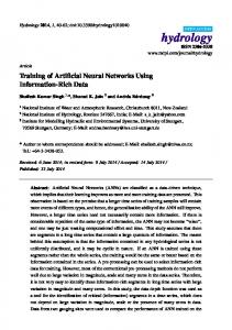
NEURAL NETWORKS A Multi Layer Perceptron Feedforward architecture (MLPFF) has been considered for the Neural Networks described in the present paper. This class of Networks, whose structure is shown in Figure 1, is generally made up by several layers: an input layer, one or more hidden layers and an output layer. Each layer contains a number of neurons that can be viewed as black – box’s with multiple inputs and multiple outputs (MIMO). The input and the output layers contain as many neurons as the number of input and output variables respectively ( X , Y in Figure 1). All the neurons are linked by means of connections upon which appropriate weights are located. _ X

input

neuron

weight

hidden

_ Y

output

Figure 1 – Scheme of a Multi layer Perceptron Feedforward Neural Network (MLPFF). 01P23-196

n

(1)

j =1

Then the output of the i-th neuron is obtained by processing the weighted sum of the inputs (1) with a transfer function (i.e. activation function), which for the current application is the non-linear bipolar sigmoid function:

h( neti ) =

1 1 + exp( −neti + bi )

(2)

where bi is a bias term. NEURAL NETWORK TRAINING A Neural Network is able to learn and generalize an input–output mapping from a set of examples which constitutes the training set. Each element of the set is a couple of vectors: the L–dimensional input vector X and the Q–dimensional output vector f(x,w). The appropriate Network weights and bias terms (see eq.’s 1 and 2) are found through a learning procedure where the following cost function is minimized by means of the Levenberg-Marquardt optimization method [17]:

E=

(

1 P Q f ( x, w) qp − y qp ∑∑ 2 P p =1 q=1

)

2

(3)

where P is the training set dimension, while y and f(x,w) are the measured and the estimated output respectively. NEURAL NETWORK GENERALIZATION As shown above the purpose of the Network training is to find the appropriate set of weights (w) and biases (b) which leads to the best fit of the learning examples. This goal is achieved by searching for the minimum of the training cost function (3). Nevertheless, this set of optimal parameters does not guarantee a satisfactory accuracy of model estimates in processing a set of independent variables not belonging to the training set. This behavior can be explained considering that if the examples are biased, the optimization method could converge to a biased solution itself, thus loosing in generalization. This risk is known as overfitting to highlight the occurrence that the Network parameters allow to reproduce accurately the selected examples, but are not optimal in the sense of minimizing the generalization error (also called true cost function) which usually assumes the same structure of eq. (3) [15], [18], [19]. In order to avoid the risk for overfitting, a cross validation procedure, coupled with a dedicated early stopping algorithm, has been followed. 2

Accordingly to this latter method, the optimization procedure is stopped at an adequate time when the Network estimation error, on a validation set, reaches a given threshold [14], [15], [17]. Moreover, the early stopping procedure avoids the occurrence of the Network overtraining by limiting the number of learning iterations on the selected examples. Hence, the improvement of model generalization is strongly influenced by the selected learning and validation data sets. Thus, the experimental data set has to be split into three parts: i) the learning, ii) the validation and iii) the test sets, which are used for the parameters optimization, the stopping criterion and the evaluation of the Network generalization, respectively. It is worth to notice that many studies have been performed in order to find the appropriate training and validation data sets. Among others, the work of Amari et al. [15] evidences the complexity of the topic. Furthermore, this task is particularly critical for the identification of the complex processes related with internal combustion engine performance, whose mapping is studied in the present work. In the following, the problem of finding the proper composition of the most informative training data set is addressed. The whole experimental data set has been randomly split into two parts: the first has been used for selecting the training examples, while the second has been adopted for both the early stopping and the model validation.

BATCH AND SEQUENTIAL ACTIVE LEARNING Two different ways of using Active Learning techniques are usually considered namely Batch and Sequential Active Learning. As shown in Figure 2 the batch approach is used when the training examples are collected by an iterative selection from an existing set of experimental data. In such case the Active Learning procedure provides the selection of the most informative data with a general reduction of the training set dimension by avoiding the inclusion of redundant information. The flow diagram of a Sequential Active Learning Procedure is shown in Figure 3. This method is used to drive the experiments by an iterative selection of the most appropriate condition to be observed (e.g. for the current application, the combination of control, operative and state engine variables). The experimental data set is then composed by the most informative data with a general reduction of dimension and a significant decrease of the experimental effort. In both Batch and Sequential Active Learning application a valuable improvement of model accuracy is achieved with a reduced number of training examples. System

Experimental data Training set

ACTIVE LEARNING In order to build-up the training set for the learning phase of a Neural Network, a number of examples is required. Each example is obtained from an experiment on the target system, by observing the system responses to a given set of inputs. The inputs can be selected accordingly to the following methodologies [11], [12], [13], [17], [20], [21], [22], [24]: i) random, ii) Heuristic, iii) Active Learning Techniques. In the former two cases the learning is called Passive since the Network behaves as a passive recipient of information. While, in case iii) the Network plays a more active role in collecting training examples by using information derived from its connection weights and biases values, which in turn give an information about the current Network state. Hence, the Active Learning allows a faster convergence with increased generalization and a lower number of examples needed for the training. Furthermore, since the training set is composed of the most informative experimental data, the model generalization is enhanced and the risk for overfitting is strongly reduced. Thus, the basic idea of Experimental Design methods is to use for the learning phase the examples whose information content guarantees an improvement of model precision.

01P23-196

Network Training

Active learning

Figure 2 – Batch Active Learning

Active Lear.

Input

System

Output

Experiment Network Training

Figure 3 – Sequential Active Learning

DATA COLLECTION In literature several approaches for the implementation of Active Learning procedures can be found, and the example selection is performed in all cases through the optimization of an appropriate mathematical functional [11], [12], [13], [20], [23]. In the paper the methods proposed by MacKay and Cohn, based on the information theory and on the minimization of the covariance estimation error respectively [11], [13], are adopted.

3

MacKay method – This method deals with the detection of the information that a new example can transfer to the Network weights during their identification. Any weight can be considered as a random variable whose variability depends on both the large spectrum of monitored independent variables (i.e. engine operating condition) and the measurement noise [19]. The information content of a new observation can be expressed as the change in the statistical entropy (also known as Shannon’s entropy) of the weights distribution [11]. In the following a training data set with dimension N+k is considered, with N initial examples and k examples selected by the Active Learning procedure. The Shannon’s entropy of the current weights distribution, whose probability density function is p(wk), can be computed through the following relationship which gives a measure of the uncertainty in the weights distribution [11], [21]:

H ( p(wk )) =

n (1 + log 2° ) + 1 log(det Vk ) 2 2

(4)

with n number of Network weights and bias terms. By considering a normal distribution for wk with mean value µk and covariance Vk, the covariance matrix Vk can be approximated as the inverse of the Hessian matrix computed for the actual estimation error E(wk)1 :

Vk = Ak−1 ≅

1 N +k ∑ g (xi )g (xi )T E (wk ) i =1

(5)

where g(xi) is the error gradient with respect to the Network weights estimated for the i-th input xi. Such gradient expresses the Network sensitivity to the input xi. When a new observation is added to the actual training set, the Network is trained with N+k+1 examples and a new optimal weights distribution p(wk+1) is detected; the updated Shannon’s entropy is then expressed by:

H ( p (wk +1 )) =

n (1 + log 2° ) + 1 log(det Vk +1 ) = 2 2 1 n = (1 + log 2° ) + log det Ak-1+1 2 2

(

)

(6)

The information transferred to the weights distribution by the new datum is estimated as [11], [21]:

I = H ( p (wk )) − H ( p (wk +1 )) =

(

)

( )

1 1 = log det Ak−1 − log det Ak−+11 2 2

(7)

Assuming that the estimation error can be quadratically approximated around wk, the covariance 1 matrix Ak−+1 can be updated by [11], [21]:

Ak−+11 = Ak−1 +

1 g (x k +1 )g (x k +1 )T E (wk )

(8)

Substituting eq. (8) in eq. (7), the information refinement due to the new observation is given by:

 1 1  g ( x k +1 ) T Ak−1 g ( x k +1 )  I = log1 + 2  E ( wk ) 

(9)

Thus, the selection of the k+1-th example of the training set is accomplished by maximizing the functional I in eq. (9), which is only dependent on the input xk+1. Moreover, since the functional I corresponds to the estimation error variance in xk+1, the new example is selected within the region where the Network estimation is inaccurate. Cohn method - The Active Learning method proposed by Cohn is based on the minimization of the generalization error in a region2 of interest. The generalization error can be analytically expressed by [13], [25]:

Eg =

1 X

∫ ( f (x, w) − y ( x ) ) dx 2

(10)

X

where X is the region of interest, f(x,w) is the estimated output for the input x and y is the corresponding observed value. The equation (10) can be approximated by [13], [21], [25]:

Eg =

1 X

  2 2  ∫ ( f ( x , w) − y ) dx + ∫ ( y − y (x )) dx  (11)  X  X

where y is the mean value of the measurements. The first term in the right hand side is the estimation error variance computed within the input region X, while the second term is a bias and is zero if the system model corresponds perfectly to the real process. The goal of the Cohn method is to minimize the generalization error, which for an unbiased process corresponds to the minimization of the error variance within the input region X. Nevertheless, the equation (11) is awkward to solve over the whole space X and the estimation error variance is computed with respect to a restricted set of examples, named reference points.

2 1

The actual estimation error corresponds to the cost function in eq. (3).

01P23-196

Note that this region of the input domain does not contain the examples belonging to the validation data set for the cross validation procedure. 4

For a reference data set with dimension M, the mean error variance has to be minimized over the M reference points:

σ 2f (x,w )

=

M

1 M

M

∑σ 2f (xi ,w )

(12)

i =1

According to the previous paragraph, some approximations can be carried out and the estimation error variance can be computed in every reference point as:

σ 2f (x i , w ) = g (xi )T A −1 g (xi )

(13)

Thus, the estimation error mean variance at the k-th iteration is given by [13], [25]:

σ 2f (x,wk )

M

(

= g T Ak−1 g + tr Ak−1C

)

(14)

where Ak−1 is the covariance matrix of weights and biases

computed

g = 1 M ∑i =1 g ( xi ) M

for

the

and

first

examples;

N+k

C = 1 M ∑i =1 g (xi )g (xi )T M

are the first and the second moments of the estimation error gradient with respect to the Network weights, evaluated in the reference points. When the training set is upgraded with a new observation, the estimation error mean variance, evaluated on the reference set (eq. 14), changes; the N+k+1-th example is then selected in order to maximize the following difference:

∆ σ 2f ( x ,w )

M

= σ 2f ( x ,wk )

M ,k

− σ 2f ( x ,wk +1 )

M ,k +1

(15)

Assuming that the error function can be quadratically approximated around wk, the equation (15) can be rewritten as [13], [25]:

∆ σ 2f ( x ,w )

M

=

g (x k +1 )Ak−1CAk−1 g (x k +1 )

E (wk ) + g (x k +1 )T Ak−1 g (x k +1 )

(16)

The relationship (16) expresses the variation of the estimation error mean variance when a new example is added to the training set. According to the Cohn method the new example is selected in order to maximize such difference, which is exclusively dependent on the input vector xk+1. In the appendix section further information on both MacKay and Cohn methods can be found. In case of batch Active Learning, a new example is selected by a direct evaluation of formulas (8) or (16) on the available examples left. This Network projection over the input domain corresponds to a direct evaluation of the functionals (8) or (16) without the recourse to a time consuming optimization algorithm. It is worth to note that for sequential Active Learning at 01P23-196

each iteration the optimization of (8) or (16) must be carried out to set the appropriate input variables (i.e. engine operating variables) corresponding to the new experiment to be performed. This latter approach results in an increase of computational time and in a more complex numerical implementation. From a mathematical point of view the problem must be recast as a constrained optimization problem with non linear constraints. The implementation of a sequential Active Learning procedure is currently underdevelopment. An off-line approach has been considered to evaluate the feasibility of the methodology, by replacing the real engine with a phenomenological model [1], [2] (i.e. white-box engine model). At the moment, one of the main problems is related with the definition of the feasible spark advance range, which in turn assumes different bounds as function of Air-Fuel ratio and engine speed. Once the off-line procedure will be assessed, the implementation of the on-line procedure will be carried out on a real system.

RESULTS The batch Active Learning methods, described in the previous paragraphs, have been implemented to train four Neural Network based black-box models to map the load torque and the HC, CO, NOx emissions of a S. I. engine. The batch Active Learning approach has been used to select the training examples from a wide set of experimental data corresponding to 469 steady state engine operating conditions. The experiments were performed at Istituto Motori – CNR in Naples on a FIAT 2.0 liters 16 valves engine, ranging the engine speed from 1000 to 3000 [rpm], the load torque from 10 to 90 [Nm], the AFR from 11 to 18 and the spark advance within the limits of an adequate combustion, avoiding the occurrence of knock or misfiring. The Neural Networks considered for the present work have one hidden layer with a different number of neurons, as it is summarized in Table I. The model inputs have been selected in order to define the engine operating conditions uniquely and are represented by the following state and control variables: engine speed, air mass per cycle, fuel mass per cycle and spark advance. It is worth to notice that the intake mass per cycle has been considered to express the engine load, rather than the manifold pressure as usually done for control oriented models. The current approach allows to simulate only the in-cylinder thermodynamic processes without accounting for intake manifold phenomena. Therefore, the resulting model is more generally applicable since it does depend neither on manifold geometry nor on intake/exhaust valve lift and/or timing. Nevertheless, the model precision could degrade because of the expected higher error in the air mass flow measurement with respect to manifold pressure [9]. All the models have been trained making use of the Active Learning methods, proposed by Cohn and 5

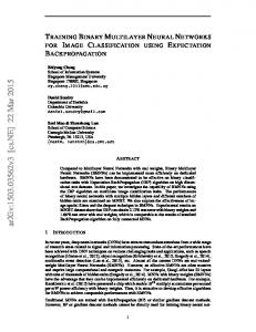
Mackay, and the passive learning approach. In case of the Active Learning methods, the training data set is initially composed of twenty points, selected close to the border of the [engine speed – load torque] experimental plane (see Figure 4). The data set is then upgraded by an iterative selection of the examples left, according to the MacKay or the Cohn algorithms. Moreover, in case of the Cohn method, the reference data set is composed by 35 points, heuristically selected as the most significant of the whole set of data. On the other hand, when the passive learning approach is adopted, the training examples selection is based on heuristic consideration. The Figure 4 shows the path followed by the MacKay method in collecting the training examples during the Active Learning of the engine torque model. The figure evidences that during the first four steps the technique selects the examples in the middle area of the plane, where a lack of information is detected.

achieved precision and the required computational effort are compatible with the application within a framework for the analysis and the optimization of automotive control strategies. The plots in Figure 5 Figure 8 and the R2 values in Table II - Table IV evidence that the Networks guarantee a good estimation even on the test data set, confirming that the Active Learning techniques allow to achieve a satisfactory model generalization. This behavior is furthermore evidenced by the results obtained making use of the passive learning method, with a heuristic selection of the training examples (see Table IV); in such case the Networks accuracy decreases strongly on the test data set with a significant decay of model generalization. 100 90

Initial data Selected data

80

In order to reduce the risk for overfitting, the early stopping method has been applied. As already mentioned, the method stops the Network training when an error threshold is reached and allows to avoid an overtraining of the selected learning examples. The models have been tested by simulating the Neural Networks on the test data set, and the estimation 2 accuracy has been expressed by means of the R index. All the information related to models performance are summarized in the Table II – Table IV, depending on the active or passive learning adopted method. The results are referred to simulations carried out on the training, the test and the global data set; this latter corresponds to the whole set of 469 experiments. In the tables the data set dimensions are also reported. Table I: Architecture of the considered Neural Networks. Model

No. of input neurons Internal (model inputs) Neurons Torque 4 - (ma,c, mc,c, rpm, SA) 15 HC 4 - (ma,c, mc,c, rpm, SA) 8 CO 4 - (ma,c, mc,c, rpm, SA) 7 NOx 4 - (ma,c, mc,c, rpm, SA) 10 ma,c = air mass per cycle; mc,c = fuel mass per cycle; rpm = engine speed; SA = spark advance.

The models estimation accuracy is graphically shown in Figure 5 - Figure 8 as comparison between predicted and observed values for the engine torque, and the HC, CO, NOx exhaust emissions. The figures illustrate the results obtained by simulating the Neural Network trained by the MacKay method, making use of both the training and test data sets. Similar results have been achieved by means of the Cohn method as it emerges in the Table II - Table IV. In all cases, the models show a satisfactory accuracy, as confirmed by 2 the R values reported in the Table II - Table IV. The 01P23-196

Torque [Nm]

70 60 50 40 30

3 2 1 4

20 10 0

1000

1500

2000 RPM

2500

3000

Figure 4 – Initial and selected training examples on the [engine speed – load torque] experimental plane. Active Learning by MacKay method. The results summarized in Table II - Table IV are plotted in Figure 9 and Figure 10. The figures show the training data set dimensions and the detected values of the correlation index R2, evidencing that for the HC and CO models the heuristic approach leads to a significant decay of model accuracy. Therefore, for HC and CO models the Active learning techniques allow to select the most informative examples, reaching a satisfactory precision (R2≅0.8) with a relatively limited training data set. On the other hand, in case of NOx models, both the active and passive learning methods guarantee a satisfactory accuracy (R2≅0.7), but with a larger set of training examples (≅300). This behavior evidences that when the Active Learning proceeds over a fixed number of examples, the relative improvement in model accuracy becomes smaller because the most informative examples are already been collected. On the other hand, in case of passive learning, an extended set of training data guarantees an increase of model accuracy. Indeed, the examples are collected heuristically and the information content of the training set statistically grows-up with its size. However, the risk for overtraining increases with the training set dimension.

6

100

60 training test

Measured NOx [g/kWh]

Measured Torque [Nm]

60

40

20

0

training test

50

80

40 30 20 10

0

20

40

60

80

100

0

0

10

Estimated Torque [Nm]

Figure 5 – Comparison between observed and estimated engine torque. Active learning by MacKay method.

20 30 40 Estimated NOx [g/kWh]

50

60

Figure 8 – Comparison between observed and estimated NOx emissions. Active learning by MacKay method.

80

Measured HC [g/kWh]

training test

Table II – Results of the Neural Networks trained by the MacKay method.

60

Active Learning – MacKay 40

Training** Ex.

R

Test Ex.

Glob* 2

R2

R

Torque 142 0.985 327 0.978 0.980

20

HC CO

0

2

0

20

40 60 Estimated HC [g/kWh]

80

NOx

103 0.930 366 0.730 0.800 80

312 0.770 157 0.750 0.740

* The global precision is estimated for the whole set of 469 data. ** The training set is initially composed of 20 examples.

Figure 6 – Comparison between observed and estimated HC emissions. Active learning by MacKay method.

Table III – Results of the Neural Networks trained by the Cohn method.

2500 training test

Active Learning – Cohn

2000 Measured CO [g/kWh]

Training** Ex.

1500

500

R2

Reference Ex.

R2

Test Ex.

R2

Glob*

R2

Torque

140

0.980 35 0.970

294 0.960 0.970

HC

237

0.780 35 0.810

197 0.760 0.790

CO

81

0.950 35 0.977

353 0.730 0.840

NOx

346

0.800 35 0.530

88

1000

0

0.900 389 0.780 0.820

0.780 0.760

* The global precision is estimated for the whole set of 469 data. ** The training set is initially composed of 20 examples.

0

500

1000 1500 Estimated CO [g/kWh]

2000

2500

Figure 7 – Comparison between observed and estimated CO emissions. Active learning by MacKay method.

01P23-196

7

Table IV – Results of the Neural Networks trained by the heuristic method. Passive Learning Training**

Test

Ex.

R2

Torque

142

0.980

327 0.930 0.950

HC

105

0.630

364 0.350 0.420

CO

89

0.910

380 0.210 0.500

NOx

289

0.710

180 0.635 0.660

Ex.

R2

Glob*

R2

* The global precision is estimated for the whole set of 469 data. ** The training set is initially composed of 20 examples.

Regarding to the engine torque model, both the active and passive learning methods lead to a satisfactory estimation accuracy. Nevertheless, the results in Figure 5 show a significant standard deviation of the models estimates around their corresponding measurements. This behavior is due to a lack of homogeneous distribution of the experimental data over the engine operating range, since the torque measurements constitute a discrete domain of five values. Thus the models are able to approximately estimate such values, but they miss accurate information in their neighborhoods. Moreover, model accuracy can be improved by training the Network either with an uniformly distributed set of available input-output data or making use of a Sequential Active Learning method. However, the accuracy of the model could be improved by processing measured data by means of data normalization, confidence analysis and outliers detection algorithms.

The results obtained with both the MacKay and Cohn algorithms have shown good model accuracy with a satisfactory level of generalization. Furthermore, a significant improvement of model precision has been achieved with respect to the recourse to a heuristic selection of training data (i.e. Passive Learning technique). These applications have confirmed the capability of Active Learning techniques in reducing the dimension of the training data set. Hence, an implementation of Active Learning techniques in sequential mode can significantly reduce the experimental effort during engine model design. In the framework of the present research, further studies are oriented to implement these techniques for the rapid prototyping of SI engine control strategies. Training Exam ples

MacKay Cohn Eurist.

400 300 200 100 0 Torque

HC

CO

NOx

Figure 9 – Number of training examples selected by the active and passive learning methods for the four considered models.

CONCLUSION

Correlation Index R2

1

In the present paper two batch Experimental Design methods have been applied for the identification of S.I. engine models based on Neural Networks. These models are oriented to predict the engine torque and the exhaust emissions (HC, CO, NOx) in the framework of a computer code for the optimal design of electronic control strategies. The study is inspired by the need to reduce the experimental effort required for the engine performance mapping together with the demand for accurate black-box engine models. Regarding to synthetic models, Experimental Design Techniques have been proven to overcome the tradeoff between high precision and limited experimental data. Two techniques based on the Active Learning approaches, originally proposed by MacKay and Cohn, have been implemented to select the most informative training examples. In the paper these methods have been described showing the potential role of such approach to improve the model generalization in accordance with the complex non linear nature of the understudied problem.

01P23-196

0.8 0.6 0.4 MacKay Cohn Heurist.

0.2 0

Torque

HC

CO

NOx

Figure 10 – Correlation index performed by the four considered models making use of the active and passive learning methods.

8

REFERENCES 1. Arsie I., Pianese C., Rizzo G., ‘Models for the Prediction of Performance and Emissions in a Spark Ignition Engine - A Sequentially Structured Approach’, SAE Paper 980779, pub. on SAE 1998 Transactions, ‘Journal of Engines’, Section 3, Vol. 106, pp. 1065-1079. 2. Arsie I., Pianese C., Rizzo G., ‘Development and Identification of a Hierarchical System of Models for Rapid Prototyping of SI Engines’, Proc. of the 6th IEEE Mediterranean Conference on "Control Systems", Alghero, Italy, June 9-11, 1998, pub. on Theory and Practice of Control and Systems 1998, World Scientific Publishing Ltd. London UK, pp. 182-188. 3. Pianese C., Rizzo G., ‘Interactive Optimization of Internal Combustion Engine Tests by means of Sequential Experiment Design’, Proc. of the 3rd Biennal Joint Conference on ‘Engineering Systems Design and Analysis – Esda 96’, Petroleum Division of ASME, Montpellier, France, July 1 – 4 1996, ASME PD Vol 80, pp. 57 – 64. 4. Arsie I., Marotta F., Pianese C., Rizzo G., ‘Identification of Spark Ignition Engine Models based on Neural Network via Experimental Design Techniques’, Proc. of the 12th IFAC SYSID 2000, Symposium on ‘System Identification’, June 21-23 2000, Santa Barbara, CA. 5. Eschenauer H., Koski J., Osyczka A., ‘Multicriteria Design Optimization’, Springler – Verlag, 1990. 6. Mowll D., Robinson D.R., Pilley A.D. (1996), Bayesian Experimental Design and its Application to Engine Research and Development, SAE Paper 961157 in SP – 1177. 7. Mowll D., Robinson D.R., Pilley A.D., Optimising Engine Performance and Emissions Using Bayesian Techniques, SAE Paper 971612 in SP – 1275. 8. Grimaldi C.N., Mariani F., On Board Diagnosis of Internal Combustion Engines: A New Model Definition and Experimental Validation, SAE Paper 970211. 9. Arsie I., Pianese C., Rizzo G., ‘Enhancement of Control Oriented Engine Models Using Neural Network’, Proc. of the 6th IEEE Mediterranean Conference on "Control Systems", Alghero, Italy, June 9-11, 1998, pub. on Theory and Practice of Control and Systems - 1998, World Scientific Publishing Ltd. London UK , pp. 465-471. 10. Arsie I., Flora R., Pianese C., Rizzo G., Serra G., Development and Validation of a Model for mechanical Efficiency in a Spark Ignition Engine, SAE Paper 1999-01-0905. 11. MacKay D.J.C., ‘Information - Based Objective Functions for Active Data Selection’, Neural Computation 4 (4), pp. 590 - 604, 1992. 12. Plutowski M., ‘Selecting Training Examples for Neural Network Learning’, PhD Thesis, University of California, San Diego, 1994.

01P23-196

13. Cohn D.A., ‘Neural Network Exploration Using Optimal Experiment Design’, AI Memo No.1491, CBCL Paper No. 99, 1994. 14. Van Gorp J., 'Nonlinear Identification With Neural Networks and Fuzzy Logic', PhD thesis, september 2000, Vrije Universiteit Brussel. 15. Amari S., Noboru M., Muller K.R., Finke M., Howard H.Y., Asymptotic Statistical Theory of Overtraining and Cross Validation, IEEE Transactions of Neural Networks, Vol. 8, No. 5, september 1997, pp. 985-996. 16. Arsie I., Flora R., Pianese C., Rizzo G., Serra G., ‘A Computer Code for S.I. Engine Control and Powertrain Simulation’, SAE Paper 2000-01-0938, on SP-1501, pp. 185-198. 17. Demuth H., Beal M., ‘Matlab Neural Network Toolbox’, The Mathworks, 1997. 18. Patterson D.W., ‘Artificial Neural Networks – Theory and Applications’, Prentice Hall, 1995. 19. Hecht – Nielsen R., ‘Neurocomputing’, Addison – Wesley, 1987. 20. Fukumizu K., ‘Dynamics of Batch Training in Multilayer Networks – The existence of Overtraining’,1998, BSIS Technical Report No.981, RIKEN Brain Science Institute, Hirosowa, Wako-shi, Saitama, JP. 21. Bard J., ‘Nonlinear Parameter Estimation’, Academic Press, 1990. 22. Fukumizu K., ‘Statistical Active Learning in Multilayer Perceptrons’, IEEE Transactions on Neural Network, Vol XX , 1999. 23. Sung K.K., Niyogi P., ‘A formulation for Active Learning with Applications to Object Detection’, AI Memo No. 1438, CBCL Paper No. 119, 1996. 24. Sahani. M., ‘Interactively Exploring A Neural code by Active Learning’, Poster in Neural Information and Coding meeting, March 16 – 19 1997. 25. Cohn D.A., ‘Active Learning with Statistical Models’, AI Memo No. 1522, CBCL Paper No. 110, 1995. 26. Lawrence S., Lee G. C., Tsoi A.C., ‘What size Neural Network gives Optimal Generalization? Convergence Properties of Back Propagation’, Technical Report UMIACS – TR – 96 – 22 e CS – TR – 3617, 1996.

CONTACT Dr. Ivan Arsie ([email protected]) Dr. Cesare Pianese ([email protected]) and Prof. Gianfranco Rizzo ([email protected]) are with the Dept. of Mechanical Engineering at University of Salerno, 84084 – Fisciano (SA), Italy. Dr. Fabrizio Marotta ([email protected]) is with the CHT dept. at Andersen Consulting - Rome, Italy. Ph. +39 089 964081, Fax +39 089 964037. http://www.dimec.unisa.it/dimec/macchine

ACKNOWLEDGEMENT The present work is funded on Italian Ministry of Research project PRIN '99 and University of Salerno project ex 60%. This research is also co-sponsored by Powertrain Control Department of Magneti Marelli. 9

DEFINITIONS, ACRONYMS, ABBREVIATIONS

1. Choice of an initial training data set.

A: Hessian matrix of the mean square error

2. Training of the Network with the current training set.

bi: Bias term for the i-th neuron 3. Check for a termination criterion. E: Mean square estimation error f(x,w): Neural Network estimation g(xi): Output sensitivity for the i-th input

4. Selection of the next input - output data or the new experimental condition on the real system. 5. Perform the experiment on the real system measurement of the output.

h(neti): Activation function for the i-th neuron H(p(w)): Shannon’s entropy for the weight w statistical distribution

6. Addition of the new couple input - output to the existing training set. 7. Go to point 2.

n: Number of Network weights and bias terms neti: Weighted sum of the inputs for the i-th neuron

For Batch Active Learning, the direct choice of the next couple input - output is performed at points 4 and 5.

p(wi):Probability density function for the i-th weight

The Mackay procedure

V: Covariance matrix of the Network weights

The procedure proposed by Mackay is based on the Shannon’s entropy concept. By assuming the randomness of experimental measures, the Network parameters (weights and biases) distribution can be described through a probability density function. Then the statistic entropy associated with this distribution is computed as follows [21]:

wij: Weight located between the i-th and the j-th neurons xk: k-th input vector X: Input domain y: Measurement

APPENDIX In the present appendix further information are given in order to improve the understanding of the procedure followed during the implementation of the methods proposed by MacKay and Cohn. It's however worth to note that, an exhaustive description of all the mathematical details is beyond the scope of the paper and the reader is addressed to the original papers of MacKay [11] and Cohn [13] [25]. In the Active Learning procedure the Network learning phase starts with a reduced data set composed of N examples (i.e. N couples of input - output experimental data). After a first training a new example is selected accordingly to the Active Learning procedure. This choice is performed with the objective of improving the current state of knowledge of the Network about the system being modeled. It is worth to notice that for the Sequential Active Learning the input data, where the next experiment has to be performed, is computed. On the other hand, for Batch Active Learning the new example is selected from the available set of input output couples. The Active Learning procedure is summarized in the following points:

01P23-196

H ( p( wk )) = − ∫ p( wk ) ⋅ log p( wk )dw

(a.1)

which increases with the variance of the parameters distribution. The relationship (a.1) expresses the Shannon's entropy after N+k training phases, performed by adding at each time a new input - output couple to the training data set. When a new example is added and the Network is trained again, the distribution of the parameters and its entropy will change. The variation of the information achieved through the addition of a new example can be related to the change in the entropy of the distribution before and after the addition of the new datum:

I = H ( p( wk )) − H ( p( wk +1 ))

(a.2)

The Active Learning procedure deals with the choice of the new input that causes an increase of the knowledge level about the system understudy. In order to make eq. (a.2) applicable, the weights (and biases) probability distribution is assumed to be Normal with mean µk and covariance matrix Vk, then the entropy (a.1) assumes the form shown in eq. (4). As reported in the main body of the text, the covariance matrix V can be expressed as the inverse of the Hessian matrix A of the mean squared error with respect to the weights (see eq. (3)). In the present application at each Active Learning step, the Hessian is taken in correspondence of the current training data set with the actual value of the weights. If wk is the vector of the 10

current weights and σ2 is the variance of the measurement distribution, A can be computed as:

1 A = 2 ∇∇E ( w) σ w = wk

(a.3)

The Ajl element of the matrix is then expressed as:

A jl =

1 ∂ 2 E ( w) σ 2 ∂w j ∂wl w = w

(a.4) k

The first and the second derivatives are computed as:

∂E 1 ∂ = ∂w j 2 ∂w j

 P   ∑ ( yi − f (xi , w ))2  =  i =1 

P

= − ∑ ( yi − f (xi , w ))⋅ i =1

(a.5)

∂f (xi , w ) ∂w j

  ∂f (xi , w ) ∂f (xi , w ) − +   P ∂w j ∂wl ∂2E  = −∑   ∂w j ∂wl ∂ 2 f (xi , w ) i =1   + ( yi − f ( xi , w) ) ∂w j ∂wl  

(a.6)

where the error function (3) has been considered for the case of one Network output (i.e. Q=1) and the training set P has dimension N+k. If the Network is an exact model of the physical system to be mapped, and the error surface has a constant curvature near w=wk, then the second term appearing at RHS in the formula (a.6) can be neglected. Under these hypotheses, the covariance matrix of the weights distribution is computed as follows:

 1 Vk = Ak-1 =  2 σ

∂f (xi , w ) ∂f (xi , w )T  ∑ ∂w  ∂w i =1  P

−1

(a.7)

=

(

)

( )

1 1 log det Ak−1 − log det Ak−+11 2 2

(a.8)

1 In order to express the covariance matrix Ak−+1 a

quadratic approximation for the mean squared error is assumed leading to:

01P23-196

1 ∂f (xk +1 , w ) ∂f (xk +1 , w ) ∂w ∂w E (wk )

T

(a.9) w = wk

By substituting eq. (a.9) and eq. (a.7) into eq. (a.8) the following expression is obtained (see eq. (9)):

1 I = log(1 + 2 +

1 ∂f (xk +1 , w)T ∂w E (wk )

Ak−1 w = wk

(a.10) ∂f (xk +1 , w) ∂w w = wk 

 1  1 = log1 + gkT (xk +1 )Ak−1 gk (xk +1 ) 2  E (wk )  Equation (a.10) depends only on the current state of the Network (i.e. the value of the actual weights wk) and on the input xk+1. The method proposed by Mackay selects the next input xk+1 as the one that gives rise to the maximum improvement in the knowledge of the physical system to be modeled. The term g kT (x k +1 )Ak−1 g k (x k +1 ) in the equation (a.10) represents the variance of the Network output in correspondence of the input xk+1. Hence, the selection of the input point xk+1, through the maximization of equation (a.10), is equivalent to choose the next experimental condition, where the measurement has to be performed, as the one that is associated with the largest model output variance. The Cohn procedure The Active Learning procedure proposed by Cohn has the aim of minimizing the generalization error of the identified model over a certain region of the input domain. This region represents the area of the working domain upon which the Neural Network must give the best performance. For the present application the region of interest could be the working domain of the engine within the ECE or the FTP test drive schedule.

w = wk

where the term σ2 is replaced by the mean squared error computed on the available training data set (see eq. (5)). By substituting eq. (4) in eq. (a.2) or (7), the information gained through the addition of a new example to the existing training data set is given by the formula (7):

I = H ( p (wk )) − H ( p (wk +1 )) =

Ak-1+ 1 = Ak-1 +

The expression for the generalization error upon the input space X is given by (see eq. (10)):

Eg =

1 X

∫ ( f (x, w ) − y (x )) dx 2

(a.11)

X

then, denoting with y the mean value of the measurements, the generalization error can be decomposed to give the relationship (11), shown in the main body of the paper. After the k-th training phase k new experimental data have been added to the initial training set. According to Cohn approach, the new input data to add to the existing training data set is the one that generates the smallest generalization error (11) over X. Under the hypothesis of a correct model structure, the second term of relationship (11) can be neglected. Then the choice of the next example to add to the training set is performed by minimizing the first 11

term which represents also the variance of the Neural Network model over the input space X. Since a direct method for computing the integral over the whole input space is not available, an approximation is taken. In order to represent the input space X, a fixed number of points, called reference points, is considered. The variance of the Network over the space X is then computed as the mean variance over the reference points. Therefore, the target is to find a new input-output couple that minimizes the mean variance over the reference points then, if the model is correct, the generalization error is reduced as well. The mean variance mentioned above after k training phases, is computed as (see eq. (12)):

σ 2f (x , wk )

M ,k

=

1 M

M

∑σ 2f (xi , wk )

(a.12)

i =1

where xi is the generic reference point, while M is the total number of the reference points and the term σ 2f (x , w ) represents the actual model variance in i

k

correspondence of the i-th reference point. Each term of the sum can be computed as:

σ 2f (xi , wk ) = gkT (xi )Ak−1 gk (xi )

(a.13)

Through relationship (a.13) the mean variance over the reference points (a.12) can be rewritten as:

σ 2f (xi , wk )

M ,k

(

= g Tk Ak−1 g k + tr Ak−1C k

)

(a.14)

where the first and the second moments of the estimation error gradient with respect to the Network parameters are evaluated making use of the following relationships:

gk = Ck =

1 M 1 M

M

∑ gk (xi ) i =1

reference points will change in σ 2f (x ,w ) i k +1

M ,k +1

. Thus,

the overall variation will be given by the following relationship:

∆ σ 2f (x , w )

M

= σ 2f (x , wk )

M ,k

− σ 2f (x , wk +1 )

M , k +1

(a.16)

The new model variance over a single reference point can be computed as:

σ 2f (xi , wk +1 ) = g k (xi )T Ak−+11 g k (xi )

(a.17)

then by using relationship (a.9) the variance in a single reference point (a.17) is:

[

σ 2f (xi , wk +1 ) = g k (xi )T Ak−1 − +

Ak−1 g k (xk +1 )gk (xk +1 ) Ak−1   g k (xi ) T E (wk ) + g k (xi ) Ak−1 gk (xi ) T

= g k (xi )T Ak−1 g k (xi ) −

(

(a.18)

)

2 T   g k (xi ) Ak−1 g k (xi )   + T  E (wk ) + g k (xk +1 ) Ak−1 g k (xk +1 )

By taking the mean value of (a.18) over the reference points and substituting it in equation (a.16), the change in the mean variance value over the reference points is:

∆ σ 2f (x , w )

M

=

gk (xk +1 )T Ak−1CAk−1 gk (xk +1 ) (a.19) E (wk ) + gk (xk +1 )T Ak−1 gk (xk +1 )

Hence, minimizing the new variance value over the reference points is equivalent to maximize the functional (a.18), which depends only upon the current state of the Network. Finally, the consideration made at the end of the previous section for the MacKay case can be extended for the Cohn method as well.

(a.15)

M

∑ gk (xi )gk (xi )T i =1

When a new example is added to the training set and the Network is trained, the mean variance over the

01P23-196

12