Integer-Valued, Minimax Robust Designs for Estimation ... - CiteSeerX

Integer-Valued, Minimax Robust Designs for Estimation and Extrapolation in Heteroscedastic, Approximately Linear Models Zhide Fang; Douglas P. Wiens Journal of the American Statistical Association, Vol. 95, No. 451. (Sep., 2000), pp. 807-818. Stable URL: http://links.jstor.org/sici?sici=0162-1459%28200009%2995%3A451%3C807%3AIMRDFE%3E2.0.CO%3B2-D Journal of the American Statistical Association is currently published by American Statistical Association.

Your use of the JSTOR archive indicates your acceptance of JSTOR's Terms and Conditions of Use, available at http://www.jstor.org/about/terms.html. JSTOR's Terms and Conditions of Use provides, in part, that unless you have obtained prior permission, you may not download an entire issue of a journal or multiple copies of articles, and you may use content in the JSTOR archive only for your personal, non-commercial use. Please contact the publisher regarding any further use of this work. Publisher contact information may be obtained at http://www.jstor.org/journals/astata.html. Each copy of any part of a JSTOR transmission must contain the same copyright notice that appears on the screen or printed page of such transmission.

JSTOR is an independent not-for-profit organization dedicated to and preserving a digital archive of scholarly journals. For more information regarding JSTOR, please contact [email protected].

http://www.jstor.org Sat Mar 31 14:28:34 2007

Integer-Valued, Minimax Robust Designs for Estimation and Extrapolation in Heteroscedastic, Approximately Linear Models Zhide FANGand Douglas P. WIENS

We present our findings on a new approach to robust regression design. This approach differs from previous investigations into this area in three respects: the use of a finite design space, the use of simulated annealing to carry out the numerical minimization problems, and in our search for integer-valued, rather than continuous, designs. We present designs for the situation in which the response is thought to be approximately polynomial. We also discuss the cases of approximate first- and second-order multiple regression. In each case we allow for possible heteroscedasticity and also obtain minimax regression weights. The results are extended to cover extrapolation of the regression response to regions outside of the design space. A case study involving doseresponse experimentation is undertaken. The optimal robust designs, which protect against bias as well as variance, can be roughly described as being obtained from the classical variance-minimizing designs by replacing replicates with clusters of observations at nearby but distinct sites. KEY WORDS: Bioassay; Carcinogen; Dose response; Efficient rounding; Finite design space; Fisher consistency; Logistic model; Polynomial regression; Probit model; Quota rounding; Second-order design; Simulated annealing; Weighted least squares.

1.

INTRODUCTION

In this article we present our findings on a new approach to robust regression design. As was done by Box and Draper (1959), Li and Notz (1982), Marcus and Sacks (1976), Pesotchinsky (1982), and Wiens (1992, 1998), to name but a few contributors, we seek robustness against departures from the assumed linear response function and/or from the assumption of homoscedasticity. Our model allows for such departures of a very general form. One way in which this work differs from that of the aforementioned authors is in our use of a finite design space. To our knowledge, robust regression designs under this restriction have previously been investigated only by Li (1984). The number of possible design points may be arbitrarily large, so that finiteness is not a practical restriction. The mathematical problem is, however, reduced to a finitedimensional one, resulting in a considerable simplification both analytically and numerically. The formulation of the problem of Li (1984) led to a linear programming problem sufficiently involved as to limit the investigation to the case of straight line regression over an interval. In contrast, we use an easily implemented simulated annealing algorithm that yields (near-) optimal solutions with no restrictions on the fitted model or on the structure of the design space. A general discussion of simulated annealing algorithms, with an application to a nonlinear design problem, has been given by Bohachevsky, Johnson, and Stein (1986). Haines (1987) and Meyer and NachtZhide Fang is Visiting Professor, Department of Mathematics, University of New Orleans, Lakefront, New Orleans, LA 70148 (E-mail: ~u~zg@mntlz.~tno.edlr). Douglas Wiens is Professor of Statistics, Department of Mathematical Sciences, University of Alberta, Edmonton, Alberta, Canada T6G 2G1 (E-mail: doug.~viens@zialbei'tn.cu).This research is supported by the Natural Sciences and Engineering Research Council of Canada. The authors acknowledge the helpful comments of the editor, an associate editor, and a referee in the preparation of this article.

sheim (1988) took this approach in constructing optimal designs assuming the fitted (linear, homoscedastic) model to be exactly correct. The final departure from previous work lies in our search for integer-valued, rather than continuous, designs. Previous approaches have generally resulted in "designs" that are arbitrary and possibly continuous probability functions [(x) on the design space. The number of observations allocated to a particular design point x, is then n[(x,),with the experimenter left to approximate this quantity when, as is typically the case, it is not an integer. In two of the three classes of problems considered here, the annealing algorithm gives exact integer-valued designs; that is, n[(x,)is an integer. In the remaining case, although the designs need not be exact, we use and compare two methods of obtaining integer-valued approximations to n[(x,). We begin with a discussion of our model of approximate linearity and possible heteroscedasticity. We follow with a description of the design problems for which we seek solutions. In Section 2 we reduce these problems to numerical minimization problems. In Sections 3-5 we give the annealing algorithms, and examples of the minimum loss designs, for polynomial regression over an interval and for first- or second-order multiple regression over a multidimensional cube. In Section 6 we extend our results to the case of extrapolation, and apply them to a case study involving dose-response experimentation. In Section 7 we give conclusions and guidelines based on the observation that the optimal robust designs, which protect against bias and heteroscedasticity, can be roughly described as being obtained from the classical, (homogeneous) variance-minimizing designs by replacing replicates by clusters of observations at nearby but distinct sites. @ 2000 American Statistical Association Journal of the American Statistical Association September 2000, Vol. 95, No. 451, Theory and Methods

808

1.1

Journal of the American Statistical Association, September 2000

Statistical Model

The statistical model under consideration is initially formulated simply as a general regression model with additive errors, Y = E[Ylx]+ E . Possible design points x, ( i = I,. . . , N) are specified in advance and generally will be equally spaced over the region to be explored by the experimenter. At these points, uncorrelated observations Xj may be taken. The experimenter is to allocate n, > 0 obni = n specified in advance. servations to x,, with The design problem is to choose nl: . . . , n ~ in an optimal manner. The mean response E[Yjx]is thought to be well approximated by a linear combination zT(x)f3of p regressors ( z l ( x ) :. . . , z , ( ~ ) )=~ z ( x ) . We assume throughout this article that the number of distinct locations at which ni > 0 exceeds p. As is common in robustness problems in which the population being sampled may be incorrectly specified, one must decide beforehand exactly what is being estimated. Somewhat akin to the imposition of Fisher consistency in robust estimation problems, we define the parameter vector so as to minimize the average squared error of the approximation E[Ylx]= zT(x)f3,

Write f ( x ) = E[Ylx]- zT(x)O,so that the model becomes

This corresponds to the classical notion of I-optimality ("integrated variance"), termed Q-optimality by Fedorov (1972), with respect to which Studden (1977) characterized designs for exact polynomial regression. Huber (1975) used this loss function to obtain continuous robust designs for approximate straight line regression; Wiens (1990) extended Huber's theory to the case of multiple, approximately linear regression. 1.2

Design Problems

By a design, we mean a probability distribution { p , ) f l l on the design space S = {x,)$Ll;if p, = n,/n for integers n, > 0,then we say that the design is integer valued. Such a design is implemented by assigning n, observations to x,. We consider the following problems: PI. Take B = ( 1 ) .W = ( 1 ) and find an integer-valued design that minimizes the maximum, over f , value of the loss. Such a design is to be used with ordinary least squares estimation when the errors are assumed to be homoscedastic. P2. Take W = ( 1 ) and find an integer-valued design that minimizes the maximum over f and g, value of the loss. Such a design is to be used with OLS estimation when the errors may be heteroscedastic. P3. Find an integer-valued design and weights that minimize the maximum, over f and g , value of the loss. Such a design is to be used with weighted least squares (WLS) estimation when the errors may be heteroscedastic. It turns out that we must be content with an approximate solution to this problem. 2.

where, by virtue of (I),

To bound the bias of an estimate 0, we also assume that

PRELIMINARIES

Let { p i = niln):, be an integer-valued design on S. Without loss of generality, we assume the weights to be normed in such a way that = 1 and define m, = p,wi; then { m , ) ~ ?is, a probability distribution on S satisfying

-

for a given constant 172. For OLS, mi p,. We allow for possibly heteroscedastic errors, var[&(xi)] = Let Z be the N xp matrix with rows z T ( x l ).,. . , z T ( x N ) , g2g,, where g, = g(x,)for g E B satisfying and define f = ( , f ( x l ) :. .. : f ( x . ~ ) Let ) ~ .G: W , and M be iV x AT diagonal matrices with diagonal elements { g i ) , {w,}, and {mi). Assume that Z is of full rank p and let Z = U I V x p A p x pbe V the ~ psingular value decomposition, with UTU = V T V = I , and A diagonal and invertible. AugThe special case B = ( 1 ) corresponds to homoscedastic ment u by f i N x l V - , in such a way that [ u ~ U ] , \ ~ , N is orerrors. thogonal. Then by (3) and (4), we have that there is an The estimation method is least squares, possibly weighted i V - p x 1 vector c, with ilcil < 1, satisfying with weights w, = w(x,) for w E W. The special case W = ( 1 ) corresponds to ordinary least squares (OLS). As a loss function, we take the average mean squared error (AMSE) I of ~ ( x= )zT(x)8as an estimate of E [ Y x ] , Finally, define p x p matrices M j = U T M JU for j = 1 , 2 and

Fang and Wiens: Integer-Valued Robust Designs

809

In this notation, the WLS estimate

has bias vector d cov[8] given by

:=

E[B

-

81 and covariance matrix C :=

and C

=

o2

nawiz(xa)zT(xi)

n,w:giz(xi)zT ( x i )

i=l

n:wz(x;)z~(x:) i=l

=

Lemma 1. The maximum, over vectors c with ilcli < 1, of I + is the largest eigenvalue A, of M ; l M 2 M ; l . The maximizing c is the unit eigenvector of ~ J ~ M U M ; ~ Ubelonging ~ M U to its maximum eigenvalue Am - 1. From Lemma 1 and (12), we immediately obtain Theorem 1.

fJT~~~,2~T~c

(5

x

over f and g, loss and to then minimize this maximum loss l . minimizations can equivover { w i ) K 1 and { p , ) ~ ~The alently be done over { w , ) ~ and ~ , { m , ) ~ subject , to (7). The maximizations over f and g , and the minimization over { w , ) ~ ~can , , then be evaluated algebraically. This leaves only one numerical minimization over {m,)fLl. Fix a design mi}^, on S. Lemma 1, which is required for the maximization of (12) over f , follows from the ob. ; ~ servation that the nonzero eigenvalues of ~ J ~ M U M M ; ~ u ~ M are U the same as those of

Theorem 1. For OLS estimation with homoscedastic errors, (G = { I ) ,W = ( 1 ) ) we have

o2 (Z~MZ)-~Z~MWGZ(Z~MZ)-~ n

-

Our results depend on r12 and o 2 only through u := 0 2 / ( n i 1 2 which ), can be chosen by the experimenter to re- and SO the minimax design for PI has { p , ) t ~ = l mi)^^,, where {ma}El minimizes (13). For computational Purflect his view of the relative importance of variance verm,li = tr M?. The least favorPo"Sl we note that sus bias. From (6), using (2), (lo), (1 l), and finally (8), the able response contaminant f is determined by (8), where c AMSE I = I ( % g: , w , m ) is is as in Lemma 1. N To obtain the maximum loss under heteroscedasticity, we 1 I ( f , g , w . m )= xi)] - z ~ ( x , ) ~ ) ~ must maximize (12) over g; this is a straightforward appliAT %=I cation of the Cauchy-Schwarz inequality.

zLl

. 1

+ =

=

1

1

1

dTzTzd N 1 - f T ~ N

f i12

N

1

var [ ~ ( x , + ) ]g 1f 2 ( x i ) ,=I ~=l

-

o + n\

=

N

N

+

Lemma 2.

,-4

ject to ( 5 ) is attained with gi rn m2wili. Lemma 2, tbgether with Lemma 1 and (12), give

1 - tr ( Z C Z ~ ) - f T f N N

1

The maximum value of C ;N= , miwigil, sub-

+

rnaxI(.f,g,w,m)

~

~

;

2

+I

CmZw,gzli N i=l

~

T

~

f

f,s

= i12 fTf

Designs Solving Problems P I , P2, and P3

Problems PI-P3 require us to evaluate the maximum,

+

n

w

1

'

2

} , (14)

from which Theorem 2 is immediate.

+ ~ J ~ M U M ; ~ U ~ M U ) CTheorem 2.

tCT(1

{ A

For OLS estimation ( W eroscedastic errors, we have

=

( 1 ) ) with het-

Journal of the American Statistical Association, September 2000

810

and so the minimax design for P2 has {p,),N=l= { m i } g l , where {m,}:?, minimizes (15). The maximum loss (14) for WLS can be minimized over the weights with the aid of a Lagrange multiplier. The result of this minimization is given by Lemma 3.

xZl

Lerrlmn 3. The minimum value of ( n ~ , , w ~ lsub,)~ ject to (7) is m,4131,2'3)3, attained with wi cx m,-1/3172/3 , whenever mi > 0. Lemmas 1, 2, and 3, together with (12), now give Theorem 3.

(EL,

Theorem 3. For WLS estimation with heteroscedastic errors. we have

4/3 2/3

The minimax design { p i ) ~ for ~ l P3 has pi oc mi li , where {mi):=l minimizes (16). The least favorable variances satisfy g, cx fi and the optimum weights satisfy wi oc m i l p i whenever mi > 0. The motivation for considering P3 is that, as seen in (12), the loss has two distinct components. One-the bias component-arises purely from the effect of f . The otherthe variance component-arises purely from the effect of g. It thus seems plausible that one could reduce one component through an appropriate choice of design points, and the other through a judicious choice of weights. This is what we attempt to do through the minimization of (16); see Section 4.3 for a numerical indication that the venture can be quite successful. An interesting special case of Theorem 3 is v = 0 , in which case the design and weights minimize the maximum bias measure ,A - 1. We can in any event impose unbiasedness by requiring that mi = N - l , resulting in the absolute minimum A, = 1. In this case the li are proportional to the diagonal elements hii of the hat matrix H = z ( z T z ) - l z T , and we have Corollary 1.

Corollary 1. The design with pi oc h:/3 and wi cx minimizes the maximum AMSE, subject to the side condition that ~ [ 0=]0 for all f . 3. 3.1

EXACT DESIGNS FOR P I AND P2; POLYNOMIAL RESPONSE

Description of the Simulated Annealing Algorithm

We consider approximate polynomial regression; that is, z ( x ) = ( 1 . 2 , z 2 . . . . , Z P - ~ )on ~ ,[ - I . I ] . For simplicity, we assume that one of (n.itT)is a multiple of the other. If n < itT,then we also require that they have the same parity. We take equally spaced design points,

A simulated annealing algorithm, in general, consists of the following: 1. A description of the initial state of the process; that is, of the starting vector of allocations n = ( n l ,. . . : nlv) 2. A scheme by which subsequent states are generated 3. A criterion according to which these subsequent states are accepted or rejected. If n > itT,then the initial state is the uniform design, with n, = n/itTfor i = 1, . . . . N . If n 5 N , then this vector of frequencies assigned to X I , . . . , xly starts with the vector formed by repeating the vector ( 1 , 0 , . . . , 0 ) (with N / n - 1 0's) [ n / 2 ]times. This is followed by the same vector with the order of its elements reversed. If N is odd, then also a vector ( 0 , . . . , O . 1 , 0 , . . . , 0 ) of length N / n is inserted in the middle. Thus in either case the initial design is symmetric and at least close to uniform. We impose symmetry on the designs largely for its intuitive appeal. However, we remark that searches for better, possibly asymmetric, designs have yielded no improvements. To generate new designs, first define v to be the [ N / 2 ]x 1 vector consisting of the initial segment ( n l , . . . . n [ , ~ / 2 of 1) the current allocation vector. Define

with cardinalities j+ 2 1 and jo. Generate a Bernoulli random variable,

A with probability &.

1, with probability

B=

\ 0,

If j+ 2 2, then choose two indices ( t l , t 2 )from J+, at random and without replacement, and (if B = 1) pick an index to from Jo, at random. Replace v by the vector G whose elements are those of v except for

Eta

= zto

Et2

=

+B ,

zt2 + 1 - B .

Etl

= ztl

-

1,

and

(18)

If j+ = 1, then pick t o from .Jo at random, let tl be the element of J+, and replace (18) by

If N is even, then let ii = (111,. . . , f i N ) = ( E l , .. . , El\rIZ, 6 N / 2 ,. . . . El), thus preserving symmetry. If N is odd, then a further Bernoulli experiment is simulated, with probability l / N of "success." If a success is obtained, then, with 1 frequency assigned to 0) is probability 112, ~ ~ [ ~ \ r / 2 1 +(the increased by 2, with these taken randomly and symmetrically from the remaining n,. With the remaining probability 112, n [ N / 2 ~is+reduced l by 2, with these allocated randomly and symmetrically to the remaining n,. If n[N/2j+1 < 2, then this step is omitted. Then ii is constructed as earlier, with also the inclusion of the new frequency 11[l\r/21+1. To accept or reject ii as the next state, first evaluate the loss I = I ( i i ) . If I ( i i ) < I ( n ) , then ii is accepted and iterations continue. If A I = I ( i i ) - I ( n ) > 0 , then ii is accepted with probability e x p ( - N I T ) , where T is a user-chosen parameter. Following Haines (1987), we initially choose T

Fang and Wiens: Integer-Valued Robust Designs

in such a way that the acceptance rate is at least 50%; this parameter is then progressively decreased. As discussed by Press, Flannery, Teukolsky, and Vetterling (1989), we decrease T by a factor of .9 after each 100 iterations. The timing parameters were decided on partly by trial and error. Decreasing T too quickly-in particular, implementing a pure descent algorithm by setting T = 0-often caused the process to become trapped in a local minimum. We satisfied ourselves that the final minimum was global by running the algorithm several times, with a variety of timing parameters. All computations were carried out using S-PLUS; the relevant code is available from the authors on request. 3.2

Examples

81 1

change only slowly with changes in u.Figure 1 displays case PI; Figure 2 displays case P2. A message illustrated in these figures, and obtained by us quite generally, is that in the presence of bias and heteroscedasticity, making new observations at nearby sites seems to be preferable to replication at the same site. These sites are located close to those at which replicates would be taken if bias and heteroscedasticity were ignored and homogeneous variance alone were minimized. The end result is sometimes a near-uniformity, which then also supports the remark of Box and Draper (1959, p. 622) that "the optimal design in typical situations in which both variance and bias occur is very nearly the same as would be obtained if variance were ignored completely and the experiment designed so as to minimize bias alone." We have quantified the cost, in terms of lost efficiency, of the robustness given by these designs. Our measure of this efficiency is the ratio of the variance component [= N - 1 C!Y m,g,l, in (12)] of the loss when the design is constructed assuming the fitted response to be correct (f (.) = 0), to this term for the minimax design. For P I , this resulted in an efficiency of 96.7%. We first compared the minimax design for P2 to the design derived assuming both f (.) = 0 and homoscedastic errors, and with both designs evaluated under these assumptions; this gave an efficiency of 90.0%. When we compared this minimax design to the design derived assuming f (.) = 0 but heteroscedastic errors, and with both designs then evaluated at their least favorable variance functions, the resulting efficiency was 99.7%. It thus appears that the robustness is obtained quite inexpensively.

We first discuss some limiting cases, where it is possible to compare our results with the known solutions to closely related problems. If v = 0,so that only bias is a consideration, then by (3) and (9), the best continuous design has p, N - 1 . , that is, is uniform on {z,):,. With our restriction to integer-valued designs, exact uniformity is not attainable unless n is a multiple of N , and in such cases our annealing algorithm converges to the uniform design. Otherwise, the final designs are approximately uniform, with the approximations serving to bring the total number of observations up to n. As u + m, one anticipates that the designs should approach their classically optimal counterparts that minimize variance alone. We have considered in particular the case of approximate cubic regression ( p = 4) with n = 20 and N = 40. With a finite design space, there is no previous theory that applies. But because our equally spaced design 4. APPROXIMATE DESIGNS FOR P3; points (17) discretize the interval [-I, 11,Studden's (1977) POLYNOMIAL RESPONSE results for continuous I-optimal designs over this interval For problem P3, the transition from the probabilities may be taken as a guide. Studden found that the I-optimal { m i ) ~to~ the l probabilities {p,):, makes it very diffidesign places mass .I545 and .3455 at *I and *.447. Our cult to obtain exact integer-valued designs. One could of algorithm results in a design placing 3 of the 20 observacourse apply the methods of the previous section to obtain tions at each of *l and 7 at each of *.436 if the errors mi with the nmi being integers, but there is probabilities are homoscedastic (problem Pl). The points *.436 are the no guarantee that this property would be retained by the nearest, in our design space, to *.447, so that our algorithm pi. We thus obtain designs without the integer restriction, attains the closest approximation to Studden's solution. For heteroscedastic errors (problem P2), our design is very sim- then discuss ways in which these can be approximated by ilar to that in Figure 2(b), the only difference being that the integer-valued designs. sites *.231 are moved to *.538. Figures 1 and 2 illustrate examples of designs obtained 4.1 Description of the Simulated Annealing Algorithm using u = 10 and 172 = 1. We have found that the designs We describe the algorithm for AT even; in the odd case,

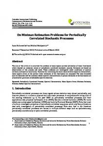
Figure 1. Exact Integer-Valued Design for Approximate Cubic Regression and Case PI With n = 20, N = 40, and u = 10. (a) Loss I(n) versus iteration number. Vertical bars above horizontal axis indicate occurrences of minimax design, with loss I = 34.28. (b) Design points and frequencies.

Journal of the American Statistical Association, September 2000

Figure 2. Exact Integer-Valued Design for Approximate Cubic Regression and Case P2 with n = 20, N = 40, and u = 10. The setup is the same as for Figure 1. Minimax loss is I = 51.41.

an adjustment analogous to that in the previous section is made. We take the same initial state as in Section 3.1, define v to be the N/2 x 1 vector consisting of the initial segment ( m l .. . . . m N I 2 o) f the current vector m of probabilities, and define J+. Jo, and B as before. The next possible state is generated as follows. If B = 1 or if j+ = .1, then we pick indices t o E Jo and tl E J+ at random and proceed as in Section 3.1, but replace (18) by

If B = 0, then we pick indices tl and t2 E J+, and replace (19) by

where U is a random variable uniformly distributed over [O, 11. For all other indices, put v, = 6,. Because these fii may now not be probabilities, we next replace them by 7)(6,)/(2 7 ) ( V i ) ) for i = 1 : . . . , N/2, where $ ( v ) = inin(inax(v,O), . 5 ) . The {fii),"=/? so obtained are then in [O, .5] and sum to .5. Finally, let rG = (ml,. . . , m,) = ( G l : . . . , 'UlVl2, V N l 2 : . . . , G I ) . The criterion for acceptance or rejection of this and subsequent states is as in Section 3.1.

c::':

4.2

Approximation Methods

Once the minimizing probabilities { m , ) ~ are ~ , determined by annealing, the probabilities pi)^, are determined as in Theorem 3. The problem is now to approximate the allocations ni = np, by integers ni in a suitable fashion. We have implemented and compared two approximation methods: 1. The minimum norm method (termed the quota method in Pukelsheim 1993), as used by Kiefer (1971). This minimizes the I , norm between the {n,) and the {fii),for any p. It is implemented by first rounding down the ni to their integer parts [nil,and then distributing the discrepancy n - C [ n i ]among those xi for which the fractional parts ni - [nil are the greatest. If the discrepancy is odd, then one more observation is allocated to 0 before this process is carried out. 2. The multiplier; or efficient rounding, method proposed by Pukelsheim and Rieder (1992). In this method, slightly modified here to preserve symmetry, one first computes frequencies fii = [ ( n- .51)p,l, where r.1 denotes rounding up

to the next integer and 1 is the number of n, > 0. Then one loops until the discrepancy n - C 6, is 0, either increasing a frequency ii, that attains 6,/n, = minnt,o 6,/n, to K, + 1 or decreasing an ii, that attains (ii, - l ) / n , = max,z,o(fi, - l ) / n , to f i , - 1. As in the minimum norm method, if the discrepancy is odd, then a preliminary adis justment is made before the looping begins: iirN121-1 decreased by 1 if it is positive, and increased by 1 otherwise. The looping is then applied only to the remaining frequencies. These increases and decreases are made sequentially and hence are not uniquely determined. In our implementation we have first increased those for which the support points are largest in absolute value, and first decreased those for which the support points are smallest in absolute value. The net effect is to move relatively more mass toward the extremes of the design space. After obtaining the integer allocations n, by one of these methods, we compute weights w, as in Lemma 3, and then compute the loss by evaluating (14) at wi and mi = niwi/n. Lest the reader think that we have missed something obvious, we remark that we investigated the option of computing both integer-valued approximations after each iteration of the annealing algorithm and basing the choice of the next state on the minimum of the two losses associated with these integer designs. This approach typically gave quick convergence to a design with loss about one unit greater than that of the optimum, but then gave no further progress. The reason appears to be that due to the rounding, small changes in the { m i }very often resulted in the same values {n,).There was then no change in the loss and no reason to change states. Our numerical studies have indicated that the two approximation methods often yield identical or almost identical results. Of course the designer can, and probably should, compute selections of both methods in each application. We have also noticed that the losses of the integer-valued designs can be lower when nonoptimal allocations npi are being approximated. Indeed, this is implied by the fact that the approximate solution to P2 in Figure 3 does not coincide with the exact integer-valued solution in Figure 2. 4.3

Examples

The methods of this section can be applied to problems P1 and P2 as well, thus affording a means of assessing the quality of the approximation methods. For the model and

Fang and Wiens: Integer-Valued Robust Designs

parameters of Section 3.2, both approximation methods resulted in the same design for P1 as there, illustrated in Figure 1. The loss associated with this design is very close34.28 versus 34.03-to that of the non-integer-valued design being approximated. For P2, both approximation methods again resulted in the same design, whose loss is about 3% greater than that of the exact integer-valued design. This loss for the exact design in turn exceeds that of the noninteger-valued design by about 3%. We have obtained weights and designs for approximate cubic regression and problem P3, using the same parameters as were used in Section 3.2 (see Fig. 3(b)-(d)). In this case the multiplier method resulted in a slightly higher loss than the minimum norm method. Plots (not shown) of the least favorable f reveal that for all three problems, m, is roughly proportional to 1 f i l . In P2 we find that gi is increasing in / x i /within each cluster of design points. In P3, however, gi is decreasing in / x i / In this latter case are we within each such cluster, as is wi. then designing for a particularly unlikely contingency, at the cost of protection against more realistic departures from homoscedasticity? To give a partial answer to this question, we assessed the performance of our designs assuming that the true variance function was known to be of the form g,* cx 1+c/xi 1" normed to satisfy ( 5 ) with equality. We computed the maximum (over f ) loss of the exact designs for P1 and P2 and the two approximate designs-both with the minimax weights and with optimal weights w? cx l/g$-for P3. These maxima are displayed in Table 1. Note that with the minimum norm approximation, the minimax weights

813

in fact result in a smaller loss than do the optimal weights. This is presumably due to the bias reduction effected by the minimax weights, as anticipated in the discussion following Theorem 3. 5. DESIGNS FOR FIRST- AND SECOND-ORDER MULTIPLE REGRESSION

In this section we outline a method by which the theoretical and computational methods of the preceding sections can be adapted to the q-variate approximate regression model, and discuss the qualitative features of the resulting designs. For these models, x = ( z l , . . . , z , ) ~and z(x) has elements 1,x l , . . . . x, and possibly second order terms xix3 (1 5 i < j < q). Thus p = q + 1 for first-order models, and p = (q l ) ( q 2)/2 for second-order models. As design space, we take the q-fold Cartesian product S = S1 x . . . x S,,where each Sj consists of ATo equally spaced points in [-I, I], as at (17) with N replaced by ATo. Thus AT = N:. There being no a priori reason to prefer one axis to another, we require that the designs be exchangeable and symmetric in each variable. Such designs can be generated by symmetrically choosing no points on the XIaxis and then forming the q-fold Cartesian product of these points with themselves, whence n = n:. We assume that no and Noare restricted in the same way as were n and N in Sections 3 and 4. The algorithms of those sections may then be used to choose the ,no points, so that the computational complexity does not increase with the dimensionality. Our simulations with q = 2 have led to the following observations. Recall that the classical designs that mini-

+

+

Figure 3. Integer-Valued Approximations, Using the Annealing Scheme and Approximation Methods of Section 4, to the Minimax Designs; n = 20, N = 40, and v = 10. For P I , both approximations result in the exact design of Figure 1. (a) P2, both approximations, loss I = 52.58. (b) P3, regression weights. (c) P3, minimum norm approximation, loss I = 52.03. (d) P3, multiplier approximation, loss I = 52.99. The losses associated with the non-integer-valued designs being approximated are P I , I = 34.03; P2, I = 49.83; and P3, I = 49.20.

Journal of the American Statistical Association, September 2000

814 Table I . Losses Associated With Variance Functions g; x 1 + c xi Under Various Design and Weight Combinations P3, minimum norm

c

d

PI

P2

Minimax weights

Optimal weights

P3, multiplier

Minimax weights

Optimal weights

mize variance alone are formed, in the Cartesian manner described earlier, from sites at xl = &I for the first-order model, and as well zl = 0 for the second-order model. The robust designs for the second-order model move mass away from the corners of the design space and into more central sites. They also do this, but to a lesser extent, for the first-order model. Furthermore, relative to the varianceminimizing designs, the robust designs replace replicates with clusters. For instance, if no = 7, we find that the robust = 21 are (for each of P I , P2, first-order designs with and P3) given by the Cartesian product of ( 0 , * . 8 . 1 . 9 , * I ) with itself. Thus there are clusters of nine points in each corner, with as well three points near the middle of each axis and one center point. The second-order designs are instead formed from ( 0 , * . I , 1 . 9 . i l ) , with four points clustered in each corner, six points in the middle of each axis, and nine points near the center. The solution for P3 gives very little weight to the center point of the first-order design, and weights all other points approximately equally in the other cases. We also note that the rounding mechanisms used for P3 can sometimes slightly alter the Cartesian product property. Calculations such as those described at the end of Section 3 gave efficiencies of 90.6%, 90.6%, and 100% for the first-order designs, and 93.3%, 93.3%, and 100% for the second-order designs. The robust designs thus seem very sensible. Their emphasis on near, rather than exact, replication protects against model bias and allows for the estimation of alternate models; the clustering makes them fairly efficient when the fitted model is in fact correct. 6.

of a certain order but to be otherwise arbitrary, to one point outside of the design interval. These results were corrected and extended by Huang and Studden (1988). Draper and Herzberg (1973) extended the methods of Box and Draper (1959) to extrapolation under response uncertainty. In their approach, one estimates a first-order model but designs with the possibility of a second-order model in mind; the goal is extrapolation to one fixed point outside of the spherical design space. In earlier work (Fang and Wiens 1999), we obtained approximate (i.e., continuous) designs robust against departures from linearity and homoscedasticity similar to those entertained in this article. The goal there was extrapolation to a region of positive Lebesgue measure. Our model is as described by (1)-(5) for x E S . For x E 7,it is given by Y = z T ( x ) B + f T ( x ) + E , where the function fT is constrained only by its L 2 ( p ) norm,

for some measure p and a given constant rl;. Important special cases are T , an interval; p, Lebesgue measure; and 7,a point at which p places unit mass. As a loss function, we take the maximum, over all f ~ satisfying (20), value of the integrated mean squared prediction error (IMSPE),

Define a p x p matrix, AT = ST z ( x ) z T ( x ) p ( d x ) ,of rank be a p x q square root of AT and define q I p. Let Q,,, = A - ~ v T A $ / ~ . Let

and define r T , = ~ rlT/(m17). Using this notation, we first calculate that

EXTRAPOLATION DESIGNS

In this section we consider designs for the extrapolation of the estimates of the mean response, determined from observations made within the design space S , to an extrapolation region 7 disjoint from S . Extrapolation is an inherently risky procedure, exacerbated by an overreliance on model assumptions; for this reason, robustness against model violations is particularly important in such applications. Designs for extrapolation of polynomials, assuming a correctly specified response, were studied by Hoe1 and Levine (1964) and Kiefer and Wolfowitz (1964a,b). Studden (1971) studied such problems for multivariate polynomial models. Dette and Wong (1996) and Spruill (1984) constructed extrapolation designs for polynomial regression, robust against various misspecifications of the degree of the polynomial. Huber (1975) obtained designs for extrapolation of a response, assumed to have a bounded derivative

The maximum is achieved by requiring the sign of f T ( x ) to be opposite that of d T z ( x ) , by requiring equality in (20), and by then maximizing I ST d T z ( x )fT ( x ) p ( d x ) by applying the Cauchy-Schwarz inequality. The maximizing fT is given ~ T ( x=)- 7 j T d T z ( ~ ) / Substituting this the trace. gives into (21), and

IT(^, 9 , W ,m ) =

{

v 2

2

d T ATd

+ IT,s) +

Designs Solving Problems

6.l

"5

P2z

and P3

Proceeding as in Section 2.1, we find that the maximum

Fang and Wiens: Integer-Valued Robust Designs

I..

O l Bll

1

l~111111

.

Figure 4. Designs for Extrapolation From [ I , 5001 to { . 5 ) ; n = 235, N = 47, (minimum norm approximation). (d) Weights for P3.

value of d T A ~ dover , functions f satisfying (3) and (4), is Nr12X,,T, where X n L , ~is the largest characteristic root of 1)Q. L Lemmas ~ 2 and 3 the q x q matrix Q ~ ( M ; ~ M ~- M remain valid with I , replaced by I,. The analog of (14) thus becomes

+

7 . s~) 2

+ JV

-

(Il

I}

C m;~;ip

7)

= 10, and r ~ ; s= I . (a), (b), (c) Designs for P I , P2, and P3

lnax I T ( f .g,1. m ) fl"

(.J;\lm;r+r.~,s)+ fl -

= ~~2

(

}

. (25)

and so the minimax extrapolation design for P2 has {pi);=, = {m,)t:,, where mi)^^, minimizes (25).

Tlzeoreln 6. For WLS estimation with heteroscedastic (231 errors, we have iniilmaxI~(f,g.zu.m) f,s

and the following results are immediate.

Theorem 4 For OLS estimation with homoscedastic errors, (G= ( 1 ) . W = { I ) ) ,we have

= 11'7?2

(&

(

+ T T , ~ )+ 7

m:/3?'3

r2}.(26)

The minimax extrapolation design {p,);!!l for P3 has p, cx 413 -2/3 m , 1, , where { m , ) ~ minimizes ~, (26). The least favorable variances satisfy g, x Jp,,and the optimum weights satisfy w, x m,/p, whenever m , > 0.

Corollary 2.

The design with p, x ( ( Z ( Z T Z ) - ' A T

( z ~ z ) - ~ z ~and ) , w, , ) oc~ p;'/ ~ minimizes the maximum and so the minimax extrapolation design for P1 has { p 1 = { m , ) : l l , where {mi)::, minimizes (24). N - = For computational purposes, we note that C,=, m ili tr(QT~;lQ).

Tlzeorem 5. For OLS estimation (W = { I ) ) with heteroscedastic errors, we have

IMSPE, subject to the side condition that ~ 6.2

[ 8=]0 for all f .

Case Study

Consider the following extrapolation problems for bioassays or dose-response experiments. Let P ( x ) be the probability of a particular response when a drug or carcinogen is administered at dose x. At various levels of x , one

81 6

Journal of the American Statistical Association, September 2000

observes the proportion p, of subjects exhibiting the response, and transforms to the p,-quantile Y = Gpl(p,) for a suitable distribution G. If G is the logistic distribution, then one obtains the logit model; G as the normal distribution gives the probit model. The regression function E[YIx] = EIGpl(p,)] is then approximated by G p l ( P ( x ) )Because . P ( x ) is unknown, a further approximation, E[YIx] = < ( x ) ,is often made, where < ( x ) is a polynomial, typically of low degree. Of course, var[Y/x] will also vary with x, due to the nature of the data as proportions and to the transformation. The model of Section 1.1 would then seem to be quite appropriate. In the "low-dose" problem, it is difficult or impossible to observe Y near x = 0, or the error variance increases markedly as x + 0. Either of these situations leads to the extrapolation of estimates computed from data observed at, say, x E [a. b] (a > 0 ) to estimate E [ Y / x= t] for small nonnegative values of t < a. A related problem is that of estimating the excess probability P ( x ) - P(0) of a subject exhibiting the response on continuous exposure at dose x. A third problem involves determination of a "virtually safe dose" (Cornfield 1977) below which the excess probability will be less than a specified quantity. Hoel and Jennrich (1979) obtained optimal designs for these problems, assuming G-I ( P ( x ) )= log(1 - P ( x ) ) to be an exact polynomial in x and assuming the variance function, derived by the delta method, to be exact in finite samples. This variance function depends on the unknown parameters and so was estimated to determine the design by inserting the estimates from a prior experiment. Krewski, Bickis, Kovar, and Arnold (1986) considered designs for low-dose problems assuming that E[YIx]was exactly linear in lnx. Lawless (1984) obtained designs that for various trial values of E minimize the MSPE of [ Y / x= 01 -