Integrality Gap and Approximation Algorithm for the Multi-survivable ...

Integrality Gap and Approximation Algorithm for the Multi-survivable Network Design Problem Sylvia Boyd and Amy Cameron University of Ottawa Ottawa, Ontario, K1N 6N5, Canada

December 2009 Abstract Given a complete graph with non-negative edge costs and non-negative integer vertex connectivity requirements, we consider the problem of finding a minimum cost subgraph that has at least rij edge-disjoint paths between every pair of distinct vertices i, j, where rij is the minimum of the vertex connectivity requirements ri and rj . This is known as the survivable network problem. When multi-edges are allowed in the solution, we call this the multi-survivable network design problem. Let rm be the maximum vertex connectivity requirement and rl be the smallest nonzero vertex connectivity requirement. We show that the integrality gap for the linear programming relaxation of the multi-survivable network design problem is at most 23 rrml when rm is even, and at most 32 rrml + 2r1 l when rm is odd. We also present an approximation algorithm with this bound as a performance guarantee. We show that these results are improvements for the best known bounds for certain special cases of this problem.

1

Introduction

The minimum cost k-edge connected subgraph problem, k ≥ 2 is an important problem in network design. Given a network of centres and specific non-negative costs for connecting any two centres with a link, this problem consists of finding a cheapest way to construct a network so that it can survive the loss of k − 1 links, i.e., so that the network remains connected even if k − 1 of the links are lost. The problem has many practical, cost-saving applications, such as the design of reliable communication and transportation networks. Here, “cost” can be interpreted as the construction cost, and “reliable” as the continuation of services in the event of a catastrophe causing the loss of a “link” (i.e. a communications cable or a transportation road). For such applications, finding a solution that is either optimal or very close to optimal means substantial financial savings for the company constructing the network.

1

In some applications, it is useful to allow more than one link (i.e., multilinks) to be built between a pair of centres in order to build a reliable network at lower cost. For example, to connect two components of a network, it may be more practical and more cost efficient to use multiple duplicate links between two centres of the network components (one centre from each component) rather than a single link between two centres and other single links between different pairs of centres of the two network components. Instances of this occur in the laying of underwater wires between islands and a mainland, where a link failure is considered to be the failure of a wire. Also, in case of a wire failure, sensors in nuclear power plants are each connected by three wires to the main system. A more general problem in network design is the survivable network design problem. This problem consists of finding a cheapest way to construct a network so that it can survive the loss of certain numbers of links in certain areas of the network. This is used, for example, in designing fibre optic telecommunications networks [17, 14].

1.1

Multi-SNDP, SNDP, Metric kEC, and Multi-kEC Problems

Given a graph G = (V, E), and any vertex set S ⊂ V , let δ(S) denote the set of edges {uv ∈ E : u ∈ S, v 6∈ S}. The survivable network design problem (SNDP) (also called the generalized Steiner network problem) is as follows: Let G = (V, E) be a complete graph with non-negative edge costs c ∈ RE , and vertex connectivity requirements ri ∈ N≥0 , i ∈ V . For each pair of distinct vertices i, j ∈ V let rij = min{ri , rj }. The problem is to find a minimum-cost subgraph that has, for each pair of distinct vertices i, j ∈ V , at least rij edge-disjoint paths between i and j. In such a solution, the loss of any k edges still allows all vertices with connectivity requirement greater than k to be connected. If multiple copies of the edges are allowed in the solution of SNDP, the problem will be referred to as the multi-survivable network design problem (multi-SNDP). A multi-subgraph is a subgraph with multiple copies of at least one of its edges. The equivalent cut requirement version of multi-SNDP is: Given a cut requirement function f : 2V → Z defined on the subsets of V by f (S) = maxi∈S, j6∈S rij for all S ⊂ V , find a minimum-cost multi-subgraph having at least f (S) edges in each cut δ(S), S ⊂ V . Note that if G is not complete, we can make it into a complete graph by adding in all the “missing” edges and assigning each of them an appropriately large cost. When the edge costs c ∈ RE of a graph are non-negative and satisfy the triangle inequality cuw ≤ cuv + cvw for all distinct vertices u, v, w ∈ V , the costs are called metric. A SNDP problem with metric edge costs will be referred to as metric SNDP. A graph is said to be k-edge connected, k ≥ 1, k ∈ Z, if any k − 1 edges can be removed without disconnecting the graph, or, equivalently, if there are at least k edge-disjoint paths between every pair of vertices, or, equivalently, if every cut δ(S), S ⊂ V , has at least k edges. 2

Given a complete graph, G = (V, E), with non-negative edge costs c ∈ RE , the k-edge connected subgraph problem (kEC), k ≥ 1, is the special case of the SNDP where ri = k for all i ∈ V . In particular, it is the problem of finding a minimum cost k-edge connected spanning subgraph of G, k ≥ 1. Note that 1EC is the well known minimum cost spanning tree problem. A kEC problem with metric edge costs will be referred to as metric kEC. If multiple copies of the edges are allowed in the solution of kEC, the problem will be referred to as the multi-k-edge connected subgraph problem (multi-kEC). Problems kEC and multi-kEC are special cases of SNDP and multi-SNDP, respectively. In this paper, we examine multi-SNDP, and apply our results to SNDP, metric SNDP, multi-kEC, kEC, and metric kEC. The SNDP is an NP-hard problem, since the Steiner tree problem, which has been shown to be NP-hard [19], is a special case. Thus, multi-SNDP is an NP-hard problem. Both kEC and multi-kEC (k ≥ 2) are also known to be NPhard problems [15]. (The minimum cost spanning tree problem is not NP-hard.) As it is considered highly unlikely that efficient algorithms for exactly solving NP-hard problems exist, we look at designing efficient algorithms that return approximate, or near-optimal, solutions. If an algorithm runs in polynomial time and returns a solution whose value is always within a constant factor α of the optimal value, then the algorithm is known as an α-approximation algorithm, and the factor α is called the approximation or performance guarantee of the algorithm. A related concept to approximation guarantees is that of integrality gaps. Given a minimization problem P , its integer linear program Q, and its linear programming (LP) relaxation QLP , the integrality gap for the linear programming relaxation is the largest ratio opt(Q)/opt(QLP ) over all possible edge costs. If it can be proved that this largest ratio has value k, the linear programming relaxation is said to have a k integrality gap. Furthermore, if the proof of this is constructive and of polynomial time, then it forms a k-approximation algorithm for the problem P . The best general constant factor approximation guarantee that has existed for multi-SNDP, SNDP, kEC and multi-kEC has, to this point, been 2. This guarantee is due to Kamal Jain [18], who, in 2001, presented a 2-approximation algorithm for finding, in a general graph that may not be simple and has nonnegative edge costs, a minimum cost subgraph having at least a specified number of edges in each cut [18]. Initially, multiple copies of edges are not allowed in the solution, however, as is noted near the end of his paper, the 2-approximation algorithm holds as well for the case when multiple copies of edges are allowed in the solution. In addition to providing an approximation guarantee, Jain’s algorithm provides a constructive proof that the integrality gap of the linear programming relaxation of the general problem he considers is at most 2. In particular, Jain’s result implies that the integrality gap of the LP relaxation of kEC and multi-kEC is ≤ 2. Not widely known is that Goemans and Bertsimas [16] in 1993 presented an approximation algorithm (the improved tree heuristic) for multi-SNDP that, given distinct vertex connectivity requirements ρo = 0 < ρ1 < ρ2 < . . . < ρq , has 3

Pq f (ρj −ρj−1 ) approximation guarantee j=1 , where f (c) = 32 c when c is even, and ρj f (c) = 3c+1 when c is odd [16]. The proof used to obtain this is rather complex 2 and involved, and, although not indicated, implicitly yields an upper bound for integrality gap as well. As a special case, this approximation algorithm has an approximation guarantee (and integrality gap) for multi-kEC of 23 when k is 1 even, and 23 + 2k when k is odd. We present an upper bound for the integrality gap for the linear programming relaxation of multi-SNDP; that is, we show that the integrality gap for the linear programming relaxation of the multi-survivable network design problem is at most 32 rrml when rm is even, and at most 32 rrml + 2r1 l when rm is odd, where rm is the maximum vertex connectivity requirement and rl is the smallest nonzero vertex connectivity requirement. We present as well an approximation algorithm for multi-SNDP which has a performance guarantee the same as this upper bound. These are both improvements for the best known bounds for certain special cases of the problem. We show the application of these results (integrality gap and approximation algorithm) to SNDP, metric SNDP, multi-kEC, kEC, metric kEC, and Steiner multi-kEC. Additionally, we discuss the relationship between our approximation algorithm and the improved tree heuristic of Goemans and Bertsimas [16]. We show that our multi-kEC approximation algorithm, with a given modification, applies as well for metric 2EC; and that problems multi-2EC and metric 2EC are closely related. Our results for integrality gap and the approximation algorithms for multiSNDP and multi-kEC depend upon new upper bounds for the optimal values of the minimum cost T -join and the minimum cost spanning tree in terms of the optimal value of the LP relaxation of multi-SNDP, which are also presented.

1.2

Related Problems and Overview

Given a general graph G = (V, E) with non-negative edge costs c ∈ RE and vertex connectivity requirements ri ∈ {0, k} for all i ∈ V , k ≥ 1, the Steiner k-edge connected subgraph problem (Steiner kEC) is that of finding a minimum k-edge connected subgraph of G that spans the set of terminal vertices S = {i ∈ V | ri = k} ⊆ V ; i.e., such that there are at least rij = min(ri , rj ) edge-disjoint paths between all pairs of vertices i, j ∈ V . This problem is NP-hard [23]. Problem kEC is a special case of Steiner kEC, which is a special case of SNDP. If G is a complete graph and multiple copies of the edges are allowed in the solution of Steiner kEC, the problem will be referred to as the Steiner k-edge connected multi-subgraph problem (Steiner multi-kEC). Problem multi-kEC is a special case of Steiner multi-kEC, which is a special case of multi-SNDP. Problem kEC is a special case of the graph augmentation problem: Given a complete graph G = (V, E), a subgraph (V, F ), F ⊂ E, and a non-negative cost function c ∈ RE , find a set of edges E 0 ⊆ E\F of minimum cost such that the “augmented graph” (V, F ∪ E 0 ) satisfies a given property [9]. Among other things, this problem can be used for improving the reliability (or survivability) of already existing networks. For kEC we have F = ∅, and the property to

4

be satisfied is that the augmented graph (V, F ∪ E 0 ) = (V, E 0 ) must be k-edge connected. As is mentioned earlier, kEC is a special case of SNDP and multikEC is a special case of multi-SNDP. For a summary of the current known results on the different versions of kEC, see [21]. The remainder of this paper is organized as follows. In Section 2, we give some required background information on minimum cost perfect matchings, Tjoins, and spanning trees. In Section 3, we present the main results of the paper, along with new upper bounds for the optimal values of the minimum cost T join and the minimum cost spanning tree in terms of the optimal value of the LP relaxation of multi-SNDP. We also present a family of examples where our integrality gap for the LP relaxation of multi-SNDP, and our approximation algorithm for multi-SNDP, are improvements for the best known bounds of the problem. In Section 4, we show the applications of our results to SNDP and metric SNDP. In Section 5, we show the applications of our results to multi-kEC, kEC, metric kEC, and Steiner multi-kEC, and discuss the relationship of our approximation algorithm for multi-kEC to Goemans and Bertsimas’ improved tree heuristic. In Section 6, we show how problems multi-2EC and metric 2EC are closely related. We also show that the integrality gap for the LP relaxation of metric 2EC has an upper bound of 32 , and how a 32 -approximation algorithm for metric 2EC can be obtained. This algorithm (but not the proof) is similar to the 23 -approximation algorithm for metric 2EC and metric 2VC given by Frederickson and Ja’Ja’ in [10]. We show how our proof can provide a simpler, more compact proof of their result.

2

Minimum Cost Perfect Matchings, T-joins, and Spanning Trees

Before presenting our main results, the following background information is required. A minimum cost perfect matching in a connected graph G = (V, E) with non-negative edge costs, is a minimum cost subset of edges of E such that each vertex in V is incident to exactly one edge in the subset. Using an efficient implementation of Edmonds’ blossom algorithm, a minimum cost perfect matching in G can be found in O(n(m + n log n)) time [7], where n is the number of vertices and m is the number of edges in G. If G is a complete graph, this becomes O(n3 ). Given a connected graph G = (V, E) with non-negative edge costs c ∈ RE , ˜⊆E and given T ⊆ V , a minimum cost T-join is a minimum cost set of edges E ˜ such that |δ(v) ∩ E| is odd if and only if v ∈ T . Note that a connected graph has a T -join if and only if |T | is even. Let xe represent the number of times each edge e ∈ E is included in the solution. For any edge set E 0 ⊆ E and x ∈ RE , let x(E 0 ) denote the sum P (xe : e ∈ E 0 ). The following theorem states that we can find the cost of an

5

optimal T -join by solving a linear program that has no integer constraints. Theorem 1 (Cook et. al. [6], Theorem 5.28) If G = (V, E), T ⊆ V with |T | even, and c ∈ RE with c ≥ 0, then the minimum cost of a T -join of G is equal to the optimal value of minimize cx subject to x(δ(S)) ≥ xe

≥

(1) 1, 0,

for all S ⊆ V s.t. |S ∩ T | odd, for all e ∈ E.

(2) (3)

A solution to the minimum cost T -join problem can be found in polynomial time in the following way: Find a shortest (i.e. minimum cost) path, Puv , in G between each pair of vertices u, v ∈ T ; and let fuv be the cost of this ˆ = (T, E) ˆ using the vertices in T and path. Next, form a complete graph G ˆ ⊆ E ˆ in it. the edge costs fuv , and find a minimum cost perfect matching M The symmetric difference of the edge-sets of the corresponding paths Puv for ˆ , is a minimum cost T -join of G [8, 6]. The shortest path between two uv ∈ M vertices in a connected graph with non-negative edge costs can be determined in O(n log n+m) time [22]. For a complete graph, this becomes O(n2 ) time. Thus, finding a shortest path between each pair of vertices in a complete graph (i.e., finding all pairs shortest paths) takes, in the worst case, O(n3 ) time. Therefore, finding a minimum cost T -join can be done, in the worst case, in O(n3 + n3 ) = O(n3 ) time. A minimum cost spanning tree of a complete graph G = (V, E) is a tree of G that includes all the vertices of G and has minimum cost. Such a spanning tree can be found in O(n log n + m) time [11]. This becomes O(n2 ) for a complete graph. Before presenting a corollary that is foundational to our results, we need the following definitions and proposition. Given a graph G = (V, E), a partition P = (V1 , V2 , . . . , VkP ) of the vertex set V is feasible if each part Vi induces a connected subgraph G(Vi ) for all i = 1, 2, . . . , kP . The graph GP is the shrunk graph, obtained by identifying all the vertices in Vi into a vertex v˜i and deleting all the edges of G that have both endpoints in the same part, Vi , of the partition P . GP has kP vertices, and its edge set, EP , contains all the edges of G that have endpoints in different parts, Vi , of the partition P . Given a connected graph G = (V, E), consider the collection of spanning trees of G. The incidence vector, x, corresponding to a spanning tree, T , has xe = 1 if T contains e, and xe = 0 otherwise, for all e ∈ E. Proposition 1 (Chopra [4]) Given a connected graph G = (V, E), the dominant of the spanning tree polytope is defined by ( ) X x ∈ Rm xe ≥ kP − 1, for all feasible partitions P . (4) + : e∈EP

6

Notice that for a complete graph, all partitions of G are feasible. P Chopra [4] shows that, given a partition P of G, the partition inequality e∈EP xe ≥ kP − 1 defines a facet of (4) if and only if the shrunk graph GP is two-vertex connected. In particular, this means that for a complete graph all the partition inequalities of (4) are facet-inducing and thus necessary in the description. The following corollary is foundational to our results, and follows directly from Proposition 1. It states hat we can find the cost of a minimum cost spanning tree by solving a linear program that has no integrality constraints. Corollary 1 If G = (V, E) is a connected graph, and c ∈ RE with c ≥ 0, then the cost of a minimum cost spanning tree of G is equal to the optimal value of minimize cx X subject to xe ≥ kP − 1,

(5) for all feasible partitions P ,

(6)

e∈EP

xe

3

≥ 0,

for all e ∈ E.

(7)

Integrality Gap and Approximation Algorithm

Problem multi-SNDP can be formulated as an integer linear program (ILP) as follows: minimize cx subject to x(δ(S)) ≥ xe

≥

max rij ,

ij∈δ(S)

for all ∅ ⊂ S ⊂ V,

0, for all e ∈ E, xe integer.

(8) (9) (10)

The linear programming (LP) relaxation of multi-SNDP is: minimize cx subject to

(11)

x(δ(S))

≥

xe

≥

max rij ,

ij∈δ(S)

0,

for all ∅ ⊂ S ⊂ V,

for all e ∈ E.

(12) (13)

The following notation and definitions will be used throughout the rest of this paper: Given any multi-SNDP problem, i.e., given a complete graph G = (V, E) with non-negative edge costs c ∈ RE and vertex connectivity requirements ri ∈ N≥0 , i ∈ V , let rm = max{rij | i, j ∈ V }, rl = min{rij | rij > 0, i, j ∈ V }, and V + = {i ∈ V | ri > 0}. Let G+ be the complete graph with vertex set V + , respective vertex connectivity requirements from G, and edge costs c+ ij , i, j ∈ V + , the cost of a minimum-cost i-j path in G. In other words, if G4 is the metric completion of G, then G+ = G4 − {i ∈ V | ri = 0}. Furthermore, let 7

opt(multi-SNDP ) be the cost of an optimal multi-SNDP solution (i.e., the optimal value of the integer linear program (8)) on G, and let opt(multi-SNDP LP ) be the cost of an optimal solution to the LP relaxation of multi-SNDP (i.e., the optimal value of the linear program (11)) on G. Given a complete graph G = (V, E) with non-negative edge costs c, the metric completion, G4 = (V, E), of G is obtained by setting the edge cost c4 ij to be that of a minimum-cost path connecting vertices i and j in G, for every edge ij ∈ E. Clearly, the edge costs c4 are metric. Note that, given a complete graph G0 with metric edge costs, its metric completion, G4 , does not necessarily have the same edge costs (although both have metric edge costs). Theorem 2 (Theorem 3 Goemans and Bertsimas [16]) Let G = (V, E) be a complete graph with non-negative edge costs c ∈ RE and a non-negative connectivity requirement rij for every (unordered) pair of vertices i, j ∈ V . Let G4 = (V, E) be the metric completion of G, with metric costs c4 ∈ RE . Then the optimal values of multi-SNDP on G and on G4 are equal (and the optimal values of their linear programming relaxations are equal). When Theorem 2 is applied to multi-kEC, k ≥ 1, the following corollary is obtained. Corollary 2 Given a complete graph G = (V, E) with non-negative edge costs c ∈ RE and the metric completion G4 of G, opt(multi-kEC on G) = opt(multi-kEC on G4 ). Lemma 1 Given a complete graph G = (V, E) with non-negative edge costs c ∈ RE , opt(multi-SN DP ) ≤ opt(SN DP ). Also, opt(multi-SN DPLP ) ≤ opt(SN DPLP ). Proof: The problem multi-SNDP is a relaxation of SNDP (relaxing the constraints that each edge can be chosen at most once in the solution). Similarly, the linear programming relaxation of multi-SNDP is a relaxation of the linear programming relaxation of SNDP. ¥ The following proposition can be obtained directly by combining Lemma 1 with Theorem 2. Proposition 2 Given a complete graph G = (V, E) with non-negative edge costs c ∈ RE , let G4 = (V, E) be the metric completion of G, with metric costs c4 ∈ RE . Then opt(multi-SN DP on G) ≤ opt(SN DP on G4 ) and

opt(multi-SN DPLP on G) ≤ opt(SN DPLP on G4 ). 8

The following theorem follows directly from the parsimonious property of Goemans and Bertsimas [16]. Theorem 3 Given a complete graph G = (V, E) with metric edge costs c ∈ RE and vertex connectivity requirements ri ∈ N≥0 , i ∈ V . The optimal value of the LP relaxation of multi-SNDP, LP (11), is equal to the optimal value of minimize cx subject to x(δ(S)) x(δ(i)) xe

≥

max rij ,

ij∈δ(S)

= 0, ≥ 0,

for all ∅ ⊂ S ⊂ V,

for all i ∈ V \V + , for all e ∈ E.

(14) (15) (16) (17)

Proposition 3 Given a complete graph G = (V, E) with non-negative edge costs c ∈ RE , opt(multi-SN DPLP on G+ ) = opt(multi-SN DPLP on G). Proof: Let G4 , c4 be the metric completion of G. Let x∗ be an optimal + solution to LP(14) on G4 . Let y be x∗ restricted to G+ , with edge costs c4,V as defined at the beginning of the section. Since x∗ satisfies the constraints (16), i.e., since x∗e = 0 on all the edges incident to vertices i with ri = 0, we have that + c4,V y = c4 x∗ . By Theorem 3, c4 x∗ = opt(multi-SN DPLP on G4 ). Clearly, y satisfies the LP relaxation of multi-SNDP (LP(11)) on G+ . Suppose that y is not an optimal solution of LP(11) on G+ . Let W be an optimal solution of LP(11) on G+ . Let cost(∗) be the cost of ∗. Then cost(w) < cost(y). Form a solution w0 on G4 by setting w0 = 0 on all the edges that are incident to a vertex i ∈ V \V + , and w0 = w otherwise. Note that w0 is a solution to LP(14). Then cost(w0 ) = cost(w) < cost(y) = cost(x∗ ). This is a contradiction, since x∗ is an optimal solution to LP(14). Thus, y is an optimal solution of LP(11) on G+ , i.e., cost(y) = opt(multi-SN DPLP on G+ ). + Hence, we have that opt(multi-SN DPLP on G+ ) = c4,V y = c4 x∗ = opt(multi-SN DPLP on G4 ). From Theorem 2, opt(multi-SN DPLP on G4 ) = opt(multi-SN DPLP on G). The result follows. ¥ Let opt(T-join) be the cost of a minimum cost T -join on G. Lemma 2 Given a complete graph G = (V, E) with non-negative edge costs c ∈ RE and vertex connectivity requirements ri ∈ N≥0 , i ∈ V . Let T ⊆ V + , |T | even. The following holds on G: opt(T-join) ≤

1 1 opt(multi-SNDPLP ) ≤ opt(multi-SNDP). rl rl

Proof: Let x∗ be an optimal solution to the multi-SNDP linear programming relaxation LP(11). In particular, x∗ satisfies the constraints (12). Notice that maxij∈δ(U ) rij ≥ 0, and hence x∗ (δ(U )) ≥ 0, for all ∅ ⊂ U ⊂ V . We show that 1 ∗ 1 ∗ rl x satisfies the constraints (2), i.e., that rl x satisfies x(δ(U )) ≥ 1 for all 9

∅ ⊂ U ⊂ V such that |U ∩ T | is odd. We do this by examining the following two cases. Case 1 : For some ∅ ⊂ U ⊂ V , either ri = 0 for all i ∈ U , or rj = 0 for all j ∈ V \U 0 , or both. Thus, we have that either maxi∈U ri = 0, or maxi∈V \U ri = 0, or both. Notice that, in a complete graph, max rij = min{max ri , max rj }.

ij∈δ(U )

i∈U

j∈V \U

Then maxij∈δ(U ) rij = 0 and thus x∗ (δ(U )) ≥ 0. Without loss of generality, assume that ri = 0 for all i ∈ U . Since there does not exist a vertex i ∈ T such that ri = 0, we have that T ⊆ V \U . Thus, we have that |V \U ∩ T | = |T | is even, and |U ∩ T | = 0 is even. Thus, for all ∅ ⊂ U ⊂ V for which either ri = 0 for all i ∈ U , or rj = 0 for all j ∈ V \U , or both, then r1l x∗ satisfies x(δ(U )) ≥ 0 and |U ∩ T | is even. Case 2 : For some ∅ ⊂ U ⊂ V , there exists i ∈ U , j ∈ V \U such that ri > 0 and rj > 0. Thus, rij > 0 and x∗ satisfies x(δ(U )) ≥ rij . Since rl = min{ri | ri > 0, i ∈ V } = min{rij | rij > 0, i, j ∈ V, i 6= j}, therefore rij ≥ rl . Therefore x∗ satisfies x(δ(U )) ≥ rl , and hence r1l x∗ satisfies x(δ(U )) ≥ 1. Thus, r1l x∗ satisfies the constraints (2) for all ∅ ⊂ U ⊂ V . In addition, since x∗ satisfies the constraints (13), r1l x∗ also satisfies the inequalities xe ≥ 0 for all e ∈ E. Thus, r1l x∗ satisfies the constraints (2) and (3). This means that r1l x∗ is a feasible solution of LP(1). Using Theorem 1, we therefore have that, for T ⊆ V , |T | even, opt(T-join) ≤

1 1 1 cx∗ = opt(multi-SNDP LP ) ≤ opt(multi-SNDP ). rl rl rl

¥ Given a complete graph G = (V, E) with non-negative edge costs c ∈ RE , let opt(M ST ) be the cost of a minimum cost spanning tree (i.e., the optimal value of LP(5)) on G. Lemma 3 Given a complete graph G = (V, E) with non-negative edge costs c ∈ RE and vertex connectivity requirements ri ∈ N≥0 , i ∈ V , the following holds: opt(MST on G+ ) ≤

2 2 opt(multi-SNDPLP on G) ≤ opt(multi-SNDP on G). rl rl

Proof: Let G4 , c4 be the metric completion of G. Let x∗ be an optimal solution to LP(14) on G4 . Let y be x∗ restricted to (V + , EV + ), the subgraph of G4 + with vertex set V + , edge set EV + , and edge costs c4,V , where EV + is the set + of edges of G4 with both ends in V + and c4,V are the costs c4 restricted to

10

(V + , EV + ). Since x∗ satisfies the constraints (16), i.e., since x∗e = 0 on all the edges incident to vertices i with ri = 0, we have that +

c4,V y = c4 x∗

(18)

and y(δ(S))

≥

ye

≥

for all ∅ ⊂ S ⊂ V + ,

max rij ,

ij∈δ(S)

0,

for all e ∈ EV + .

(19) (20)

Since y satisfies the constraints (19) and since, for all ∅ ⊂ S ⊂ V + , maxij∈δ(S) rij ≥ rl , therefore r2l y satisfies y(δ(S)) ≥

2 ( max rij ) rl ij∈δ(S)

for all ∅ ⊂ S ⊂ V + .

≥ 2,

(21)

Let P = (S1 , S2 , . . . , SkP ) be a partition of (V + , EV + ). Note that P is always feasible since (V + , EV + ) is a complete graph. Using (21) above, we have, for 2 rl y, X

ye

=

e∈EP

¤ 1£ y(δ(S1 )) + y(δ(S2 )) + . . . + y(δ(SkP )) 2

1 (kP · 2) 2 = kP ≥

≥ kP − 1. P

Thus, r2l y satisfies e∈EP ye ≥ kP −1, for all feasible partitions P = (S1 , S2 , . . . , SkP ) of (V + , EV + ). Note that y also satisfies the constraints (20). Thus, r2l y satisfies the constraints (6) and (7) for the graph (V + , EV + ). This means that r2l y is a feasible solution of LP(5) on (V + , EV + ). Using Corollary 1 and equation (18), opt(M ST on (V + , EV + ))

≤ =

2 4,V + c y rl 2 4 ∗ c x rl

Applying Theorems 3 and 2, we therefore have that opt(M ST on (V + , EV + ))

2 opt(multi-SNDP LP on G4 ) rl 2 opt(multi-SNDP LP on G) rl 2 opt(multi-SNDP on G). rl

= = ≤ 11

Noticing that (V + , EV + ) is precisely G+ completes the proof. ¥ Lemmas 2 and 3 will be used to create a solution for multi-SNDP within a given bound of the optimal. Before doing this, we need to define two special graphs. These two graphs will be used for the remainder of this section. Let G = (V, E) be a complete graph with non-negative edge costs c ∈ RE and vertex connectivity requirements ri ∈ N≥0 , i ∈ V . Vertices with ri = 0 are called Steiner vertices. Let M = (V, F ) be a minimum cost spanning tree of G+ . Let V odd ⊂ V be the set of vertices of G+ having odd degree in M . Let J ⊆ E be a minimum cost T -join on G+ , where T = V odd . Let E 0 be the edge set consisting of d r2m e copies of the edges in F , and J 0 be the edge set consisting of b r2m c copies of the edges in J. Let K + = (V, E 0 ∪ J 0 ). Let K be the multisubgraph of G that is formed from K + by adding the Steiner vertices of G to K + and by replacing the edges of K + by the minimum-cost paths in G that gave rise to their edge costs. It will be seen at the end of this section that K is the heuristic solution to multi-SNDP that is returned by our approximation algorithm. The following proposition is needed: Proposition 4 LetG = (V, E) be a complete graph with non-negative edge costs c ∈ RE and vertex connectivity requirements ri ∈ N≥0 , i ∈ V . The graph K + is a rm -edge connected spanning multi-subgraph of G+ , the graph K is a rm -edge connected multi-subgraph of G, and the total cost of K is equal to the total cost of K + . Proof: We show first that K + is a rm -edge connected spanning multi-subgraph of G+ . Since a connected graph has a T -join if and only if |T | is even, and it is known that every graph has an even number of odd degree vertices, therefore, G+ has a V odd -join. Clearly, all the vertices of the subgraph H = (V, F ∪ J) of G+ have even degree (note that H may contain multiple copies of the edges). This means that H is an Eulerian graph, i.e., it contains an Euler tour. Hence, H is two-edge connected, i.e., it has two edge disjoint paths between every pair of vertices. Thus, when rm is even, K + partitions into r2m Eulerian subgraphs, i.e., r2m 2-edge connected subgraphs. Thus, K + has r2m · 2 edge-disjoint paths (counting parallel edges as distinct edges), and is thus rm -edge connected. When rm is odd, K + partitions into rm2−1 Eulerian subgraphs and one minimum spanning tree, i.e., rm2−1 2-edge connected subgraphs and one connected subgraph. Thus, K + has rm2−1 · 2 + 1 = rm edge-disjoint paths (counting parallel edges as distinct edges), and is thus rm -edge connected. Hence, K + is a rm -edge connected spanning multi-subgraph of G+ . Form a multi-subgraph, K, of G from K + by adding the Steiner vertices of G to K + and by replacing the edges of K + by the minimum-cost paths in G that gave rise to their edge costs. This is done with no decrease in edge-connectivity. By construction, the total cost of K is equal to the total cost of K + . ¥ Lemmas 2 and 3 lead to the following theorem:

12

Theorem 4 Given a complete graph G = (V, E) with non-negative edge costs c ∈ RE and vertex connectivity requirements ri ∈ N≥0 , i ∈ V . The integrality gap for the linear programming relaxation of multi-SNDP is at most 32 rrml when m +1 rm is even, and at most 3r2r = 32 rrml + 2r1 l when rm is odd. l Proof: Let cost(K) be the cost of K, and cost(K + ) be the cost of K + . Let opt(M on G+ ) be the cost of a minimum cost spanning tree of G+ , and let opt(J on G+ ) be the cost of an optimal V odd -join on G+ . Using Lemma 2 and Proposition 3, opt(J on G+ ) ≤ =

1 opt(multi-SNDP LP on G+ ) rl 1 opt(multi-SNDP LP on G). rl

If rm is even, then d r2m e = b r2m c = 3 we have, cost(K) = cost(K + )

= ≤ =

rm 2 ,

and, using Proposition 4 and Lemma

rm rm · opt(M on G+ ) + · opt(J on G+ ) 2 2 rm 2 rm 1 · opt(multi-SNDP LP on G) + · opt(multi-SNDP LP on G) 2 rl 2 rl 3 rm opt(multi-SNDP LP on G). (22) 2 rl

Therefore, on G, opt(multi-SNDP) ≤ cost(K) ≤

3 rm opt(multi-SNDPLP ), 2 rl

i.e., opt(multi-SNDP) opt(multi-SNDPLP )

≤

3 rm . 2 rl

(23)

Thus, when rm is even, the integrality gap for the linear programming relaxation of multi-SNDP is at most 32 rrml . Similarly, if rm is odd, then b r2m c = rm2−1 , d r2m e = rm2+1 , and we have cost(K) = cost(K + )

rm + 1 rm − 1 · opt(M on G+ ) + · opt(J on G+ ) 2 2 rm + 1 2 rm − 1 1 ≤ · opt(multi-SNDP LP on G) + · opt(multi-SNDP LP on G) 2 rl 2 rl µ ¶ 3rm + 1 = opt(multi-SNDP LP on G) 2rl µ ¶ 3 rm 1 = + opt(multi-SNDP LP on G). (24) 2 rl 2rl

=

13

Therefore, on G, µ opt(multi-SNDP) ≤ cost(K) ≤

3 rm 1 + 2 rl 2rl

¶ opt(multi-SNDP LP ),

i.e., opt(multi-SNDP) 3 rm 1 ≤ + . opt(multi-SNDPLP ) 2 rl 2rl

(25)

Thus, the integrality gap for the linear programming relaxation of multi-SNDP when rm is odd is at most 32 rrml + 2r1 l . ¥ From Theorem 4, we obtain the following two corollaries. Corollary 3 Given a complete graph G = (V, E) with non-negative edge costs c ∈ RE and vertex connectivity requirements ri ∈ N≥0 , i ∈ V . The cost of K is less than or equal to 23 rrml of the optimal solution value for the LP relaxation of multi-SNDP if rm is even, and less than or equal to 32 rrml + 2r1 l of the optimal solution value for the LP relaxation of multi-SNDP if rm is odd. Proof: By equations (22) and (24).

¥

Corollary 4 Given a complete graph G = (V, E) with non-negative edge costs c ∈ RE and vertex connectivity requirements ri ∈ N≥0 , i ∈ V . The cost of K is less than or equal to 23 rrml of the optimal solution value for multi-SNDP if rm is even, and less than or equal to 32 rrml + 2r1 l of the optimal solution value for multi-SNDP if rm is odd. Proof: We know that opt(multi-SNDPLP ) ≤ opt(multi-SNDP). Combining this with equations (22) and (24) we obtain the result. ¥ The constructive proof of Theorem 4, along with Corollary 4, yields the following approximation algorithm for multi-SNDP: Input: A complete graph G = (V, E) with non-negative edge costs c ∈ RE and vertex connectivity requirements ri ∈ N≥0 , i ∈ V . Output: A rm -edge connected spanning multi-subgraph (i.e., subgraph with multiple copies of the edges allowed) of G, having cost within 23 rrml of the optimal solution value for multi-SNDP, rm even, and 32 rrml + 2r1 l , rm odd. A0. Form the complete graph G+ with vertex set V + , respective vertex con+ nectivity requirements from G, and edge costs c+ ij , i, j ∈ V , the cost of a minimum-cost i-j path in G. A1. Find a minimum cost spanning tree, M = (V, F ), of G+ and take d r2m e copies of its edges. Let this form the edge set E 0 . Let V odd ⊂ V be the set of vertices of G+ having odd degree in M .

14

A2. Find a minimum cost T -join J ⊆ E, on G+ , where T = V odd , i.e., M has a corresponding V odd -join. This is accomplished by finding a minimum cost “pairing” of the odd degree vertices of M using shortest paths from G+ . Take b r2m c copies of the edges in J, and let this form the edge set J 0 . A3. Combine the minimum cost spanning trees from (A1) and the T -joins from (A2), i.e., form the multi-subgraph K + = (V, E 0 ∪ J 0 ). A4. Form a multi-subgraph, K, of G from K + by adding the Steiner vertices of G to K + and by replacing the edges of K + by the minimum-cost paths in G that gave rise to their edge costs. Theorem 5 Given a complete graph G = (V, E) with non-negative edge costs c ∈ RE and vertex connectivity requirements ri ∈ N≥0 , i ∈ V . The above algorithm yields, in polynomial time, a feasible multi-subgraph K which is rm edge connected and which has cost less than or equal to 32 rrml of the optimal solution value for multi-SNDP when rm is even, and cost less than or equal to 32 rrml + 2r1 l of the optimal solution value for multi-SNDP when rm is odd. Thus, it is a 32 rrml -approximation algorithm for multi-SNDP, for rm even, and a ( 32 rrml + 2r1 l )-approximation algorithm for multi-SNDP, for rm odd. Proof: From Theorem 4, K is a rm -edge connected spanning multi-subgraph of G. By Corollary 4, it has cost less than or equal to 32 rrml opt(multi-SNDP) when rm is even, and cost less than or equal to ( 32 rrml + 2r1 l )opt(multi-SNDP) when rm is odd. From the discussion in Section 2, this algorithm has worst case running time O(n3 ). ¥ Jain [18] gave both an approximation guarantee of 2 for multi-SNDP, and an integrality gap of 2 for the LP relaxation of multi-SNDP. Given distinct vertex connectivity requirements ρo = 0 < ρ1 < ρ2 < . . . < ρq , Goemans and Bertsimas’ [16] improved tree heuristic for multi-SNDP has approximation Pq f (ρj −ρj−1 ) guarantee, j=1 , where f (c) = 32 c when c is even, and f (c) = 3c+1 ρj 2 when c is odd. Although not indicated, the proof of this implicitly yields an Pq f (ρj −ρj−1 ) integrality gap of j=1 . ρj For rm even, our approximation guarantee (and the integrality gap of the LP relaxation) for multi-SNDP is strictly less than 2 (and is thus an improvement on Jain’s result when applied to multi-SNDP) when rrml < 43 . For rm odd, our approximation guarantee (and the integrality gap of the LP relaxation) for multi-SNDP is strictly less than 2 when rrml + 3r1 l < 34 . When rm = rl = k (i.e., when we are looking at the special case of multikEC), our approximation guarantee and integrality gap, and those of Goemans 1 for k odd. and Bertsimas are the same – equaling 32 for k even, and 32 + 2k When rm > rl , there are certain instances where our approximation guarantee and integrality gap is an improvement both on the bounds of Goemans and Bertsimas and on the bounds of Jain, hence providing for those instances a better approximation guarantee for multi-SNDP and integrality gap for the LP relaxation of multi-SNDP than has been previously known. It is difficult to 15

determine all the instances where our bound is an improvement on the best known bounds, however, for an example of a family of such instances, see the family in Section 3.1. Thus, our integrality gap for the LP relaxation of multi-SNDP and our approximation algorithm for multi-SNDP are an improvement on the best known bounds for special cases of multi-SNDP.

3.1

A Family of Examples

In this section, we present a family of examples for multi-SNDP where the approximation guarantee for multi-SNDP of Theorem 5, and the integrality gap of the LP relaxation of multi-SNDP of Theorem 4, are both less than Jain’s result and less than that of Goemans and Bertsimas (and hence are an improvement on the best known bounds). Let G = (V, E) be a complete graph with non-negative edge costs c ∈ RE and vertex connectivity requirements ri ∈ N≥0 , i ∈ V . Let F be the family of multi-SNDP problems such that: (i) 1 < rl < rm if rm is even; and 1 < rl < rm − 1 if rm is odd (ii)

rm rl


4r3 l . Furthermore, notice that rl < rl + 1 < rl + 2 < . . . < rm − 1 < rm implies that r1l > rl1+1 > rl1+2 > . . . > rm1−1 > r1m . To show that conditions (i)-(iii) ensure that our bound is strictly less than that of Goemans and Bertsimas for problems in the family F, we consider two cases. Case 1: rl is odd, and rm is even or odd. Notice that rl is odd and rl < rm automatically implies that rl < rm − 1 when rm is odd. The bound of Goemans

16

and Bertsimas [16] for problems in F with rl odd is 1 2 [3rl

+ 1] 2 2 2 + + + ... + rl rl + 1 rl + 2 rm

> =

For both rm even and rm odd we have 1 2 [3rl

+ 1]

rl

1 rm

2 2 2 + + + ... + rl + 1 rl + 2 rm

> > = = >

3rl + 1 2 2 2 + + + ... + 2rl rm rm rm 3rl + 1 2 + (rm − rl ) . 2rl rm 3 4rl ,

and thus

3rl + 1 + (rm − rl )(2) 2rl 3rl + 1 3rm − 3rl + 2rl 2rl 3 rm 1 + 2 rl 2rl 3 rm . 2 rl

µ

3 4rl

¶

Since our bound is at most 32 rrml when rm is even, and 23 rrml + 2r1 l when rm is odd, it follows that Goemans and Bertsimas’ bound is always greater than our bound for problems in family F with rl odd and rm even or odd. Case 2a: rl is even, and rm is even. The bound of Goemans and Bertsimas [16] for problems in F with rl even is 3 2 3rl

rl

2 2 2 + + ... + rl + 1 rl + 2 rm

+

> =

Applying

1 rm

3 2 3rl

rl

>

+

3 4rl ,

3 2 2 2 + + + ... + 2 rm rm rm 3 2 + (rm − rl ) . 2 rm

we have

2 2 2 + + ... + rl + 1 rl + 2 rm

> = =

3 + (rm − rl )(2) 2 3rl 3rm − 3rl + 2rl 2rl 3 rm . 2 rl

µ

3 4rl

¶

Since our bound is at most 32 rrml when rm is even, it follows that Goemans and Bertsimas’ bound is always greater than our bound for problems in family F with rl even and rm even. Case 2b: rl is even, and rm is odd. Notice that if rl is even, rm is odd, and rl = rm − 1, then our bound is not strictly less than that of Goemans and 3 r Bertsimas: Assume it is, i.e., assume that 32 rrml + 2r1 l < 2rl l + r2m = 32 + r2m . 3rm +1 m +4 Substituting in rl = rm − 1, we get 2(r < 3r2r . Simplifying, this leads to m −1) m 17

0 < −8, which is a contradiction. Thus, we must have that rl < rm − 1 when rm is odd. The bound of Goemans and Bertsimas [16] for problems in F with rl even is 3 2 3rl

rl

+

2 2 2 + + ... + rl + 1 rl + 2 rm

> =

3 2 2 2 2 + + + ... + + 2 rm − 1 rm − 1 rm − 1 rm 2 2 3 + (rm − rl − 1) + 2 rm − 1 rm

Since our bound is at most 32 rrml + 2r1 l when rm is odd, it follows that Goemans and Bertsimas’ bound is always greater than our bound for problems in family F with rl even and rm odd provided that 3 2 2 + (rm − rl − 1) + 2 rm − 1 rm

>

3 rm 1 + . 2 rl 2rl

(26)

Re-arranging and simplifying, this is true provided that 2 3 2 7rm rl − 3rm rl − 4rm rl2 − 4rl − 3rm + 2rm + rm > 0.

Notice that rm > rl + 1, rl even, and rm odd imply that rm = rl + n, where n ∈ N is odd and n ≥ 3. Substituting in rm = rl + n, where n ≥ 3 is odd, we obtain that the above inequality is equivalent to (n − 1)rl2 + (−2n2 + n − 3)rl + (−3n3 + 2n2 + n) > 0, n ≥ 3, n odd. (27) Note that rm < 43 rl − 31 (from condition (ii)) and rm = rl + n, n ≥ 3 odd, implies that rl > 3n + 1, i.e., that rl ≥ 3n + 3 for n ≥ 3 odd. Using this, it is easily seen that inequality (27) is true. Thus, inequality (26) is true. Hence, Goemans and Bertsimas’ bound is always greater than our bound for problems in family F with rl even and rm odd. Therefore, Goemans and Bertsimas’ bound is always greater than our bound for problems in family F. Hence, for problems in family F, our bound is an improvement on both the bound of Jain and the bound of Goemans and Bertsimas.

4

Application of Multi-SNDP to SNDP and Metric SNDP

As application to SNDP, applying Proposition 2 to Lemmas 2 and 3, we obtain the following: Corollary 5 Given a complete graph G = (V, E) with non-negative edge costs c ∈ RE , let G4 = (V, E) be the metric completion of G, with metric costs c4 ∈ RE . Then opt(T-join on G) ≤

1 1 opt(SN DPLP on G4 ) ≤ opt(SN DP on G4 ), rl rl 18

and opt(M ST on G) ≤

2 2 opt(SN DPLP on G4 ) ≤ opt(SN DP on G4 ). rl rl

Applying this to metric-SNDP, we obtain Corollary 6 Given a complete graph G0 = (V, E) with metric costs, opt(T-join) ≤

1 1 opt(metric SN DPLP ) ≤ opt(metric SN DP ), rl rl

and opt(M ST on G0+ ) ≤

5

2 2 opt(metric SN DPLP on G0 ) ≤ opt(metric SN DP on G0 ). rl rl

Application of Multi-SNDP to Multi-kEC, kEC, and Steiner Multi-kEC

The results for multi-SNDP apply to multi-kEC as follows: Lemmas 2 and 3 hold for multi-kEC. Simply set ri = k for all i ∈ V . The remainder of the results are similar, except that adjustments need to be made based on the fact that the graph G+ is no longer required. For multi-kEC, we need to define one special graph. Let G = (V, E) be a complete graph with non-negative edge costs c ∈ RE and vertex connectivity requirements ri ∈ N≥0 , i ∈ V . Let M = (V, F ) be a minimum cost spanning tree of G. Let V odd ⊂ V be the set of vertices of G having odd degree in M . Let J ⊆ E be a minimum cost T -join on G, where T = V odd . Let E 0 be the edge set consisting of d r2m e copies of the edges in F , and J 0 be the edge set consisting of b r2m c copies of the edges in J. Let K = (V, E 0 ∪ J 0 ). It will be seen that K is the heuristic solution to multi-kEC that is returned by our abbreviated approximation algorithm. The following proposition is obtained from Proposition 4. Proposition 5 Given a complete graph G = (V, E) with non-negative edge costs c ∈ RE , k ≥ 2, k ∈ Z. The graph K = (V, E 0 ∪ J 0 ) is a k-edge connected spanning multi-subgraph of G. Theorem 4 (on integrality gap), Corollary 3, and Corollary 4, all apply to multi-kEC. Simply set rm = rl ≡ k and ri ≡ k for all i ∈ V . When applying the approximation algorithm for multi-SNDP in Section 3 to multi-kEC, rm = rl ≡ k, and steps A0 and A4 can be omitted. It follows directly from Theorem 5 that this is a 32 -approximation algorithm for multi1 )-approximation algorithm for multi-kEC, for k kEC, for k even, and a ( 32 + 2k odd. Note that the bounds for integrality gap and our approximation algorithm hold as well for Steiner multi-kEC, and, in this case, are strictly less than 2 and 19

equal to the bounds of Goemans and Bertsimas. Hence, they are equal to the best known values to date. In 1994, Khuller and Vishkin [20] presented a 2-approximation algorithm for kEC, given a general connected simple graph with non-negative edge costs. Their algorithm works by converting to a directed graph, and does not create multiple copies of edges in the heuristic solution. When the edge costs are uniform in a general graph, Gabow, Goemans, Tardos, and Williamson [13], gave a rounding algorithm in 2005 that has an approximation guarantee of 1 + k2 for kEC when k > 1 is even, and 1 + k3 when k is odd. Using Jain’s iterated rounding algorithm, they improved this guarantee to 1 + k2 when k is odd. They also provide tight examples for these guarantees. In addition, they showed that the integrality gap of the LP relaxation of kEC with uniform edge costs is at most 1 + k2 , both for undirected and directed graphs. It is interesting to note that, for uniform edge costs in a general multigraph, Gabow [12] in 2004 gave a 32 -approximation algorithm for finding a 3-edge connected (spanning) subgraph. Setting rl = k, Corollary 5 applies to kEC, and Corollary 6 applies to metric kEC.

6

Application of Multi-2EC to Metric 2EC

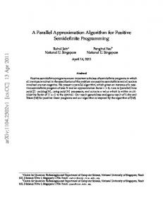
Given a complete graph G0 = (V, E) with metric edge costs and |V | ≥ 3, equality holds in Lemma 1 for the special case where ri = k = 2 for all i ∈ V . This is shown by Alexander, Boyd, and Elliott-Magwood [2] in their Lemma 3. In other words, when the edge costs are metric in a complete graph G0 = (V, E) with |V | ≥ 3, we have that opt(multi-2EC on G0 ) = opt(2EC on G0 ). It is important to note that equality in Lemma 1 does not hold in general. In fact, equality does not even hold in general for kEC and multi-kEC for k > 2, even for metric edge costs. For example, take the family of complete graphs on k + 1 vertices, k > 2. Arrange the vertices in a circle. Assign edge costs 1 to all the “outside” edges, and edge cost 2 to all the “inside” edges. These edge costs are metric. The optimal kEC solution is the graph itself, with total cost 1(k + 1) + 2[ (k−2)(k+1) ] = k 2 − 1. An optimal multi-kEC solution, k even, is 2 k obtained by taking 2 copies of all the outside edges, with total cost k2 (k + 1) < k 2 − 1. An optimal multi-kEC solution, k odd, is obtained by taking k+1 2 copies k+1 of k of the outside edges and ( 2 ) − 1 copies of the remaining outside edge, k+1 1 2 2 with total cost ( k+1 2 )(k) + [( 2 ) − 1] = 2 (k + 2k − 1) < k − 1. Thus, for this family of graphs with metric edge costs and k > 2, opt(multi-kEC) < opt(kEC). Figure 1 illustrates this family of graphs for k = 3. In 2006, Alexander, Boyd, and Elliott-Magwood showed that the integrality gap of the LP relaxation of multi-2EC (and metric 2EC) is ≤ 3/2 [2], and 20

1 1

2 2

1

1 1

1

1

2 2

1

1

1

opt(multi−3EC on G’) = 7

opt(metric 3EC on G’) = 8

1 G’

1

Figure 1: k = 3 in the family of graphs.

showed the exact integrality gap for graphs of up to 10 vertices, and a tight lower bound for the integrality gap for graphs of 11 to 14 vertices. In both [3] and [2], it is mentioned that examples exist with an integrality gap ratio which asymptotically approaches 6/5, thus indicating that the integrality gap for the LP relaxation of multi-2EC (and metric 2EC) is between 6/5 and 3/2. In 1998, Carr and Ravi [3] conjectured that the integrality gap is in fact 4/3, and presented a result that provides some support for this. In 1982, Frederickson and Ja’Ja’ presented a 3/2-approximation algorithm that applies to metric 2EC [10]. Note that when edge costs are metric, k = 2, and there are at least three vertices in the graph, Alexander, Boyd, and Elliott-Magwood [2] show that there is always an optimal solution of multi-2EC that is simple. In other words, given a complete graph G0 = (V, E), with |V | ≥ 3 and with metric edge costs c0 ∈ RE , opt(multi-2EC on G0 ) =

opt(metric 2EC on G0 ).

(28)

Problems multi-2EC and metric 2EC are closely related. This is shown by the following proposition. Proposition 6 Given a complete graph G = (V, E), |V | ≥ 3, with non-negative edge costs c ∈ RE , let G4 = (V, E) be the metric completion of G, with metric costs c4 ∈ RE . Then opt(multi-2EC on G) = opt(metric 2EC on G4 ). Proof: Set k = 2 in Corollary 2 and apply equation (28) with G0 = G4 . ¥ It is interesting to note that, for graphs that are their own metric completion, there is a relationship between the integrality gaps for the linear programming relaxation of multi-2EC and for the linear programming relaxation of metric 2EC. Lemma 4 Given a complete graph G0 = (V, E), |V | ≥ 3, with metric edge costs c0 ∈ RE , if the metric completion G4 is the same as G0 , i.e., if G4 = G0 , then the integrality gap for the linear programming relaxation of multi-2EC on G0 is less than or equal to the integrality gap for the linear programming relaxation of metric 2EC on G0 . Proof: By Lemma 1, opt(multi-2EC on G0 )

≤ opt(metric 2EC on G0 ). 21

By equation (28), opt(multi-2EC on G0 ) = opt(metric 2EC on G0 ). Hence, opt(multi-2ECLP on G0 ) = opt(metric 2ECLP on G0 ). We therefore have that opt(multi-2EC on G0 ) opt(multi-2ECLP on G0 )

≤

opt(metric 2EC on G0 ) . opt(metric 2ECLP on G0 )

¥ The following lemma comes from equation (28) and the proof of Theorem 4. It agrees with a result presented by Alexander, Boyd, and Elliott-Magwood [2]. Lemma 5 Given a complete graph G0 = (V, E), |V | ≥ 3, with metric edge costs c0 ∈ RE , the integrality gap for the linear programming relaxation of metric 2EC is at most 32 . A graph is said to be k-vertex connected if it has at least k internally vertexdisjoint paths between every pair of vertices. All k-vertex connected graphs are k-edge connected, but not vice versa. Given a complete graph, G = (V, E), with non-negative edge costs c ∈ RE , the k-vertex connected subgraph problem (kVC) is the problem of finding a minimum cost k-vertex connected spanning subgraph of G. Problem 2VC is sometimes called the biconnected augmentation problem. Problem kVC with metric edge costs will be referred to as metric kVC. For a summary of the current known performance guarantees on the different versions of kVC, see [21]. It can be shown that opt(metric 2EC) = opt(metric 2V C). This is an implicit result of Frederickson and Ja’Ja”s shortcutting method (cf [10]), and is used by Carr and Ravi in [3], and by Monma, Munson, and Pulleyblank in [23]. In 1982, Frederickson and Ja’Ja’ examined the biconnected augmentation problem on complete graphs with metric edge costs and F = ∅ [10], i.e., metric 2VC. Following a similar idea to that of Christofides’ 32 -approximation algorithm for the metric travelling salesman problem [5], Frederickson and Ja’Ja’ presented a 23 -approximation algorithm for metric 2EC and metric 2VC. Given a complete graph G0 = (V, E) with metric edge costs, our approximation algorithm for multi-kEC in Section 3 can be modified to get a 32 approximation algorithm for metric 2EC that is similar to that of Frederickson ˆ be the heurisand Ja’Ja”s. The modification is as follows: Set k = 2 and let H tic solution obtained from our approximation algorithm (cf Section 3) applied ˆ is a 2-edge connected spanning multi-subgraph. Also note to G0 . Note that H ˆ consist of exactly two parallel edges. (Otherwise, we that any multi-edges of H can remove at least one copy of the parallel edges without affecting the 2-edge connectivity, thus obtaining a cheaper solution.) We can remove the parallel ˆ as follows [10]: For each edge uv in J 0 ∩ E 0 : (a) remove uv from J 0 ; edges of H (b) find an adjacent edge ux or vw in E 0 , remove it from E 0 and replace it with either vx or uw, respectively; (c) insert the remaining edges of J 0 into E 0 , and ˜ Form the simple subgraph H ˜ = (V, E). ˜ call this combined set of edges E. Corollary 7 Given a complete graph G0 = (V, E), |V | ≥ 3, with metric edge costs c0 ∈ RE , the approximation algorithm from Section 3 (with k = 2), with 22

the addition of the above transformation as step (A4), is a algorithm for metric 2EC.

3 2 -approximation

ˆ be the heuristic solution obtained from the apProof: Set k = 2 and let H ˜ be the resulting proximation algorithm from Section 3 applied to G0 . Let H ˆ subgraph after applying the above transformation to H. ˆ have even degree. Without Note that, by construction, all the vertices of H loss of generality, assume that the edge ux is removed along with uv in the step (A4) above, and xv is added. The degree of u decreases by two, and the degree of x and v remain the same. Since the vertex u was incident with the parallel edge uv and the edge ux, and its degree was even, therefore the degree of u was greater than or equal to four. Thus, decreasing the degree of u by two does not disconnect u from the graph. Hence, the resulting subgraph is connected and still has vertices of all even degree. As well, no new parallel edges are created, ˆ (if xv were in E 0 then (V, E 0 ) would contain a since the edge xv is not in H cycle (cycle xuvx) and thus would not be a minimum spanning tree; and if xv were in J 0 then J 0 would not be a T -join for T = V 0 ). Repeating for each of the ˆ we see that the resulting subgraph H ˜ is connected and has parallel edges of H, ˜ ˜ is also simple. vertices of all even degree. Hence, H is 2-edge connected. H Due to metric costs, the transformation of step (A4) is performed at no ˜ is a 2-edge connected spanning simple increase in total edge cost. Thus, H 3 0 subgraph of G with cost at most 2 opt(metric 2EC). Since step (A4) can also be done in polynomial time, this yields a 32 -approximation algorithm for metric 2EC. ¥ ˜ to Note that if, furthermore, we wish the metric 2EC heuristic solution H be 2-vertex connected, then we apply Frederickson and Ja’Ja”s shortcutting method [10] to obtain at equal cost (due to metric costs) a 2-vertex connected ˜ spanning simple subgraph in the following manner: Choose a cut vertex v of H ˜ such that u and w are in different blocks (maximal and find edges uv and vw in E two-vertex connected components of the graph). Replace uv and vw by uw ∈ E. The blocks containing u and w will then become one block. Repeat until all the blocks of the subgraph are merged and no cut vertices remain. This forms a 23 -approximation algorithm for metric 2VC. The proof of our approximation algorithm for this case provides an alternate, simpler, and more compact proof for Frederickson and Ja’Ja”s result. It is also worthwhile noting that, given a complete graph G = (V, E) with non-negative edge costs, a 32 -approximation algorithm for multi-2EC can be obtained by taking the metric completion G4 of G, applying Frederickson and Ja’Ja”s 32 -approximation algorithm for metric 2EC [10], and then using the transformation by Goemans and Bertsimas in the proof of their Theorem 3 [16], to transform the heuristic solution on G4 back to a heuristic solution on G at no increase in cost and no decrease in edge connectivity.

23

7

Acknowledgment

This research was partially supported by grants from the National Sciences and Engineering Research Council of Canada.

References [1] M. Aggarwal and N. Garg, A Scaling Technique for Better Network Design, Proc. of the 5th annual ACM-SIAM Symposium on Discrete Algorithms (1994) 233-240. [2] A. Alexander, S. Boyd, P. Elliott-Magwood, On the Integrality Gap of the 2-Edge Connected Subgraph Problem, Technical Report TR-2006-04, S.I.T.E., University of Ottawa, Ottawa, 2006. [3] R. Carr, R. Ravi, A New Bound for the 2-Edge Connected Subgraph Problem, Lecture Notes in Computer Science 1412 (1998) 112-125. [4] S. Chopra, On the Spanning Tree Polyhedron, Operations Research Letters 8 (1989) 25-29. [5] N. Christofides, Worst case analysis of a new heuristic for the traveling salesman problem, Report 388, Graduate School of Industrial Administration, Carneigie Mellon University, Pittsburgh, 1976. [6] W.J. Cook, W.H. Cunningham, W.R. Pulleyblank, A. Shrijver, Combinatorial Optimization, Wiley Interscience, 1998 (Section 5.4). [7] W. Cook, A. Rohe, Computing Minimum Weight Perfect Matchings, Informs Journal on Computing 11 (1999) 138-148. [8] J. Edmonds, E.L. Johnson, Matching, Euler Tours and the Chinese Postman, Math. Prog. 5 (1973) 88-124. [9] K.P. Eswaran, R.E. Tarjan, Augmentation Problems, SIAM J. Comput. 5 (1976) 653-665. [10] G.N. Frederickson, J. Ja’Ja’, On the relationship between the biconnectivity augmentation and travelling salesman problems, Theoretical Computer Science 19 (1982) 189-201. [11] M.L. Fredman, R.E. Tarjan, Fibonacci Heaps and Their Uses in Improved Network Optimization Algorithms, Journal of the Association for Computing Machinery 34 No.3 (1987) 596-615. [12] H.N. Gabow, An ear decomposition approach to approximating the smallest 3-edge connected spanning subgraph of a multigraph, SIAM J. Discrete Math. 18 No.1 (2004) 41-70.

24

[13] H.N. Gabow, M.X. Goemans, E. Tardos, D.P. Williamson, Approximating the smallest k-edge connected spanning subgraph by LP-rounding, Proceedings of the sixteenth annual ACM-SIAM symposium on Discrete algorithms (2005) 562-571. [14] H.N. Gabow, M.X. Goemans, D.P. Williamson, An efficient approximation algorithm for the survivable network design problem, Mathematical Programming 82 (1998) 13-40. [15] M.R. Garey, D.S. Johnson, Computers and Intractability: A Guide to the Theory of NP-Completeness, W. H. Freeman & Co., New York, NY (1979). [16] M.X. Goemans and D.J. Bertsimas, Survivable networks, linear programming relaxations and the parsimonious property, Mathematical Programming 60 (June 1993) 145-166. [17] M. Gr¨otschel, C.L. Monma, M. Stoer, Design of Survivable Networks, in: M.O. Bell, T.L. Magnant, C.L. Monma, G.L. Nemhauser, eds, Network Models (Handbooks in OR & MS, Vol.7), North-Holland, 1995. [18] K. Jain, A Factor 2 Approximation Algorithm for the Generalized Steiner Network Problem, Combinatorica 21 No.1 (2001) 39-60. [19] R.M. Karp, Reducibility among combinatorial problems, in: R.E. Miller, J.W. Thatcher, eds, Complexity of computer computations, Plenum Press (NY), 1972, 85-104. [20] S. Khuller and U. Vishkin, Biconnectivity approximations and graph carvings, Journal of the ACM 41 (1994) 214-235. Preliminary version in Proc. 24th Annual ACM Symp. on Theory of Computing (1992) 759-770. [21] G. Kortsarz, Z. Nutov, Approximating Minimum-Cost Connectivity Problems, in: T.F. Gonzalez, ed., Handbook of Approximation Algorithms and Metaheuristics, Chapman & Hall, 2007. [22] L. Lov´asz, et. al., Combinatorics in computer science, in: R.L. Graham, M. Gr¨otschel, L. Lov´asz, eds., Handbook of Combinatorics Volume II, Elsevier Science, 1995. [23] C.L. Monma, B.S. Munson, W.R. Pulleyblank, Minimum-weight twoconnected spanning networks, Math. Prog. 46 (1990) 153-171. [24] V.V. Vazirani, Recent results on approximating the Steiner tree problem and its generalizations, Theoretical Computer Science 235 (2000) 205-216.

25