Inter-Layer Bit-Allocation for Scalable Video Coding - IIS, SINICA

1

Inter-Layer Bit-Allocation for Scalable Video Coding Guan-Ju Peng, Member, IEEE, Wen-Liang Hwang, Senior Member, IEEE, and Sao-Jie Chen, Senior Member, IEEE

Abstract—In this paper, we present a theoretical analysis of the distortion in multi-layer coding structures. Specifically, we analyze the prediction structure used to achieve temporal, spatial, and quality scalability of scalable video coding (SVC), and show that the average peak-signal-to-noise (PSNR) of SVC is a weighted combination of the bit rates assigned to all the streams. Our analysis utilizes the end user’s preference for certain resolutions. We also propose a rate-distortion (RD) optimization algorithm, and compare its performance with that of a state-of-the-art scalable bit allocation algorithm. The reported experiment results demonstrate that the R-D algorithm significantly outperforms the compared approach in terms of the average PSNR.

I. I NTRODUCTION Scalable video coding (SVC) facilitates the encoding of a bitstream containing representations with lower spatial resolutions, frame rates, and quality, which are designed to meet the requirements of the heterogeneous display and computational capabilities of the target devices. A client with restricted resources (display resolution, processing power and bandwidth) can only decode a part of the delivered bitstream. Thus, SVC can be used in wide range of multicast applications, such as Internet and wireless applications, where scalability is necessary in order to deal with the variable transmission conditions to the end users. Another benefit of SVC is that it can adapt to a network-aware environment on-the-fly [1], [2] when feedback is provided by the network and the end users. H.264/SVC is a state-of-the art SVC codec that significantly reduces the gap in rate-distortion (R-D) efficiency between state-of-the art signal layer coding and scalable coding [3], [4]. The performance of SVC depends to a large extent on the settings of several parameters [5]. The quantization parameters (QP ), the ratio of the I, P , and B frames, and the target bit rate have the most influence on the performance. In this paper, we study the multiple-layer bit rate allocation problem in SVC, also known as the optimal quantization parameter (QP ) assignment to each layer in SVC. With the objective of simplifying the analysis without affecting its generality, we fix the values of several SVC coding parameters. Specifically, we assume that the motion vectors have been acquired already. In addition, we use the hierarchical B-frame structure for temporal scalability and inter-layer residual prediction for spatial and coarse-grain quality scalability [4]. Guan-Ju Peng and Sao-Jie Chen are with the Graduate Institute of Electronic Engineering, National Taiwan University, Taipei, Taiwan. Wen-Liang Hwang is with the Institute of Information Science, Academia Sinica, Taipei, Taiwan.

The optimal bit allocation of a rate-constrained encoder control system is usually derived by applying the Lagrangian technique [6]. In contrast to single-layer video coding, SVC requires that all users are served simultaneously in a single bitstream. Thus, the data items in an SVC bitstream are highly correlated to each other. This inter-dependency can cause a coding error in one layer to propagate to other layers and thereby complicate the bit allocation process. Another factor that affects bit allocation under SVC is the end user’s preference. For example, the bit allocation scheme for users subscribing to the highest resolution should be different from that for users subscribing to the lowest resolution, since the latter only uses the base layer information. Hence, the preferences for some resolutions should also be considered by the bit allocation scheme. However, incorporating users’ preferences into the bit allocation process implies that the preference information should be acquired by the encoder through a feedback mechanism. This is usually considered a disadvantage in a broadcasting environment. Ramchandran, Ortega, and Vitterli [7] studied bit allocation in a multi-layer coding environment. They model the distortion in all layers as a weighted average of the distortions of the layers, and then use R-D optimization based on the Lagrangian technique to optimize the weighted distortion. In [8], Schwartz and Wiegand propose an encoder control mechanism that jointly optimizes the coding parameters of the base layer and enhancement layers under H.264/SVC. Their algorithm also utilizes a weighted combination of the distortions of all the layers to balance the coding efficiency of different layers. Although the above approaches demonstrate the correlation between the coding performance and the values of the weighting factors, analyses of the derivation of the weighting factors are not provided. Recently, Koziri and Eleftheriadis [9] presented an interesting approach that models the distortion dependency between layers as a stochastic process for joint optimization of scalable coding. However, their analysis is limited to Gaussian sources and spatial dependency. In this paper, we propose a theoretical analysis of the weighting factor approach for joint optimization of scalable coding. We analyze the effect of a coding error in one layer on the other layers in terms of the residual prediction of temporal, spatial, and quality scalability under SVC. Then, we demonstrate that the weighting factor of a layer i is a function of all the layers affected by the coding error in layer i, and the end user’s preference for subscribing to the affected layers. Based on the analysis, we derive the main result, namely, the average PSNR can be represented as the

2

weighted combination of the bit rate assigned to each layer, where the coefficient is the weighting factor. We also propose an R-D optimization algorithm. Experiments on H.264/SVC JSVM 9.18 [10] demonstrate that the algorithm achieves a significant improvement over the state-of-the-art method [8], [7] in terms of the average PSNR. The remainder of this paper is organized as follows. In the next section, we consider several issues that are relevant to bit allocation under SVC. In Section III, we analyze the coding error of the predicting frames and the predicted frame in two adjacent layers; and in Section IV, we extend the derived result to all the frames in adjacent layers. In Section V, we derive the R-D function of SVC; and in Section VI, we present our algorithm for solving the optimal bit allocation problem in SVC. We discuss a number of implementation issues and the experimental results in Section VII; and then summarize our conclusions in Section VIII.

B. Quality measurement of SVC To assess the performance of the multi-layer structure, we use the model proposed in [12]. Suppose there are N subscribers, from 1 to N , and the video quality they receive is measured by the peak-signal-to-noise ratio, i.e., P SN R1 , P SN R2 , P SN R3 , ..., P SN RN , respectively. We also introduce the parameter ψi to denote the preference of subscriber i in the system. ∑N Then, the overall quality of the N subscriber system is i=1 ψi P SN Ri . A scalable codec supports several spatial, temporal, and quality resolutions. Let S, T and R represent the sets of spatial, temporal, and quality resolutions, respectively; and let [s, t, r] denote a particular resolution with s ∈ S, t ∈ T , and r ∈ R. In addition, let q(i) denote the resolution that subscriber i requests. Based on the subscribers to the resolution [s, t, r], we have QN

=

i=1

II. A SPECTS OF THE SVC B IT- ALLOCATION P ROBLEM In this section, we discuss three important aspects of the SVC bit-allocation method for a scalable video codec, namely, the R-D model, the measurement of the source coder’s performance, and the structure of data dependency under SVC.

=

R(ρ) = θ(1 − ρ),

(1)

D(ρ) = σ 2 e−α(1−ρ) ,

(2)

where D represents the mean-square-error (MSE). Substituting Equation (1) into Equation (2), we obtain the result such that D(R)

P SN R

∑

P SN R[s,t,r]

ψi .

(6)

q(i)=[s,t,r]

ψi =

∑

∑

ψi ,

(7)

s∈S,t∈T,r∈R q(i)=[s,t,r]

we obtain the average PSNR: ∑ ¯ R = P SN

µ[s,t,r] P SN R[s,t,r] ,

(8)

s∈S,t∈T,r∈R

where the preference factor of the [s, t, r] resolution is ∑ q(i)=[s,t,r] ψi ∑ , µ[s,t,r] = ∑ s∈S,t∈T,r∈R q(i)=[s,t,r] ψi

(9)

which represents the proportion of preferences for the resolution [s, t, r]. If we replace the PSNR in Equation(8) by 2552 10 ∑ log10 D and use the facts that 0 ≤ µ[s,t,r] ≤ 1 and s∈S,t∈T,r∈R µ[s,t,r] = 1, we obtain ∏ µ[s,t,r] ¯ R = 10 log10 2552 − 10 log10 P SN D[s,t,r] . s∈S,t∈T,r∈R

= σ 2 e−Rγ ,

and γ = α/θ. The parameter γ is propositional to

∑

If we normalize QN by dividing it by the preferences of all subscribers; i.e.,

i=1

In our analysis, we use He and Mitra’s ρ-domain source model [11], which relates the number of zeros to the ratedistortion function of quantized DCT coefficients. Let ρ denote the percentage of zeros in the quantized DCT coefficients. In the model, the rate R is linearly dependent on ρ and the distortion D is exponentially dependent on ρ. The relations are shown in the following equations in which α and θ are parameters and σ is the picture variance:

ψi P SN Rq(i)

s∈S,t∈T,r∈R

N ∑

A. The rate-distortion model

N ∑

(3) dP SN R : dR

= 10 log10 2552 − 10 log10 e ln D 2552 = 10 log10 2 + (10 log10 e)γR. σ

(4) (5)

Equation (5) is obtained by substituting Equation (2) into Equation (4). He and Mitra’s model assumes that γ is a constant; however, if γ is a constant, then, according to Equation (5), the PSNR and R are linearly related. This model is usually correct at high bit rates, but not so exact at low bit rates. Thus, we assume that the value of γ changes slowly with respect to R and can be approximated as a constant at high bit rates.

(10) Equation (10) indicates that the maximization of the average PSNR can be obtained by minimizing ∏ µ[s,t,r] D[s,t,r] . (11) s∈S,t∈T,r∈R

C. Layer dependency and the sequence of approximations To achieve high quality scalability, SVC usually encodes data into different layers of granularity. Recall that S, T and R represent the spatial, temporal, and quality layer identifiers respectively; and let (s, l, r) denote a particular stream in which the spatial layer identifer s ∈ S, the temporal level identifer l ∈ T , and the quality layer identifier r ∈ R. In this paper, we do not distinguish between layers and resolutions.

3

However, temporal layer l and temporal level l have different meanings [4]. Specifically, temporal layer l contains all the frames in temporal levels 0, 1, · · · , l; and temporal level l only contains the frames in that level. The data dependency structure can be represented by a directed graph G = (V, E) with a vertex set V and an edge set E = V ×V . A directed edge uv ⃗ indicates that the edge is from vertex u to vertex v, but not from v to u. In SVC, a stream is represented by a vertex and the dependency between two streams is represented by an edge between their corresponding vertices. A directed edge from the stream (s, l, r) to the stream (s′ , l′ , r′ ) indicates that the data in (s′ , l′ , r′ ) is predicted based on the data in (s, l, r). We assume that the elements in S, T , and R can be enumerated as S = {0, 1, · · · , |S| − 1}, T = {0, 1, · · · , |T | − 1}, and R = {1, · · · , |R|}. In addition, we assume that SVC has the following prediction structure. The data in the stream (s, l, r) can be used to predict the data in streams (s + 1, l, r) (spatial prediction), (s, l, r + 1) (quality prediction), and (s, l + 1, r) (temporal prediction), provided that s + 1 < S, r ≤ R, and l + 1 < T . If the edge is defined accordingly, the directed graph is a directed acyclic graph that does not have cycles and any vertex (s, l, r) can be reached from (0, 0, 1). In H.264/SVC, the coarse-grain quality prediction has a particular structure, as shown in Figure 1. The data in the stream (s, l, r) with r < |R| predicts that in the stream (s, l, r + 1); meanwhile, the data in the stream (s, l, |R|) predicts that of stream (s + 1, l, 1). We use Ii,(s,l,∞) to indicate that the input frame i is of spatial resolution s, is in temporal level l. The coarsest approximation of Ii,(s,t,∞) is Ii,(s,t,1) , which is the reconstructed frame with one quality layer, and the next coarsest approximation is Ii,(s,t,2) , reconstructed with the first two quality layers, and so on. Thus, from coarse to fine, the sequence of approximation of Ii,(s,l,∞) is Ii,(s,l,1) , Ii,(s,l,2) , · · · . To derive the coding error of the input frame Ii,(s,l,∞) , we need to examine the error that occurs in each prediction stage in Figure 1 and its propagation to the other prediction stages. III. P REDICTION R ESIDUALS AND D ISTORTION P ROPAGATION In this section, we derive the prediction residuals of different types of data predictions, as well as the relations between the distortion of the predicted frame in one stream and that of the predicting frames in another stream. A. Prediction residuals In the derivations, we use a column vector to represent a frame, and assume that the motion vectors have been obtained. If ∆i,(s,l,r) represents the coding error between Ii,(s,l,∞) and Ii,(s,l,r) , we have Ii,(s,l,r) = Ii,(s,l,∞) − ∆i,(s,l,r) ,

(12)

where Ii,(s,l,r) is the reconstructed frame at the quality layer r. Note that ∆i,(s,l,r) decreases as the quality layer r increases. Notations In SVC, an input frame is subjected to temporal prediction, spatial prediction, and quality prediction. Thus, the notation

used to represent an object must specify the prediction sequence applied to obtain the object. We use the following notations to represent objects:

1.

2.

3.

r,t Xi,(s,l) denotes an object X associated with frame i of spatial resolution s and temporal level l. The object is derived by applying temporal prediction to the input frame Ii,(s,l,∞) with the predicting frames of quality resolution r. For example, if X = I, r,t then Ii,(s,l) is the predicted frame of Ii,(s,l,∞) when Ii,(s,l,∞) is temporally predicted with the predicting frames of quality resolution r. If X = ∆, where ∆ is the prediction residual, then ∆r,t i,(s,l) denotes the residual obtained after applying temporal prediction to Ii,(s,l,∞) with the predicting frames of quality resolution r. Similarly, if X = C and C is a constant, r,t then Ci,(s,l) denotes the derived constant obtained in a similar way. r,s Xi,(s,l) denotes an object X associated with frame i of spatial resolution s and temporal level l. The object is derived by applying temporal and spatial prediction to the input frame Ii,(s,l,∞) with the predicting frames of quality resolution r. If X = I, r,s then Ii,(s,l) is the predicted frame of Ii,(s,l,∞) when Ii,(s,l,∞) is temporally and spatially predicted with the predicting frames of quality resolution r. If X = ∆, where ∆ is the prediction residual, then ∆r,s i,(s,l) is the residual obtained after temporal and spatial prediction of Ii,(s,l,∞) with the predicting frames of quality resolution r. Similarly, if X = C r,s and C is a constant, then Ci,(s,l) denotes the derived constant. r,q Xi,(s,l) denotes an object X obtained by applying temporal prediction and quality prediction to the input frame Ii,(s,l,∞) with the predicting frames of r,q quality resolution r. If X = I, then Ii,(s,l) is the resulting predicted frame of Ii,(s,l,∞) ; and if X = ∆, where ∆ is the residual, then ∆r,q i,(s,l) is the resulting residual. Similarly, if X = C and C is a constant, r,q then Ci,(s,l) is the derived constant.

r,s Following Equation (12), the residuals ∆r,t i,(s,l) , ∆i,(s,l) , and r,t ∆r,q i,(s,l) can be represented as Ii,(s,l,∞) − Ii,(s,l) , Ii,(s,l,∞) − r,q r,s Ii,(s,l) , and Ii,(s,l,∞) − Ii,(s,l) , respectively.

A. Temporal prediction In SVC, temporal scalability with dyadic temporal levels can be implemented effectively by a hierarchical prediction structure. In temporal prediction, the macroblocks of the input frame Ii,(s,l,∞) can be either INTER- or INTRA- predicted. The INTER macroblocks are predicted by the corresponding reconstructed frames, Ii−m,(s,l−1,r) and Ii+m,(s,l−1,r) , with l ≥ 1. Let Ar,t i,(s,l) denote the pixels predicted in INTRA r,t macroblocks; then, Ii,(s,l) , as defined in Notation 1 is obtained

4

(12) for Ii,(s−1,l,|R|) and Equation (15) for ∆1,t i,(s,l) , we obtain

by

=

∆r,t i,(s,l) Ii,(s,l,∞) − {Pi,i−m Ii−m,(s,l−1,r) + Pi,i+m Ii+m,(s,l−1,r) } − Ar,t i,(s,l)

=

∆1,s i,(s,l) =

(Pi,i−m ∆i−m,(s,l−1,1) + Pi,i+m ∆i+m,(s,l−1,1) ) −Ar,s i,(s,l) ) −

(13)

(Ii,(s,l,∞) − Pi,i−m Ii−m,(s,l−1,∞) −Pi,i+m Ii+m,(s,l−1,∞) −

Ar,t i,(s,l) )

|R|,q

U (Ii,(s−1,l,∞) − ∆i,(s−1,l,|R|) − Ii,(s−1,l) ) +

=

(Pi,i−m ∆i−m,(s,l−1,r) + Pi,i+m ∆i+m,(s,l−1,r) ) r,t Ci,(s,l) +

(Pi,i−m ∆i−m,(s,l−1,r) + Pi,i+m ∆i+m,(s,l−1,r) ), (15) where P is the matrix representation of the motion compensar,t tion prediction method for IN T ER macroblocks, and Ci,(s,l) is the constant error, as defined in Notation 1. The second term in Equation (15) represents the propagation of the residuals ∆i−m,(s,l−1,r) and ∆i+m,(s,l−1,r) of the reconstructed predicting frames in the previous temporal level. If we assume that the first and second terms in Equation (15) are uncorrelated, then we have

1,t (Ci,(s,l)

−

|R|,q U (∆i,(s−1,l) )

−

Ar,s i,(s,l) )

(18)

+

(Pi,i−m ∆i−m,(s,l−1,1) + Pi,i+m ∆i+m,(s,l−1,1) ) +U (∆i,(s−1,l,|R|) ) (19)

(14) =

1,t (Ci,(s,l) +

=

1,s Ci,(s,l) +

(Pi,i−m ∆i−m,(s,l−1,1) + Pi,i+m ∆i+m,(s,l−1,1) ) + U (∆i,(s−1,l,|R|) ),

(20)

r,s Ci,(s,l)

where the first term is the constant, the second term is the error propagated from (s, l −1, r), and the third term is the error propagated from (s − 1, l, r). Assuming these terms are uncorrelated, for the streams with s > 0 and r = 1 (only temporal prediction and spatial prediction are applied), the variance of the residual ∆1,s i,(s,l) is 2 σi,(s,l,1) 1,s = var(Ci,(s,l) )+

r,t 2 σi,(s,l,r) = var(Ci,(s,r) )+

var(Pi,i−m ∆i−m,(s,l−1,1) + Pi,i+m ∆i+m,(s,l−1,1) ) +var(U (∆i,(s−1,l,|R|) )). (21)

var(Pi,i−m ∆i−m,(s,l−1,r) + Pi,i+m ∆i+m,(s,l−1,r) ). (16) 2 Note that σi,(s,l,r) is the variance, which is used as part of the distortion calculation by the ρ-domain source model shown in Equation (3). B. Spatial prediction Although spatial prediction is sometimes referred to as INTRA prediction, in this paper, it means prediction based on the information about the video at a lower spatial resolution. Spatial prediction of the INTER macroblocks is achieved by inter-layer spatial residual prediction, which predicts a temporal residual by up-sampling the corresponding reconstructed temporal residual in the previous spatial resolution. We use the matrix U to denote an up-sampling method applied to macroblocks in a frame. If a macroblock is not IN T ER-predicted, it can be predicted by either IN T RA prediction or interlayer intra prediction. Since IN T RA-predicted macroblocks have been considered, we only need to take the inter-layer intra predicted macroblocks into account. Let Ar,s i,(s,l) denote the predicted pixels in the macroblocks to which inter-layer intra-prediction is applied. The residual ∆1,s i,(s,l) , as defined in Notation 2, can be derived with s ≥ 1 as follows: |R|,q

1,t r,s ∆1,s i,(s,l) = ∆i,(s,l) −U (Ii,(s−1,l,|R|) −Ii,(s−1,l) )−Ai,(s,l) , (17)

where the first term is the temporal residual in Equation (15); and the second term is the up-sampled reconstructed residual of the macroblocks, where inter-layer residual prediction is applied in frame i in (s−1, l, |R|). This equation indicates that the residual ∆1,t i,(s,l) is being predicted. Substituting Equation

C. Quality prediction Coarse-grain quality prediction of H.264/SVC is similar to spatial prediction after removing the up-sampling operator in Equation (17). We use the matrix Y to select the pixels used by inter-layer residual prediction. Let Ar,q i,(s,l) denote the pixels in the macroblocks predicted by inter-layer intra prediction; then, the residual ∆r,q i,(s,l) (as defined in Notation 3) with r ≥ 2 can be represented as follows: ∆r,q i,(s,l) =

r,t (Ii,(s,l,∞) − Ii,(s,l) )− r−1,q Y (Ii,(s,l,r−1) − Ii,(s,l) ) − Ar,q i,(s,l)

= =

(∆r,t i,(s,l) ) − r,t (Ci,(s,l) +

Y (Ii,(s,l,r−1) −

r−1,q Ii,(s,l) )

(22) −

Ar,q i,(s,l)

(Pi,i−m ∆i−m,(s,l−1,r) + Pi,i+m ∆i+m,(s,l−1,r) )) +Y (∆i,(s,l,r−1) ) − Ar,q i,(s,l) =

r,t (Ci,(s,l) − Ar,q i,(s,l) ) +

(Pi,i−m ∆i−m,(s,l−1,r) + Pi,i+m ∆i+m,(s,l−1,r) ) +Y (∆i,(s,l,r−1) ) r,q = (Ci,(s,l) )+ (Pi,i−m ∆i−m,(s,l−1,r) + Pi,i+m ∆i+m,(s,l−1,r) ) +Y (∆i,(s,l,r−1) ). r,t Since ∆r,t i,(s,l) = Ii,(s,l,∞) − Ii,(s,l) , the quality prediction is a residual prediction with the residual ∆r,t i,(s,l) being predicted.

5

Similar to Equation (21), the distortion of the residual ∆r,q i,(s,l) can be written as

var(Pi,i−m ∆i−m,(s,l−1,r) + Pi,i+m ∆i+m,(s,l−1,r) ) +var(Y (∆i,(s,l,r−1) )). (23) Although the effects of INTRA prediction and inter-layer intra-prediction are considered in (13), (17), and (22), in the following analysis, we do not take account of the errors propagated to them. Inter-layer intra prediction is applied to macroblocks whose co-located macroblocks in the base layer are IN T RA-predicted. The statistical results indicate that the probability of a macroblock having an INTRA mode in B frames is at most 7% (QP = 50) and 4% on average [13]. As a consequence, we can still derive a good approximation of the optimal rate allocation even when the error propagations of INTRA prediction and inter-layer intra-prediction are excluded. B. Distortion propagation in spatial, temporal, and quality prediction In this sub-section, we explore the relationship between the distortion of the predicted frame and that of the predicting frames. Under H.264/SVC, quality prediction is not applied to quality layer 1, and spatial prediction is not applied to spatial resolution 0. Thus, the derivation of the distortion relationship between the predicting and predicted frames can be divided into three cases: (1) stream (0, l, 1) with l ≥ 1, where only temporal prediction is used; (2) stream (s, l, 1) with s, l ≥ 1, where temporal and spatial prediction are used; and (3) stream (s, l, r) with s, l ≥ 1, r ≥ 2, where temporal and quality prediction are used. Case 1: stream (0, l, 1) with l ≥ 1. Note that the following derivations can also be applied to l = 0, since the stream (0, 0, 1) in the current GOP is temporally predicted by the stream (0, 0, 1) in the previous GOP. In Equation (16), if we substitute 0 and 1 for s and r respectively, we obtain =

1,t var(Ci,(0,l) )

=

2 σi,(0,l,1) 1,t var(Ci,(0,l) )

the value of the indicator function 1{Statement} is 1 if Statement is true, and 0 otherwise. Note that hi,(0,l,1) is a 2 × 1 vector with one of its components set to zero. In a value larger than 0, the component in h is called the dominating term of h because the distortion of the component is larger than that of the other components. Equations (24) and (25) have different interpretations of distortion propagation. Equation (24) indicates that the variance 2 σi,(0,l,1) is contributed by two terms: one from the distortion propagation in the predicting frames, and the other from the coding of the predicted frame. In contrast, Equation (25) indicates that the variance is caused by the distortion propagation in the predicting frames or by encoding of the predicted frame, but not both. Thus, Equation (25) can be regarded as an approximation of Equation (24) by assuming that the variance is propagated from the distortion of the predicting frames or caused by encoding the predicted frame. The approximation greatly simplifies our analysis of distortion propagation in the complex prediction structure of H.264/SVC. In Appendix 1, we provide a simple example to illustrate the approximation’s effect on the analysis of distortion propagation. If the number of bits assigned to encode ∆i−m,(0,l−1,1) and ∆i+m,(0,l−1,1) is small (i.e., a low bit rate), the variance of (Pi,i−m ∆i−m,(0,l−1,1) + Pi,i+m ∆i+m,(0,l−1,1) ) will be large; hence, at a low bit rate, the error of the predicting frames in the previous stream is propagated to and dominates the distortion of the predicted frame in the current stream. On the other hand, if a sufficiently large number of bits are assigned to encode ∆i−m,(0,l−1,1) and ∆i+m,(0,l−1,1) (i.e., a high bit rate), the variance of (Pi,i−m ∆i−m,(0,l−1,1) +Pi,i+m ∆i+m,(0,l−1,1) ) will be small. Thus, at a high bit rate, the error of the predicting frames in the previous stream is irrelevant to the predicted 1,t frame in the current stream because var(Ci,(0,l) ) is a constant. In Appendix 2, we show that, at low bit rates, 2 σi,(0,l,1) ≈ β 1,t ((C α )1,t i−m,(0,l−1) (C )i+m,(0,l−1)

var(Pi,i−m ∆i−m,(0,l−1,1) + Pi,i+m ∆i+m,(0,l−1,1) ).

1

Di−m,(0,l−1,r) Di+m,(0,l−1,r) ) 2 ,

(24) The equation can be re-written as

1,t var(Ci,(0,l) ) var(Pi,i−m ∆i−m,(0,l−1,1) + Pi,i+m ∆i+m,(0,l−1,1) )

=

2 σi,(0,l,1)

+

2 σi,(0,l,1) = hTi,(0,l,1) (

and (κβ )i,(0,l,1)

var(Pi,i−m ∆i−m,(0,l−1,1) +Pi,i+m ∆i+m,(0,l−1,1) ) ;

r,q 2 σi,(s,l,r) = var(Ci,(s,l) )+

2 σi,(0,l,1)

with (κα )i,(0,l,1)

) , (25)

where 1,t hi,(0,l,1) [0] = (κα )i,(0,l,1) 1{var(Ci,(0,l) )≥

var(Pi,i−m ∆i−m,(0,l−1,1) + Pi,i+m ∆i+m,(0,l−1,1) )}; 1,t hi,(0,l,1) [1] = (κβ )i,(0,l,1) 1{var(Ci,(0,l) )
var(Ci,(s,l) ), (32) var(Y (∆i,(s,l,r−1) )) can be approximated as and

var(Pi,i−m ∆i−m,(s,l−1,1) + Pi,i+m ∆i+m,(s,l−1,1) ) ≥ var(U (∆i,(s−1,l,|R|) )). (33) The third component will be non-zero if the predicting frame in stream (s − 1, l, |R|) is assigned a low bit rate; that is, 1,s var(U (∆i,(s−1,l,|R|) )) > var(Ci,(s,l) ),

(34)

and var(U (∆i,(s−1,l,|R|) )) > var(Pi,i−m ∆i−m,(s,l−1,1) + Pi,i+m ∆i+m,(s,l−1,1) ). (35) α

Note that (κ )i,(s,l,1)

=

2 σi,(s,l,1) 1,s var(Ci,(s,l) )

β

, (κ )i,(s,l,1)

2 σi,(s,l,1)

var(Pi,i−m ∆i−m,(s,l−1,1) +Pi,i+m ∆i+m,(s,l−1,1) ) , σ2 (κγ )i,(s,l,1) = var(U (∆i,(s,l,1) . i,(s−1,l,|R|) ))

= and

|R|,s

|R|,s

(38)

where (C ω )r−1,q i,(s,l) depends on the amount of inter-layer residual prediction applied to the macroblocks in ∆i,(s,l,r) . If it is applied to most of the macroblocks in ∆i,(s,l,r) , then (C ω )r−1,q i,(s,l) ≈ 1. 2 We can summarize the three approximations of σi,(s,l,r) as follows: For the frames in stream (0, l, 1) with l ≥ 1, we have 2 T σi,(0,l,1) = hi,(0,l,1) 



 

 .

1,t var(C ) i,(0,l) 1 1,t 1,t α β ((C ) (C ) Di−m,(0,l−1,r) Di+m,(0,l−1,r) ) 2 . i−m,(0,l−1) i+m,(0,l−1)

(39)

For the frames in stream (s, l, 1) with s, l ≥ 1, we have 2 T σi,(s,l,1) = hi,(s,l,1) 

In Appendix 3, we show that, at low bit rates, var(U (∆i,(s−1,l,|R|) )) can be approximated as 2 σi,(s,l,1) = (C ω )i,(s−1,l) Di,(s−1,l,|R|) ,

2 σi,(s,l,r) = (C ω )r−1,q i,(s,l) Di,(s,l,r−1) ,

1,s var(C ) i,(s,l)   1  1,t 1,t  ((C α ) (C β ) Di−m,(s,l−1,1) Di+m,(s,l−1,1) ) 2  i−m,(s,l−1) i+m,(s,l−1)  |R|,s ω (C ) D )) i,(s−1,l) i,(s−1,l,|R|)

   .   (40)

(36)

where (C ω )i,(s−1,l) depends on the up-sampling method employed. If bilinear interpolation is used to up-sample most of |R|,s the macroblocks in ∆i,(s−1,l,|R|) , then (C ω )i,(s−1,l) ≈ 1. Case 3: stream (s, l, r) with s, l ≥ 1 and r ≥ 2. In this case, both temporal prediction and quality prediction are applied to predict a frame, and the variance of the predicted



For the frames in stream (s, l, r) with s, l ≥ 1 and r ≥ 2, we have 2 T σi,(s,l,r) = hi,(s,l,r) 

r,q var(C ) i,(s,l)  1  r,t β  ((C α )r,t (C ) Di−m,(s,l−1,r) Di+m,(s,l−1,r) ) 2  i−m,(s,l−1) i+m,(s,l−1)  r−1,q (C ω ) D i,(s,l) i,(s,l,r−1)

   .   (41)

7

IV. D ISTORTION OF A L AYER We represent the distortion of a stream as a function of the bits assigned to encode the layers along the residual prediction path. Recall that, in our analysis, we adopt the dyadic temporal enhancement layer structure in which the input frames of a group of pictures (GOP) are organized in different temporal levels. We use nu(l) to denote the number of frames in temporal level identifier l. The dyadic temporal enhancement layer structure means that nu(0) = n0 , and nu(l) = 2nu(l − 1) f or l ≥ 1,

(42)

where n0 is the number of frames in the stream (0, 0, 1). For convenience, we define that nu(−1) = 0. The number of frames in temporal level l is 2l−1 n0 . A user who subscribes to temporal resolution t will receive all the frames in the temporal∑level identifiers 0, 1, · · · , t. Thus, the user will t t receive i=0 nu(i) = 2 n0 frames. Note that the number of frames in the temporal layer identifier t differs from the number of frames in the temporal resolution t. If we enumerate the frames from 1 to 2t n0 and divide them into t + 1 temporal layers with identifiers from 0 to t, the frames numbered from 1 to n0 will be assigned to temporal level identifier 0; and the frames numbered from 2l−1 n0 + 1 to 2l n0 will be assigned to temporal layer identifier l, with l ≥ 1. The average distortion of the frames in the resolution [s, t, r], denoted by D[s,t,r] , can be derived by calculating the geometric mean of the frame distortion Di,[s,t,r] as follows: D[s,t,r]

t ∏ =(

∏

nu(l)

1

Di,(s,l,r) ) 2t n0 .

(43)

l=0 i=nu(l−1)+1

Thus, the distortion of the resolution [s, t, r] is the geometric mean of the distortions in stream, (s, 0, r), · · · , (s, t, r). We let nu(l) ∑ b(s,l,r) = bi,(s,l,r) (44)

To derive the distortion of a temporal level that is only temporally predicted, according to Equations (39), (46) and (45), the distortion of (0, l, 1) is

∏

nu(l)

Di,(0,l,1)

i=nu(l−1)+1

∏

nu(l)

=

2 σi,(0,l,1) exp{−γi,(0,l,1) bi,(0,l,1) }

i=nu(l−1)+1

∏

nu(l)

=

hTi,(0,l,1)

i=nu(l−1)+1

(

)

1,t var(C ) i,(0,l) 1 1,t,α 1,t,β (C C D D )2 i−m,(0,l−1) i+m,(0,l−1) i−m,(0,l−1,r) i+m,(0,l−1,r)

exp{−γi,(0,l,1) bi,(0,l,1) }. (47)

Note that each frame in the predicted temporal level l is predicted by two frames in the predicting level l − 1: one for forward prediction and the other for backward prediction. If l ≥ 2, the predicted level will have twice as many frames as the predicting level. Similarly, to derive the distortion of the temporally and spatially predicted stream (s, l, 1), with s ≥ 1, Equations (40), (46) and (45) are used. The distortion of (s, l, 1) can be computed as

i=nu(l−1)+1

∏

nu(l)

denote the total number of bits assigned to the frames in the stream (s, l, r), and ∏

nu(l) 2 σ(s,l,r) =

Di,(s,l,1)

i=nu(l−1)+1 2 σi,(s,l,r)

∏

nu(l)

(45)

=

i=nu(l−1)+1

2 σi,(s,l,1) exp{−γi,(s,l,1) bi,(s,l,1) }

i=nu(l−1)+1

denote the product variance of the frames in the stream (s, l, r). We have analyzed the relationship between the distortion of the predicted frame and that of the predicting frames. In Section IV-A, we extend the results to the distortion between all the frames in the predicting layer and predicted layer. Then, in Section IV-B, we provide an example of error propagation along the prediction path when the referred layers are encoded at low bit rates.

∏

nu(l)

=

hTi,(s,l,1)

i=nu(l−1)+1

 

1,s ) var(C i,(s,l) ((C α )

1 1,t 1,t D D )2 (C β ) i+m,(s,l−1) i−m,(s,l−1,1) i+m,(s,l−1,1) i−m,(s,l−1) |R|,s ω (C ) D i,(s−1,l) i,(s−1,l,|R|)

Di,(s,l,r)

2 = σi,(s,l,r) exp {−γi,(s,l,r) bi,(s,l,r) }.

(46)



exp{−γi,(s,l,1) bi,(s,l,1) }. (48)

A. Prediction error propagation in a temporal level According to the modeling in Equation (3), the distortion of a frame Ii,(s,l,r) is



The distortion of the stream (s, l, r) after quality prediction (r ≥ 2), can be related to the distortion of the frames in

8

streams (s, l − 1, r) and (s, l, r − 1) as follows: ∏

distortion as a function of the bits assigned to an individual stream. Substituting Equation (43) into Equation (11), we have

nu(l)

Di,(s,l,r)

|−1 t ∏ ∏ |T∏ ∏ (

i=nu(l−1)+1

∏

nu(l)

=

r∈R s∈S t=0 2 σi,(s,l,r) exp {−γi,(s,l,r) bi,(s,l,r) }

∏

nu(l)

=

∏

nu(l)

(

r∈R s∈S l=0

µ[s,t,r] 2t n0

∑|T |−1

Di,(s,l,r) )

t=l

µ[s,t,r] 2t n0

.

i=nu(l−1)+1

hTi,(s,l,r)

(51)

i=nu(l−1)+1

(

∏∏ ∏

=

Di,(s,l,r) )

l=0 i=nu(l−1)+1

|T |−1

i=nu(l−1)+1

∏

nu(l)

r,q var(C ) i,(s,l) 1 r,t r,t α β ((C ) (C ) Di−m,(s,l−1,r) Di+m,(s,l−1,r) ) 2 i−m,(s,l−1) i+m,(s,l−1) r−1,q (C ω ) Di,(s,l,r−1) i,(s,l)

exp {−γi,(k,l,r) bi,(k,l,r) }.

) Taking the minus logarithm of Equation (51), we have −

|−1 |T |−1 ∑ ∑ |T∑ ∑ r∈R s∈S l=0

∏

nu(l)

log((

t=l

Di,(s,l,r) )

µ[s,t,r] 2t n0

).

i=nu(l−1)+1

(52) (49) Substituting Equation (50) into Equation (52), the minus In the above derivation, we use the results of Equations (41), logarithm of the average distortion is calculated as (44), (45), and (46). |−1 |T |−1 nu(l) ∑ ∑ |T∑ ∑ µ[s,t,r] ∏ log( Di,(s,l,r) ) B. Exploring error propagation 2t n0 r∈R s∈S l=0 t=l i=nu(l−1)+1 The derivation in Section IV-A can be used to determine the |−1 |T |−1 propagation of the coding error in one stream to other streams. ∑ ∑ |T∑ ∑ µ[s,t,r] = log(C(s,l,r) As mentioned earlier, if a predicting stream is encoded at a 2t n0 high bit rate, its coding error will not be propagated to the r∈R s∈S l=0 t=l predicted stream; on the other hand, if it is encoded at a low nu(l) s ∑ l ∑ r ∑ ∑ bit rate, the coding error can propagate to the predicted stream. exp{ The error propagation can be explored by substituting the k=0 m=0 n=0 i=nu(l−1)+1 distortion in Equation (46) for Di−m,(0,l−1,r) Di+m,(0,l−1,r) (s,l,r) in Equations (47) and (48), Di−m,(0,l−1,r) Di+m,(0,l−1,r) , −ωi,(k,m,n) γi,(k,m,n) bi,(k,m,n) }) Di,(s−1,l,1) in Equation (48), and Di,(s,l,r−1) in Equation (49). |−1 |T |−1 Let us assume that the h value of each frame (which we discuss ∑ ∑ |T∑ ∑ µ[s,t,r] in Section (VI-B)) is known; thus, we know the propagation of {log(C(s,l,r) ) + = 2t n0 the distortion. For a stream (s, l, r), after replacing the model r∈R s∈S l=0 t=l in Equation (46) for the distortion D several times (according nu(l) s ∑ l ∑ r ∑ ∑ to the values of h), the distortion in Equations (47), (48), and (49) can be written as k=0 m=0 n=0 i=nu(l−1)+1

∏

nu(l)

(s,l,r)

−ωi,(k,m,n) γi,(k,m,n) bi,(k,m,n) )}

Di,(s,l,r)

i=nu(l−1)+1

=

C(s,l,r)

s ∏ l r ∏ ∏

∏

nu(m)

=

r∈R s∈S l=0

k=0 m=0 n=0 i=nu(m−1)+1 (s,l,r)

exp{−ωi,(k,m,n) γi,(k,m,n) bi,(k,m,n) } =

+

C(s,l,r) exp{

s ∑ l ∑ r ∑

|−1 |T |−1 ∑ ∑ |T∑ ∑ µ[s,t,r]

(s,l,r)

−ωi,(k,m,n) γi,(k,m,n) bi,(k,m,n) },

k=0 m=0 n=0 i=nu(l−1)+1

2t n0

log C(s,l,r)

|−1 |T |−1 s l ∑ r ∑ ∑ |T∑ ∑ ∑∑ r∈R s∈S l=0

∑

nu(l)

t=l

∑

nu(l)

t=l k=0 m=0 n=0 i=nu(l−1)+1

µ[s,t,r] (s,l,r) ω γi,(k,m,n) bi,(k,m,n) . − t 2 n0 i,(k,m,n) (53)

(50) (s,l,r)

where C(s,l,r) is a constant, and ωi,(k,m,n) is an integer number indicating how many times the distortion Di,(k,m,n) is used to derive the distortion of the stream (s, l, r) in the error propagation process. Based on the results, we can derive the average distortion of SVC.

The first and second terms in Equation (53), denoted by f1 and f2 respectively, can be deduced as follows. 1. The first term: f1

V. T HE AVERAGE D ISTORTION OF SVC Our objective is to determine the optimal bit assignment that will minimize the average distortion function in Equation (11). To achieve the objective, we need to represent the average

=

|−1 |T |−1 ∑ ∑ |T∑ ∑ µ[s,t,r] r∈R s∈S l=0

t=l

2t n0

log C(s,l,r)

(54)

The term represents the constant of the objective function, and is not considered in the bit allocation problem.

9

∑ where Bi is the rate constraint for layer i, and C = i Bi is the maximal rate allowed for encoding the GOP. Note that C and Bi are given values that depend on the user’s bandwidth. The Lagrangian corresponding to the minimization problem (P ) is defined as

2. The second term: f2

=

|−1 |T |−1 s l ∑ r ∑ ∑ |T∑ ∑ ∑∑ r∈R s∈S l=0

=

∑

nu(l)

t=l k=0 m=0 n=0 i=nu(l−1)+1

µ[s,t,r] (s,l,r) ω γi,(k,m,n) bi,(k,m,n) − t 2 n0 i,(k,m,n) |−1 nu(l) ∑ ∑ |T∑ ∑

(55)

L(ξ, λi , bi ) ∑ ∑ ∑ = min − bi wi − λi (Bi − bi ) − ξ(C − bi ), bi

i

i

i

r∈R s∈S l=0 i=nu(l−1)+1

ωi,(s,l,r) γi,(s,l,r) bi,(s,l,r) =

|−1 ∑ ∑ |T∑

ω(s,l,r) b(s,l,r) ,

(57)

r∈R s∈S l=0

where ωi,(s,l,r) denotes the weight of bi,(s,l,r) , which can be calculated by reordering the summations in Equation (55). The value of ω(s,l,r) is the weight of the rate allocated to the stream (s, l, r) and can be computed by ∑nu(l) i=nu(l−1)+1 ωi,(s,l,r) γi,(s,l,r) bi,(s,l,r) ω(s,l,r) = . (58) b(s,l,r) The above derivations and Equation (11) show that maximizing the average PSNR of H.264/SVC with a coarsegrain quality prediction structure can be approximated by maximizing |−1 ∑ ∑ |T∑ ω(s,l,r) b(s,l,r) . (59) r∈R s∈S l=0

VI. S OLVING THE I NTER - LAYER B IT A LLOCATION P ROBLEM Recall that b(k,l,j) represents the number of bits assigned to all the 2l−1 n0 frames in the stream (k, l, j), Thus, Equation (59) represents the inter-layer bit allocation problem in SVC. It is difficult to solve this equation by a direct approach because a weight contains h vectors whose values depend on the results of the bit assignment process. Hence, we solve the problem by finding the optimal bit assignment of a given weight profile instead (see Section VI-A), and then modify the profile based on the derived bit assignment. The proposed optimal bit allocation algorithm is described in Section VI-B. A. Optimal Bit Allocation with Fixed Weights When the weight in Equation (59) is given, finding the optimal bit allocation becomes a constrained linear programming problem. To simplify the formula, we let i = r × |S| × |T | + t × |S| + s. The bit allocation problem involves finding the set of bits {bi |0 ≤ i < |R| × |S| × |T |} that solve the problem (P): |R|×|S|×|T |−1 ∑ (P ) max bi wi , (60) bi

with the constraints { bi ≤ Bi , ∑|R|×|S|×|T |−1 i=0

i=0

∀i bi ≤ C,

(62)

(56)

(61)

where ξ and λi are called Lagrange multipliers. From the Lagrangian, we have { ∑ ∑ − i wi bi if Bi ≥ bi and C ≥ i bi , max L(ξ, λi , bi ) = ∞ otherwise. ξ≥0,λi ≥0 (63) Therefore, the solution of min max L(ξ, λi , bi ) bi

ξ≥0,λi ≥0

(64)

∑ coincides with (P ) in regions where bi ≤ Bi and i bi ≤ C. The duality replaces “min” and “max” in the above equation, resulting in d∗ =

max min L(ξ, λi , bi ) ≤ min max L(ξ, λi , bi ) = p∗ .

ξ≥0,λi ≥0 bi

bi

ξ≥0,λi ≥0

(65) Since L(λ, λi , bi ) is a linear function, and therefore a convex function, and the problem ∑ (P ) has a strictly feasible solution with bi < Bi and i bi < C, according to Slater’s theorem, we have p∗ = d∗ . Thus, the solution of maxλ≥0,λi ≥0 minbi L(ξ, λi , bi ) is the solution of (P ), where minbi L(ξ, λi , bi ) is called the dual function. Let us define the vectors a = (w0 , w1 , · · · , w|R|×|S|×|T |−1 )T , b = (b0 , b1 , · · · , b|R|×|S|×|T |−1 )T , and λ = (λ0 , λ1 , · · · , λ|R|×|S|×|T |−1 )T , where T is the transpose operation. The Lagrangian can be represented as L(ξ, λi , bi ) = −aT b − λT (B − b) − ξ(C − 1T b),

(66)

where 1 is a column vector whose element is 1. Taking the partial derivative of the Lagrangian with respect to b and ξ, we obtain ∂ L(ξ, λi , bi ) = −a + λ + ξ1 = 0, (67) ∂b and ∂ L(ξ, λi , bi ) = C − 1T b = 0, (68) ∂ξ respectively. Solving Equations (67) and (68), we have 1T b = C and λi + ξ = wi with 0 ≤ λi ≤ wi , 0 ≤ ξ ≤ wi . If we let x∗ be mini wi and λ∗i = wi − x∗ , then we have two sets with λ = 0 and λ > 0 as follows: Sλ=0 = {i|λ∗i = 0}; and Sλ>0 = {i|λ∗i > 0}. Substituting the results of Equations (67) and (68) into the Lagrangian, the minimization ∑ of the dual function in the regions where bi ≤ Bi and i bi ≤ C can be written as min ∑

bi ≤Bi ,

i

bi =C

L(ξ, λ∗i , bi ),

(69)

10

such that

VII. I MPLEMENTATION I SSUES AND E XPERIMENTAL R ESULTS

L(ξ, λ∗i , bi ) ∑

=−

{wi bi + λ∗i (Bi − bi )} −

i∈Sλ>0

∑

=−

∑

wi bi

i∈Sλ=0 ∗

(wi Bi − x (Bi − bi )) −

i∈Sλ>0

∑

(70) wi bi .

A. Coding structure and implementation details

i∈Sλ=0

(71) Equation (71) is derived by substituting λ∗i = wi − x∗ into Equation (70). To minimize Equation (71), we choose b∗i = Bi for for i ∈ Sλ>0 . We can then derive that ∑ ∑ min L(ξ, λ∗i , bi ) = − wi Bi − wi bi , ∑ bi ≤Bi ,

i

bi =C

i∈Sλ>0

i∈Sλ=0

(72) ∑

and

∑

Bi +

i∈Sλ>0

bi = C.

(73)

i∈Sλ=0

To minimize Equation (72), we find the optimal solution of ∑ max wi bi (74) bi

i∈Sλ=0

According to the Cauchy Schwarz inequality, the maximum occurs when bi = ϵwi . Thus, we have ∑ ∑ ∑ bi = ϵ wi = C − Bi . (75) i∈Sλ=0

i∈Sλ=0

i∈Sλ>0 ∑ C− i∈S Bi λ>0 ϵ can be computed as ϵ = ∑ . We w i i∈Sλ=0 ∗ the optimal bit allocation bi for a given weight

The value of conclude that profile is { ∑ (C − k∈Sλ>0 Bk ) ∑ wi wk ∗ k∈Sλ=0 bi = Bi

In this section, we consider some implementation issues and compare the performance of QP selection by our method and the method proposed in [7], [8].

Our coding structure, which is a modification of that in [4], supports the selection of QP values during the encoding process, as shown in Figure 2. The implementation is based on H.264/SVC JSVM 9.18. The steps of the encoding process are as follows. The encoder processes one GOP at a time. Before selecting the QP values used in the quantization operation, the modes and motion vectors of the macroblocks in a GOP are computed by the H.264/SVC JSVM 9.18. The M QP s, defined as the QP values used to compute the modes and motion vectors, are obtained from the QP values of the previous GOP. For the first GOP, the M QP is set at 28 for all streams. After obtaining the modes and motion vectors, the inter-layer bit allocation method decides the QP values for all streams. Then, given the modes, motion vectors and QP values, the SVC encoder generates bit streams for each (s, l, r). Finally, the multiplexer combines the generated streams. The implementation details are as follows: the size of the GOP is 4; the inter-layer prediction option is enabled; a full search is performed for motion estimation; the motion vector accuracy is 1/4 of a pixel; the search range is 32 × 32; the variable block size option is enabled; and a hierarchical prediction structure is used for temporal scalability. B. Variance approximation

i ∈ Sλ=0 , i ∈ Sλ>0 . (76)

B. Optimal Bit Allocation Algorithm with Known Preferences In SVC, the optimal allocation rate is usually controlled by the quantization parameter (QP ), instead of the bit rate. The QP and bit rate can be related by QP = a ln(b) + c, where a and c are the model’s parameters and b is the bit rate [14]; however, we calculate the actual number of bits that correspond to a QP-value when encoding a frame. Thus, the proposed algorithm allocates the optimal bit rate to each layer of quality resolution r. The steps of the algorithm are detailed in Table 1. First, to ensure that each stream is allocated the smallest number of bits, we assign the largest possible QP value, say 51, to each stream. From the QP values, we can determine the values of h, the scaling factor κ, and γ in the encoding process; and from those values, we can derive the weight of a stream. We then partition the streams into two sets: Sλ>0 and Sλ=0 . For each stream that is not assigned an optimal bit rate (see Equation (76)), we reduce its QP value by an amount approximately equal to the increase in its bit rate. Then, based on the new QP values, we repeat the above process until every stream has been assigned an optimal bit rate. In Table 1, the set F contains the streams that have optimal bit assignments.

In this subsection, we examine the approximation of the variance in Equation (3) by Equations (39), (40), and (41). At each rate-distortion point, the calculations of the γ value, the h vector, and the scaling factor κ, which adjusts the variance of the dominating term in h to the actual variance, are based on the actual rate, distortion, and variance. Then the method to compute the distortion of each rate-distortion point is similar to that in our rate allocation algorithm. Given the approximated variance and the value of γ, we can predict the distortion of the adjacent rate-distortion point with a higher rate according to the modeling in Equation (3) and compare it with the distortion measured by the actual encoding process. First, we examine the approximated variance in Equation (39). In the experiment, we let S = {352 × 288}, T = {7.5f ps, 15f ps}, and R = {r1 } (indicating only one quality layer). From the graphs in the bottom row of Figure 3, we observe that if the quantization step of the predicting stream is large, ((352×288, 7.5f ps, r1 ) in this case), corresponding to a low bit rate, the propagated distortion dominates the variance calculation so that our modeling is very accurate. In contrast, when the quantization step of the predicting stream is small, corresponding to a high bit rate, the constant term in Equation (39) dominates the variance, as shown in the top row of Figure 3. However, if neither of the terms in Equation (39) dominates the process, our modeling is less accurate, as shown in the middle row of Figure 3.

11

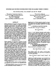
In Figure 4, we examine the validation of Equation (40), which approximates the variance after spatial prediction and temporal prediction. In the experiment, we let S = {176 × 144, 352 × 288}, T = {30f ps}, and R = {r1 }. For ease of presentation, we assume that if the streams have the same spatial resolution, they also have the same QP value. As shown in the bottom row of Figure 4, when the quantization step of the spatial predicting stream is large, ((176 × 144, 30f ps, r1 ) in this case), the propagated distortion dominates the variance calculation, and our rate distortion modeling is very accurate. In contrast, when the quantization step of the spatial predicting stream is small, the constant term or the temporally propagated distortion may dominate the variance, as shown in the top row of Figure 4, and our approximation results are satisfactory. However, if none of the three terms in Equation (40) dominates the process, our modeling is less accurate, as shown in the middle row of Figure 4. In Figure 5, we examine the validation of Equation (41), which approximates the variance of a frame after quality prediction and temporal prediction. In the experiment, we let S = {352 × 288}, T = {30f ps}, and R = {r1 , r2 } (corresponding to using two quality layers). Again, for ease of presentation, we assume that if the streams have the same quality resolution, they also have the same QP value. The results depicted in the bottom row of Figure 5 show that when the quantization step of the quality predicting stream is large ((352 × 288, 30f ps, r1 ) in the case), the propagated distortion dominates the variance calculation, and the rate distortion curves can be well approximated. However, when the quantization step of the quality predicting stream becomes small, the constant term or the temporally propagated distortion may dominate the variance, as shown in the top row of Figure 5. If none of the terms in Equation (41) dominates the process, our variance calculation model becomes less accurate, as shown in the middle row of Figure 5. The results in Figures 3, 4, and 5 show that when the distortion of the dominating term is not significantly larger than that of the other terms, the variances are not well approximated by (39), (40), and (41). A precise distortion model could be obtained by setting all the values of h as 1; however, the analysis of the error propagation for such a model would be overwhelmingly complex. Deriving a more precise variance model whose error propagation can be analyzed easily would be an interesting topic for future research.

C. Performance comparison In this subsection, we compare the coding efficiency of different QP selection schemes. We denote our bit allocation method (discussed in Section VI-B) as Proposed, and compare its performance with that of the state-of-the-art Lagrangianbased method (denoted as Lagrangian) proposed in [8], [7]. The latter uses the weighting of each stream to indicate the importance of the resolution in deriving the optimal bit-allocation; however, the authors do not explain how the weighting values are selected. The Lagrangian method selects the QP values by minimiz-

ing J=

∑ s∈S,t∈T,r∈R

t ∑ w[s,t,r] {

∑

nu(l)

Ji,(s,l,r) },

(77)

l=0 i=nu(l−1)+1

in which w[s,t,r] is the weighting of the resolution [s, t, r]. Here, Ji,(s,l,r) denotes the objective function of the frame i in the stream (s, l, r). It is formulated as follows: Ji,(s,l,r) = (SSD)i,(s,l,r) + λi,(s,l,r) bi,(s,l,r) ,

(78)

where SSD denotes the sum of the squared differences. According to the analysis in [15], if we assign the same QP values (denoted by QP(s,l,r) ) to all the frames in the stream (s, l, r), the value of λ in Equation (78) will be 0.85 × 2(QP(s,l,r) −12)/3 . In our comparison, we let w[s,t,r] be µ[s,t,r] because both of them are supposed to indicate the importance of the resolution in the bit-allocation process. Thus, we compare the optimization with the following objective function: J=

∑ s∈S,t∈T,r∈R

t ∑ µ[s,t,r] {

∑

nu(l)

Ji,(s,l,r) }.

(79)

l=0 i=nu(l−1)+1

In the following experiments, we measure the performance by averaging the coding gain of Proposed over Lagrangian on four sequences: Foreman, News, Dancer and Coastguard. First, we compare the user preference profiles assigned to different temporal resolutions. We let S = {88 × 72}, T = {7.5f ps, 15f ps, 30f ps}, and R = {r1 }. Various values are given to the three preferences, µ[88×72,7.5f ps,r1 ] , µ[88×72,15f ps,r1 ] , and µ[88×76,30f ps,r1 ] so that their sum is equal to 1. We conduct experiments on three rate constraints, namely, 40kbps, 60kbps and 80kbps (corresponding to C in Equation (61)). The average PSNR gain of Proposed over Lagrangian is shown in Figure 6. In addition, as shown in Figure 7, we conduct experiments with the same settings as Figure 6, except that the spatial resolution S = {352×288} and the rate constraints are 80kbps, 120kbps, and 160kbps. From Figures 6 and 7, we observe that Proposed outperforms Lagrangian. The average PSNR gain of Proposed over Lagrangian for temporal scalability is 0.25db in Figure 6 and 0.06db in Figure 7. Next, we compare the rate allocation schemes in terms of different spatial resolutions. In the experiment, we let S = {88×72, 176×144, 352×288}, T = {7.5f ps, 15f ps, 30f ps}, and R = {r1 }. Various values are given to µ[88×72,30f ps,r1 ] , µ[176×144,30f ps,r1 ] , and µ[352×288,30f ps,r1 ] so that their sum is equal to 1. The average PSNR gain of Proposed over Lagrangian is shown in Figure 8. In addition, as shown in Figure 9, we conduct the experiments with the same settings as Figure 8, except that the spatial resolution S = {176 × 144, 352 × 288, 704 × 576}, and the rate constraints become 320kbps, 640kbps, and 1280kbps. For all user preference distributions, the average PSNR gain of Proposed over Lagrangian is 1.38db in Figure 8 and 0.79db in Figure 9. The coding gains in Figures 8 and 9 are much larger than those in Figures 6 and 7. Thus, under our method, the coding gain for spatial scalability is higher than that for temporal scalability. From Figures 8 and 9, we observe that the coding

12

gain depends on the distribution of the user preferences. If most users prefer a lower spatial resolution, the coding gain may be larger than 8db; conversely, if most users prefer a higher spatial resolution, the coding gain may be less than 0.5db. We also compare the rate allocation schemes in terms of different quality resolutions. We let S = {88 × 72}, T = {7.5f ps, 15f ps, 30f ps}, and R = {r1 , r2 , r3 } (three quality layers); and assign various values to µ[88×72,30f ps,r1 ] , µ[88×72,30f ps,r2 ] , and µ[88×72,30f ps,r3 ] so that the sum of their preferences is equal to 1. The average PSNR gain of Proposed over Lagrangian is shown in Figure 10. In addition, as shown in Figure 11, we conduct experiments with the same settings as Figure 10, except that the spatial resolution S = {352 × 288} and the rate constraints are 80kbps, 120kbps, and 160kbps. For all user preference distributions, the average PSNR gain of Proposed over Lagrangian is 0.2db in Figure 10 and 0.05db in Figure 11. Finally, we consider the complexity of the three coding schemes. As shown in Figure 2, motion estimation and mode selection, which are the most time consuming parts of the encoding process in different coding schemes, are only performed once for each macroblock in a GOP. The optimal bitallocation process of all the coding schemes has the same computational complexity order O(MN ), where M represents the number of streams and N denotes the possible QP values for each stream. If the modes and motion vectors are given, motion compensation and quantization can be executed efficiently in all the schemes. In our experiments, at a high coding rate, the computation time of the Proposed method is about 3 times longer than that of the JSVM encoder; however, at a low coding rate, it is only 1.5 times longer. VIII. C ONCLUSION We present a theoretical analysis of joint R-D optimization for mult-layer coding. The data dependency structure of temporal, spatial, and quality prediction is fully explored in the analysis. In addition, we demonstrate the importance of the end user’s preference to the coding performance of SVC. We derive that the average PSNR of SVC is the weighted average of the bit rates assigned to individual streams. The weighting factor is a function of all the affected layers and their corresponding preference factors. We also propose an optimal bit allocation algorithm that controls the encoder rate with subscribers’ preference information. Comparison of the algorithm’s performance with that of a state-of-the-art coder shows that it achieves a significant PSNR gain over the compared method. In a future work, we will extend our analysis to study the joint source and channel coding problem under SVC.

ACKNOWLEDGMENTS The authors wish to thank the reviewers and the associate editor for their insightful comments, which have helped us improve the quality of the paper significantly.

Table 1. The proposed optimal bit allocation algorithm with known preference information (1) Let QPi = 51 for each stream and let F = {}. (2) Run SVC to obtain the actual number of bits used in the current QP assignment. (3) Derive the values of h, κ, and γ from QP , and compute the weight wi . (4) Based on the weight, assign a stream to either Sλ>0 or Sλ=0 . (5) If all the streams are in F , the algorithm stops. Otherwise, for a stream i not in F , there are two possibilities: i ∈ Sλ>0 or i ∈ Sλ=0 . (6) Case Sλ>0 : (6.1) Let wi = maxk∈Sλ>0 ,k∈F / wk ; that is, the coding error of the stream i has the largest weight. If QPi = 1, the stream has the largest bit assignment and it is added to F . Otherwise, increase the number of bits assigned to the stream by reducing its QP value; QPi = max{QPi − 1, 1}. (6.2) Run SVC to obtain the actual number of bits for the new value of QP . If bi > Bi , let QPi = QPi + 1, add stream i to F , and go to step 5; otherwise, go to step 3. (7) Case Sλ=0 : ∑ (7.1) Reduce QPi until bi >

C− ∑

k∈Sλ>0 k∈Sλ=0

Bk

wk

wi ,

or bi > Bi , or QPi = 0. Then, add i to F and let QPi = QPi + 1; and go to step 3. Appendix 1: Variance approximation In this appendix, we provide a simple example to illustrate how the dependency of frames in video coding can affect the rate-distortion analysis significantly. In the following, the texture means the residual obtained after predicting a frame. We consider two cases and use three frames (frames 1, 2, and 3) to demonstrate the benefits derived by re-writing Equation (24) as Equation (25). Case 1: Independent rate distortion curves Assuming the three frames are encoded separately with the variances of the texture σ12 , σ22 , σ22 and the model coefficients γ1 and γ2 and γ3 respectively (according to Equation (3)), the optimal rate allocation problem involves minimizing the following equation:

=

σ12

D1 (b1 )D2 (b2 )D3 (b3 ) 2 exp (−γ1 b1 )σ2 exp (−γ2 b2 )σ32 exp (−γ3 b3 ) = σ12 σ22 σ32 exp (−(γ1 b1 + γ2 b2 + γ3 b3 )).

(80a) (80b)

Thus, after taking the logarithm on both sides of the equation, we obtain the linear relationship between the log-distortion and the bit rate allocated to each frame. As a result, the optimal rate allocation solution can be derived efficiently by using linear programming methods. Case 2: Dependent rate distortion curves In this case, we show how the dependency affects the rate allocation results based on the ρ-domain source model. We assume that frame 2 is temporally predicted by frame 1 and

13

frame 3. Because the texture of frame 2 is dependent on the reconstructed referred (predicting) frames in the prediction steps, σ22 should be a function of the rates allocated to frame 1 and frame 3. The optimal rate allocation problem involves minimizing the following equation:

that adjust the variance of the respective dominating terms to the actual variance. Depending on which term in h is the dominating term, the distortion in Equation (84) becomes either

D1 (b1 )D2 (b1 , b2 , b3 )D3 (b3 ) = σ12 exp (−γ1 b1 )σ22 (b1 , b3 ) exp (−γ2 b2 )σ32 exp (−γ3 b3 ) (81a) = σ12 σ22 (b1 , b3 )σ32 exp (−(γ1 b1 + γ2 b2 + γ3 b3 )), (81b)

D1 (b1 )D2 (b1 , b2 , b3 )D3 (b3 ) = κ1 σ12 σ32 var(C2 ),

(86)

D1 (b1 )D2 (b1 , b2 , b3 )D3 (b3 ) = κ2 σ12 σ32 A(b1 , b2 , b3 ),

(87)

or

where σ22 (b1 , b3 ) implies that the variance of frame 2 is dependent on the rates b1 and b3 . The detailed derivation of the effects of b1 and b3 on σ22 is given in Appendix 2. Using the result of Appendix 2, we have ( ) var(C2 ) 2 T σ2 (b1 , b3 ) = h2 , (82) 1 {C1α C3β D1 (b1 )D3 (b3 )} 2

where A(b1 , b2 , b3 ) is given in Equation (85). Thus, our approach can preserve the simple linear relationship between the log-distortion and the allocated bit rates of dependent frames. Using a simpler R-D analysis of distortion propagation from referred frames/layers to referring frames/layers makes the optimal rate allocation process much more straightforward.

where var(C2 ), C1α , and C3α are constants, and D1 (b1 ) and D3 (b3 ) represent the distortion of frame 1 and frame 3 respectively. Let h12 and h22 be the first and second components of column vector h2 . Equation (82) can be written as

Appendix 2: The two-stream relation of temporal prediction at a low bit rate

σ22 (b1 , b3 )

=

1 h12 var(C2 ) + h22 {C1α C3β D1 (b1 )D3 (b3 )} 2 .

(83)

The ρ-domain source model is used for the distortions D1 (b1 ) and D3 (b3 ) in Equation (83). We obtain =

D1 (b1 )D2 (b1 , b2 , b3 )D3 (b3 ) 2 2 1 σ1 σ3 (h2 var(C2 ) + h22 A(b1 , b2 , b3 )),

(84)

where A(b1 , b2 , b3 ) = {C1α C3β σ12 1 2

exp (−γ1 b1 )σ32

exp (−γ3 b3 )} exp (−(γ1 b1 + γ2 b2 + γ3 b3 )).

(85)

Note that, in Equation (84), the two leading terms begin with h12 and h22 respectively. Thus, we cannot obtain the simple linear relationship between the log-distortion and the rates allocated to frames by taking the logarithm on both sides of the equation. This example shows that the complexity of optimal rate-allocation analysis of the three dependent frames can increase. If more frames are involved, the distortion may be comprised of several terms; hence, the rate-allocation analysis would be even more complicated. Moreover, if we consider spatial, temporal, and quality dependency simultaneously, as in H.264/SVC, the optimal rate allocation problem would become overwhelmingly complicated and impossible to solve efficiently. The above analysis explains why we only allow the vector h in Equations (39),(40), and (41) to have one nonzero component (i.e., dominating component). As a result, the variance of each predicted frame is comprised of only one term, so we can maintain the simple linear relationship between the log-distortion and the bit rate in the analysis. In our example, σ22 is approximated as either κ1 var(C2 ) or 1 κ2 {C1α C3β σ12 exp (−γ1 b1 )σ32 exp (−γ3 b3 )} 2 , not as a linear combination of them, where κ1 and κ2 are scaling factors

The two-stream relation explores the data-dependency between the predicting and predicted stream in SVC. We now derive the distortion between the two streams due to temporal prediction at a low bit rate. In the following analysis, the pixels of a frame are arranged as a vector. For temporal prediction at a low bit rate, Equation (15) can be approximated as (∆i,(0,l) )1,t = Pi,i−m ∆i−m,(0,l−1,1) + Pi,i+m ∆i+m,(0,l−1,1) , (88) where Pi,i−m and Pi,i+m are the matrices of the motion vectors. Without loss of generality, we assume that a pixel in (∆i,(0,l) )1,t is estimated by a linear combination of one pixel in ∆i−m,(0,l−1,1) and one pixel in ∆i+m,(0,l−1,1) . Thus, the p-th pixel in (∆i,(0,l) )1,t can be written as (∆i,(0,l) )1,t (p) = a∆i−m,(0,l−1,1) (f1 (p))+b∆i+m,(0,l−1,1) (f2 (p)), (89) where a and b are the prediction weights of ∆i−m,(0,l−1,1) and ∆i+m,(0,t−1,1) respectively; and f1 (p) and f2 (p) are the corresponding pixels in the predicting residuals. As usual, the pixels can be derived from the motion vectors. Because motion estimation finds the most similar blocks in the predicting residual in order to estimate the target block, we can assume that there are several pairs of pixels in which ∆i−m,(s,t−1,1) (f1 (p)) and ∆i+m,(0,t−1,1) (f2 (p)) have similar values; that is, for several pairs of (f1 (p), f2 (p)), ∆i−m,(0,l−1,1) (f1 (p)) ≈ ∆i+m,(0,l−1,1) (f2 (p)).

(90)

Substituting the above result into Equation (89), we have ((∆i,(0,l) )1,t )2 ≈ (a + b)2 (∆i−m,(0,l−1,1) (f1 (p)))2 .

(91)

Let N 2 denote the number of pixels in (∆i,(0,l) )1,t . If the

14

interpolation kernel is used, then a + b = 1, and we have N 1 ∑ ((∆i,(0,l) )1,t (p))2 N 2 p=1 2

2 σi,(0,l,1)

=

N ∑ (C α )1,t i−m,(0,l−1)

(92)

2

≈

=

N2

2

(∆i−m,(0,l−1,1) (f1 (p)))

p=1

(93) (94)

(C α )1,t i−m,(0,l−1) Di−m,(0,l−1,1) ,

prediction method. As shown in Equation (29), at a low bit rate and var(U (∆i,(s−1,l,1) )) > var(Pi,i−m ∆i−m,(s,l−1,1) + Pi,i+m ∆i+m,(s,l−1,1) ), the residual ∆1,s i,(s,l) (p) can be approximated as T ∆1,s i,(s,l) (p) ≈ U (vec(∆i,(s−1,l,1) [p])),

where T is the transpose operation. Taking the square of ∆1,s i,(s,l) (p), we can derive that 2 (∆1,s i,(s,l) (p))

where (C α )1,t i−m,(0,l−1) is related to the proportion of the pixels used to perform forward prediction in ∆i−m,(0,l−1,r) : ∑N 2 2 p=1 (∆i−m,(0,l−1,1) (f1 (p))) . (95) ∑N 2 2 p=1 (∆i−m,(0,l−1,1) (p)) 1,t The value of (C α )i−m,(0,l−1) depends on the motion vectors. It becomes a constant after the motion vectors have been obtained. For the frames of slow motion objects, almost all the pixels in ∆i−m,(0,l−1,r) will be used in the prediction process; thus, (C α )1,t i−m,(0,l−1) ≈ 1. In a similar way, we can derive that 2 σi,(0,l,1)

≈

(C β )1,t i+m,(0,l−1) Di+m,(0,l−1,1) ,

(96)

∑N 2

2 p=1 (∆i+m,(0,l−1,1) (f2 (p))) . ∑N 2 2 p=1 (∆i+m,(0,l−1,1) (p))

= trace(U U T (vec(∆i,(s−1,l,1) [p])) (vec(∆i,(s−1,l,1) [p]))T )

(97)

(C β )1,t i+m,(0,l−1) is a constant after the motion vectors have been obtained. For frames that contain slow motion objects, (C β )1,t i+m,(0,l−1) ≈ 1. Combining Equations (94) and (96), we have 2 σi,(0,l,1) ≈ β 1,t (C α )1,t i−m,(0,l−1) (C )i+m,(0,l−1)

(100)

≤ trace(U U )trace((vec(∆i,(s−1,l,1) [p])) T

(vec(∆i,(s−1,l,1) [p]))T )

(101)

T

= trace(U U )∥vec(∆i,(s−1,l,1) [p])∥F(102) ≤ ∥U ∥22 ∥vec(∆i,(s−1,l,1) [p])∥F .

(103)

Equations (101), (102), and (103) are derived by using the properties of the Frobenius norm: ∥AB∥2F ≤ ∥A∥2F ∥B∥2F , and ∥A∥2F = trace(AT A), (104) for any real matrices A and B. If U represents an interpolation, then ∥U ∥22 ≤ ∥U ∥21 = 1. As a result, Equation (103) becomes 2 (∆1,s i,(s,l) (p)) ≤ ∥vec(∆i,(s−1,l,1) [p])∥F .

1,t where (C β )i+m,(0,l−1) is calculated as follows:

(99)

(105)

Let |U | denote the size of the vector U . Because any pixel in ∆i,(s−1,l,1) is used at most |U | times in the spatial prediction process, the variance of ∆1,s i,(s−1,l) can be calculated as =

4N 1 ∑ 1,s (∆ (p))2 4N 2 p=1 i,(s−1,l)

≤

4N 1 ∑ ∥vec(∆i,(s−1,l,1) [p])∥2F (107) 4N 2 p=1

2

2 σi,(s,l,1)

(106)

2

|U | (108) ∥vec(∆i,(s−1,l,1) )∥2F 4N 2 |U | = Di,(s−1,l,1) . (109) 4 Equation (109) gives the distortion between two corresponding frames in the spatial prediction process. If bilinear interpolation is used, (i.e., 4 pixels are involved in the interpolation), we have |U | = 4. Then, we can introduce a constant (C ω )1,s i,(s−1,l) and re-write Equation (109) as follows: ≤

1 2

Di−m,(0,l−1,r) Di+m,(0,l−1,r) ) , (98) which is the geometric mean of the results of Equations (94) and (96). Appendix 3: The two-stream relation of spatial residual prediction at a low bit rate In the following, we derive the relation between the distortion of two frames during inter-layer spatial prediction at a low bit rate. Let the size of a frame in spatial layer s − 1 be N 2 . Without loss of generality, we assume a dyadic spatial scalability structure, where the number of pixels of a frame in spatial layer identifier s is four times greater than that of the corresponding frame in spatial layer identifer s − 1. r,s Let ∆r,s i,(s,l) (p) denote the p-th pixel in ∆i,(s,l) , and let ∆i,(s−1,l,1) [p] denote the pixels in ∆i,(s−1,l,1) involved in the spatial prediction of pixel ∆r,s i,(s,l) (p). We use the vec operator to change the pixels in the block ∆si,(s−1,l,1) [p] into a column vector U , and use the latter to represent the spatial

2 σi,(s,l,1) = (C ω )1,s i,(s−1,l) Di,(s−1,l,1) .

(110)

Appendix 4: The two-stream relation of quality residual prediction at a low bit rate In the following, we derive the relation between the distortion of two frames during inter-layer quality prediction at a low bit rate. Let the size of a frame in spatial layer s be r,q N 2 . Let ∆r,q i,(s,l) (p) denote the p-th pixel in ∆i,(s,l) , and let ∆i,(s,l,r−1) [p] denote the pixels in ∆i,(s,l,r−1) involved in the quality prediction of pixel ∆r,q i,(s,l) (p). We use the vec

15

operator to change the pixels in the block ∆si,(s,l,r−1) [p] into a column vector Y , and use the latter to represent the quality prediction method. As shown in Equation (29), at a low bit rate and var(Y (∆i,(s,l,r−1) )) > var(Pi,i−m ∆i−m,(s,l−1,r) + Pi,i+m ∆i+m,(s,l−1,r) ), the residual ∆r,q i,(s,l) (p) can be approximated as T ∆r,q i,(s,l) (p) ≈ Y (vec(∆i,(s,l,r−1) [p])),

(111)

where T is the transpose operation. Taking the square of ∆r,q i,(s,l) (p), we can derive that 2 (∆r,q i,(s,l) (p))

= trace(Y Y T (vec(∆i,(s,l,r−1) [p])) (vec(∆i,(s,l,r−1) [p]))T )

(112)

≤ trace(Y T Y )trace((vec(∆i,(s,l,r−1) [p])) (vec(∆i,(s,l,r−1) [p]))T )

(113)

T

= trace(Y Y )∥vec(∆i,(s,l,r−1) [p])∥F(114) ≤

∥Y ∥22 ∥vec(∆i,(s,l,r−1) [p])∥F .

(115)

Equations (113), (114), and (115) are derived by using the properties of the Frobenius norm: ∥AB∥2F ≤ ∥A∥2F ∥B∥2F , and ∥A∥2F = trace(AT A), (116) for any real matrices A and B. Because Y represents selection of pixels, we have ∥Y ∥22 ≤ 1. As a result, Equation (115) becomes 2 (∆r,q i,(s,l) (p)) ≤ ∥vec(∆i,(s,l,r−1) [p])∥F .

(117)

The variance of ∆r,q i,(s,l) can be calculated as =

N 1 ∑ r,q (∆ (p))2 N 2 p=1 i,(s,l)

≤

N 1 ∑ ∥Y ∥22 ∥vec(∆i,(s,l,r−1) [p])∥2F(119) N 2 p=1

2

2 σi,(s,l,r)

[4] H. Schwarz, D. Marpe, and T. Wiegand, “Overview of the scalable video coding extension of the H.264/AVC standard,” IEEE Transactions on Circuits and Systems for Video Technology, vol. 17, no. 9, pp. 1103– 1120, 2007. [5] M. Wien, H. Schwarz, and T. Oelbaum, “Performance analysis of SVC,” IEEE Transactions on Circuits and Systems for Video Technology, vol. 17, no. 12, pp. 1771–1771, 2007. [6] G. J. Sullivan and T. Wiegand, “Rate-distortion optimization for video compression,” IEEE Signal Processing Magazine, vol. 15, no. 6, pp. 74–90, November 1998. [7] K. Ramchandran, A. Ortega, and M. Vetterli, “Bit allocation for dependent quantization with applications to multiresolution and MPEG video coders,” IEEE Transactions on Image Processing, vol. 3, no. 5, pp. 533– 545, 1994. [8] H. Schwarz and T. Wiegand, “R-D optimized multi-layer encoder control for SVC,” in IEEE International Conference on Image Processing, Sepetember 2007, pp. 281–284. [9] M. Koziri and A. Eleftheriadis, “Joint quantizer optimization for scalable coding,” in IEEE International Conference on Image Processing, October 2010. [10] J. Reichel, H. Schwarz, and M. Wien, “Joint Scalable Video Model 11 (jsvm 11),” Joint Video Team, Doc, JVT-X202, July 2007. [11] Z. He and S. K. Mitra, “Optimum bit allocation and accurate rate control for video coding via rho domain source modeling,” IEEE Transactions on Circuits and Systems for Video Technology, vol. 12, no. 10, pp. 840– 849, 2002. [12] Q. Zhang, Q. Guo, Q. Ni, W. Zhu, and Y.-Q. Zhang, “Sender-adaptive and receiver driven layered multicast for scalable video over the internet,” IEEE Transactions on Circuits and Systems for Video Technology, vol. 15, no. 4, pp. 482–495, April 2005. [13] H. Li, Z. Li, and C. Wen, “Fast mode decision algorithm for inter-frame coding in fully scalable video coding,” IEEE Transactions on Circuits and Systems for Video Technology, vol. 16, no. 7, pp. 889 –895, july 2006. [14] L. Czúni, G. Császár, and A. Licsár, “Estimating the optimal quantization parameter in H.264,” in IEEE International Conference on Pattern Recognition, August 2006, pp. 330–333. [15] T. Wiegrand, H. Schwarz, A. Joch, F.Kossentini, and G. J. Sullivan, “Rate-constrained coder control and comparison of video coding standards,” IEEE Transactions on Circuits and Systems for Video Technology, vol. 13, no. 7, July 2003.

(118)

2

1 ∥vec(∆i,(s,l,r−1) )∥2F N2 = Di,(s,l,r−1) .

≤

(120) (121)

Equation (121) gives the distortion between two corresponding frames in the quality prediction process. Then, we can introduce a constant (C ω )r−1,q i,(s,l) and re-write Equation (121) as follows: 2 σi,(s,l,r) = (C ω )r−1,q i,(s,l) Di,(s,l,r−1) .

(122)

R EFERENCES [1] P. Steenkiste, “Adaptation models for network-aware disributed computation,” in Workshop on Communication, Architecture, and Applicatios for Network-based Parallel Computing, January 1999, pp. 16–31. [2] B. Tierney, D. Gunter, J. Lee, M. Stoufer, and J. B. Evans, “Enabling network-aware applications,” in IEEE International Symposium on High Performance Distributed Computing, 2001, pp. 281–288. [3] T. Wiegand, G. J. Sullivan, G. Bjontegaaard, and A. Luthra, “Overview of the H.264/AVC video coding standard,” IEEE Transactions on Circuits and Systems for Video Technology, vol. 13, no. 7, pp. 560–576, July 2003.

Fig. 1. The data dependency structure for coarse-grain quality prediction of H.264/SVC.

16

Foreman QP(176×144,30fps,r ) =26

Dancer QP(176×144,30fps,r ) =26

1

60

News QP(176×144,30fps,r ) =26

1

50

Average MSE Approximation

50

1

200


40


150

30

30

MSE

MSE

MSE

40 100

20 20 50

10

10 0 0

500 1000 1500 2000 Rate b(352×288,30fps,r ) (kbits/s)

0 0

2500

500 1000 Rate b(352×288,30fps,r

1

0 0

2000

3000 (kbits/s)

)

4000

1

News QP(176×144,30fps,r ) =38

100

1

300



250

80

80

200

60

MSE

60

MSE

MSE

1000 2000 Rate b(352×288,30fps,r

1


100

1500 (kbits/s)

Dancer QP(176×144,30fps,r ) =38

1

120

)

1


150

40 40

100 20

20 0 0

1000 2000 Rate b(352×288,30fps,r

)

3000 (kbits/s)

50

0 0

4000


1

1000 2000 Rate b(352×288,30fps,r

1

Foreman QP(176×144,30fps,r ) =50 200


3000 (kbits/s)

4000

News QP(176×144,30fps,r ) =50

1

200

)

1

Dancer QP(176×144,30fps,r ) =50

1

250

0 0

2500

1

300



250

150 MSE

150

MSE

MSE

200 100

150

100 100 50

50

50

0 0

1000 2000 Rate b(352×288,30fps,r

)

3000 (kbits/s)

0 0

4000

500 1000 1500 2000 2500 Rate b(352×288,30fps,r ) (kbits/s)

1

0 0

3000


16 Average MSE Approximation

12 MSE

MSE

MSE

8

4

10 8 6

3

4

4

2 500

1000 1500 Rate b(352×288,30fps,r ) (kbits/s)

2 500

2000

1000 1500 Rate b(352×288,30fps,r ) (kbits/s)

2

40

MSE

30

20 0 0

50 100 Rate b(352×288,7.5fps,r

)

150 (kbits/s)

0 0

200

)

150 (kbits/s)

0 0

200

200

MSE


100 200 300 400 500 Rate b(352×288,7.5fps,r ) (kbits/s)

600

140

100

250

80

200

60


80

200

60

150

40

100

20

50


0 0

1000 2000 Rate b(352×288,30fps,r

)

3000 (kbits/s)

50

0 0

4000

500 1000 1500 2000 2500 Rate b(352×288,30fps,r ) (kbits/s)

600 (kbits/s)

0 0

800

0 0

400

30

)

1

1500 (kbits/s)

2000

0 0

Fig. 5. Approximation of the distortion of the predicted layer due to quality prediction and temporal prediction based on Equation (41). The prediction accuracy depends on the QP values of the predicting layer.


250

Average PSNR Gain: 40kbps 150 100 50

10 500 1000 Rate b(352×288,7.5fps,r

4000

200

40

20

20

3000 (kbits/s)

1

300

MSE

MSE

40

1500

)

2

1

50

60

500 1000 Rate b(352×288,7.5fps,r ) (kbits/s)

1000 2000 Rate b(352×288,30fps,r

News QP(352×288,7.5fps,r ) =50


60

80 MSE

300 (kbits/s)

1

70 Average MSE Approximation

100

)

1

Dancer QP(352×288,7.5fps,r ) =50

1

120

0 0

100 200 Rate b(352×288,7.5fps,r

0 0

3000

2

200 400 600 800 Rate b(352×288,7.5fps,r ) (kbits/s) 1

1000

0 0

500 1000 1500 2000 2500 Rate b(352×288,7.5fps,r ) (kbits/s) 1

Fig. 3. Approximation of the distortion of the predicted layer due to temporal prediction based on Equation (39). The prediction accuracy depends on the QP values of the predicting layer.

3000

Average PSNR Gain: 60kbps

1.5 1 0.5 0 1

0.5

µ[88x76,15fps,r

0 0 ]

1

1 0.5 µ[88x76,7.5fps,r ] 1

Average PSNR Gain (db)

)

1

150 100

20


200 400 Rate b(352×288,7.5fps,r

Foreman QP(352×288,7.5fps,r ) =50


300

100

40

50

1

250

MSE

MSE

MSE

0 0

350

1

40 20

4000

1


120

3000 (kbits/s)

)

2

News QP(352×288,30fps,r ) =50

1

2

60

1000 2000 Rate b(352×288,30fps,r

Dancer QP(352×288,30fps,r ) =50


100 80

0 0

2500

2

150

News QP(352×288,7.5fps,r ) =38

1

100


120

50 100 Rate b(352×288,7.5fps,r

3000

1

60

Dancer QP(352×288,7.5fps,r ) =38

1

140

500 1000 1500 2000 2500 Rate b(352×288,30fps,r ) (kbits/s) Foreman QP(352×288,30fps,r ) =50

1

1

Foreman QP(352×288,7.5fps,r ) =38

60 40

0 0

2

20

10

80

20

0 0

40

20

20


1.5 1 0.5 0 1

0.5

µ[88x76,15fps,r

0 0 ]

1

1 0.5 µ[88x76,7.5fps,r ] 1


MSE

MSE

40

100

10

80

40


120

10


100

50 60

20

MSE

80

140


MSE


60

30

1

120

MSE


40

MSE

MSE News QP(352×288,7.5fps,r ) =26

1

1

30

50

3500

2

News QP(352×288,30fps,r ) =38

1


60


Dancer QP(352×288,30fps,r ) =38

1

70

2 1000

2000

2


Dancer QP(352×288,7.5fps,r ) =26


14

6

70

4000

1

1

6


12 10

1

3000 (kbits/s)

News QP(352×288,30fps,r ) =26

Dancer QP(352×288,30fps,r ) =26

1

14

5

Foreman QP(352×288,7.5fps,r ) =26

)

1

Fig. 4. Approximation of the distortion of the predicted layer due to spatial prediction and temporal prediction based on Equation (40). The prediction accuracy depends on the QP values of the predicting layer.

Fig. 2. The proposed encoding structure supports the combined scalability. In our implementation, motion estimation and mode selection are based on JSVM 9.18. Each layer performs its own motion estimation and mode selection. Note that if the inter-layer QP selection step is removed, then the coding structure is exactly the same as that of H.264/SVC. M QP is defined as the QP values used to derive the modes and the motion vectors of macroblocks. The model parameters for Inter-Layer QP Selection are h, κ, and γ. They are updated in each iteration of our optimal bit allocation algorithm.

100

1000 2000 Rate b(352×288,30fps,r

1

1.5 1 0.5 0 1

0.5

µ[88x76,15fps,r

0 0 ]

1

1 0.5 µ[88x76,7.5fps,r ] 1

Fig. 6. The PSNR gain of Proposed over Lagrangian in terms of temporal scalability. The preferences µ[88×72,7.5f ps,r1 ] and µ[88×72,15f ps,r1 ] are shown; and, the preference µ[88×72,30f ps,r1 ] can be obtained by (1 − µ[88×72,7.5f ps,r1 ] − µ[88×72,15f ps,r1 ] ).

17

0

−1 1

0.5

1 0.5 µ[352x288,7.5fps,r

0 0

µ[352x288,15fps,r

]

1

0.2

0.1

0 1

0.5

µ[352x288,15fps,r

]

0 0 ]

1

1

Average PSNR Gain: 160kbps Average PSNR Gain (db)



Average PSNR Gain: 80kbps 1

1 0.5 µ[352x288,7.5fps,r

]

1

1

0.5

0 1

0.5

0 0

µ[352x288,15fps,r

]

1

1 0.5 µ[352x288,7.5fps,r

]

1

Fig. 7. The PSNR gain of Proposed over Lagrangian in terms of temporal scalability. The preferences µ[352×288,7.5f ps,r1 ] and µ[352×288,15f ps,r1 ] are shown; and, the preference µ[352×288,30f ps,r1 ] can be obtained by (1 − µ[352×288,7.5f ps,r1 ] − µ[352×288,15f ps,r1 ] ).

1 0 1

0.5

0 0

µ[176x144,30fps,r

]

1

1 0.5 µ[88x76,30fps,r ] 1



2




10

5

0 1

0.5

0 0

µ[176x144,30fps,r

]

1

1 0.5 µ[88x76,30fps,r ]

10

5

0 1

0.5

µ[176x144,30fps,r

0 0 ]

1

1

1 0.5 µ[88x76,30fps,r ] 1

Fig. 8. The PSNR gain of Proposed over Lagrangian in terms of spatial scalability. The preferences µ[88×72,30f ps,r1 ] and µ[176×144,30f ps,r1 ] are shown; and, the preference µ[352×288,30f ps,r1 ] can be computed by (1 − µ[88×72,30f ps,r1 ] − µ[176×144,30f ps,r1 ] ).

1 0 1

0.5

0 0 ]

1

1 0.5 µ[176x144,30fps,r

4

2

0 1

0.5

0 0

µ[352x288,30fps,r

]

]

1

1


2

µ[352x288,30fps,r





1 0.5 µ[176x144,30fps,r

10

5

0 1

0.5

µ[352x288,30fps,r

]

0 0 ]

1

1

1 0.5 µ[176x144,30fps,r

]

1

Fig. 9. The PSNR gain of Proposed over Lagrangian in terms of spatial scalability. The preferences µ[176×144,30f ps,r1 ] and µ[352×288,30f ps,r1 ] are shown; and, the preference µ[704×576,30f ps,r1 ] can be computed by (1 − µ[176×144,30f ps,r1 ] − µ[352×288,30f ps,r1 ] ).

0.2

0 1

0.5

µ[88x76,30fps,r

0 0 ]

2

1 0.5 µ[88x76,30fps,r ] 1




Average PSNR Gain: 40kbps 0.4

1

0.5

0 1

0.5

0 0

µ[88x76,30fps,r

]

2

1 0.5 µ[88x76,30fps,r ]

1.5 1 0.5 0 1

0.5

µ[88x76,30fps,r

0 0 ]

2

1

1 0.5 µ[88x76,30fps,r ] 1

Fig. 10. The PSNR gain of Proposed over Lagrangian in terms of quality scalability. The preferences µ[88×72,30f ps,r1 ] and µ[88×72,30f ps,r2 ] are shown; and, the preference µ[88×72,30f ps,r3 ] can be computed by (1 − µ[88×72,30f ps,r2 ] − µ[88×72,30f ps,r3 ] ).



0.005

0 1

0.5

µ[352x288,30fps,r

0 0 ]

2

1 0.5 µ[352x288,30fps,r

]

1



Average PSNR Gain: 160kbps 0.01

0.2

0.1

0 1

0.5

µ[352x288,30fps,r

0 0 ]

2

1 0.5 µ[352x288,30fps,r

]

1

0.1

0.05

0 1

0.5

µ[352x288,30fps,r

0 0 ]

2

1 0.5 µ[352x288,30fps,r

Fig. 11. The PSNR gain of Proposed over Lagrangian in terms of quality scalability. The preferences µ[352×288,30f ps,r1 ] and µ[352×288,30f ps,r2 ] are shown; and, the preference µ[352×288,30f ps,r3 ] can be computed by (1 − µ[352×288,30f ps,r2 ] − µ[352×288,30f ps,r3 ] ).

]

1

18

Guan-Ju Peng was born in Taiwan in 1982. He received a B.S. degree in Computer Science and Information Engineering, and an M.S. degree in Electrical Engineer from National Taiwan University in 2004 and 2006 respectively. Since 2007, he has been a research assistant in Dr. Wen-Liang Hwangs laboratory at the Institute of Information Science, Academia Sinica. Currently, he is studying for his Ph.D under the direction of Prof. Sao-Jie Chen at the Graduate Institute of Electronic Engineering, National Taiwan University. His research interests include video coding, video transmission, and wavelets.

Wen-Liang Hwang received his B.S. Degree in Nuclear Engineering from National Tsing Hua University, Hsinchu, Taiwan; his M.S. Degree in Electrical Engineering from the Polytechnic Institute of New York, New York; and, in 1993, his Ph.D. in Computer Science from New York University, New York. He was a postdoctoral researcher with the Department of Mathematics, University of California, Irvine in 1994. In January 1995, he became a member of the Institute of Information Science, Academia Sinica, Taipei, Taiwan, where he is currently a Research Fellow. He is co-author of the book: ”Practical TimeFrequency Analysis,” Academic Press, 1998. Currently, Dr. Hwang is an associate editor of the Journal of Wavelet Theory and Applications and International Journal of Wavelets, Multiresolution and Information Processing. His research interests include wavelet analysis, signal and image processing, and multimedia compression and transmission. In 2001, he was awarded the Academia Sinica Research Award for Junior Researchers.

Sao-Jie Chen received the B.S. and M.S. degrees in electrical engineering from the National Taiwan University, Taipei, Taiwan, ROC, in 1977 and 1982 respectively, and the Ph.D. degree in electrical engineering from the Southern Methodist University, Dallas, USA, in 1988. Since 1982, he has been a member of the faculty in the Department of Electrical Engineering, National Taiwan University, where he is currently a full professor. During the fall of 1999, he was a visiting professor in the Department of Computer Science and Engineering, University of California, San Diego, USA. During the fall of 2003, he held an academic visitor position in the Department of System Level Design, IBM Thomas J. Watson Research Center, Yorktown Heights, New York, USA. He obtained the ”Outstanding Electrical Engineering Professor Award” by the Chinese Institute of Electrical Engineering in December 2003 to recognize his excellent contributions to EE education. During the falls of 2004 to 2009, he was a visiting professor in the Department of Electrical and Computer Engineering, University of Wisconsin, Madison, USA. He was also an International Adjunct Professor in the Department of Electrical and Computer Engineering, University of Illinois, Urbana-Champaign, for the Spring Semester, 2010 and 2011. His current research interests include: VLSI physical design, SOC hardware/software co-design, Network-on-Chip, and Wireless LAN and Bluetooth IC design. Dr. Chen is a member of the Chinese Institute of Engineers, the Chinese Institute of Electrical Engineering, the Institute of Taiwanese IC Design, the Association for Computing Machinery, a senior member of the IEEE Circuits and Systems and the IEEE Computer Societies