KINETICS. Jorge Diaz-Salgado* Alexander Schaum* ... cascade temperature linear PI loops are employed, ..... differential equations (ODE's) and 5 algebraic.
8th International IFAC Symposium on Dynamics and Control of Process Systems Preprints Vol.3, June 6-8, 2007, Cancún, Mexico
INTERLACED ESTIMATOR-CONTROL DESIGN FOR CONTINUOUS EXOTHERMIC REACTORS WITH NON-MONOTONIC KINETICS Jorge Diaz-Salgado ∗ Alexander Schaum ∗ Jaime A. Moreno ∗ Jesus Alvarez ∗∗ ∗
Instituto de Ingenier´ıa, Universidad Nacional Aut´ onoma de M´exico (UNAM). Cd. Universitaria, 04510 M´exico D.F. ∗∗ Universidad Autonoma Metropolitana-Iztapalapa Apdo. 55534, (UAM-I), 09340 M´exico DF.
Abstract: The problem of controlling continuous exothermic jacketed reactors with non-monotonic kinetics as well as temperature, level and flow measurements is addressed. The application of a constructive control procedure, with emphasis on the attainment of linearity, decentralization, robustness and model independency features, yields: (i) a control scheme with PI volume and cascade temperature loops, (ii) a material balance concentration controller driven by the integral actions of the temperature controller, and (iii) a closed-loop nonlocal stability criterion coupled with conventional-like tuning guidelines. The approach is tested with a c representative example through simulations. Copyright °2007 IFAC Keywords: Reactor Control, PI Controllers, Constructive Control
1. INTRODUCTION
and the concentration is regulated by adjusting the reactant dosage via supervisory or advisory control. Thus, the objective of a process-control design scheme is to attain a closed-loop operation with an adequate compromise between safety, operability, productivity, and quality in the light of investment operation costs. Hitherto, this problem has been addressed with a diversity of procedures (Smets et al., 2002) that lack systematization and formal closed-loop stability assessments, and recently with an output-feedback nonlinear passive controller (Diaz-Salgado et al , 2006). In spite of its robustness oriented developement, the consideration of the las controller should rise complexity, reliability, maintenance and cost concerns among practitioners because: (i) the scheme is rather complex and model dependent, (ii) the volume and jacket temperature control components are
An important class of chemical and biological materials are produced in continuous reactors with non-monotonic reaction rate (Elnashaie et al., 1990; Lapidus et al., 1977). In exothermic reactors, the interplay between heat generationremoval and non-monotonic kinetics manifests itself as strongly nonlinear behavior, with asymmetric input-output coupling, steady-state (SS) multiplicity, and parametric sensitivity (Aris, 1969). Operation at maximum production rate means lack of local observability about the nominal SS (Diaz-Salgado et al., 2006). To overcome this obstacle for estimator-based control, the reactor can be operated at a reaction rate sufficiently below its maximum value, at the cost of less productivity. In industry (Shinskey, 1988), volume and cascade temperature linear PI loops are employed,
43
The definition of nonlocal stability that underlies our study is stated next. Consider a nonlinear system with time-varying exogenous input de (t):
not included, and (iii) a formal stability assessment is lacking. These considerations motivate the present study. In this work, employing the same robustness oriented approach, the reactor problem is addressed within a constructive control framework. The result is a measurement-driven (MD) control scheme with: (i) decentralized linear PI volume and cascade temperature loops, a ratio-type material-balance concentration controller, (ii) reduced model dependency, especially of the components that perform the stabilization task, and (iii) a nonlocal closed-loop robust stability criterion coupled with conventional-like tuning guidelines. The approach is illustrated with a representative example through simulations.
e˙ = fe (e, de ), e(0) = e0 , fe (0, 0) = 0 The steady-state e = 0 is input-to-state (IS) stable (Sontag, 2000) if there is a KL-class (increasing-decreasing) function α and a K-class (increasing) function γ so that |e(t)| ≤ α(|eo |, t − to ) + γ(||de (t)||), t ≥ 0 ||de (t)|| = sup|de (t)|,
t≥0
where α (or γ) bounds the transient (or asymptotic) response. The (necessary and sufficient) Lyapunov characterization of the IS stability property is given by (Sontag, 2000)
2. CONTROL PROBLEM
α1 (|e|) ≤ V (e) ≤ α2 (|e|), V˙ = − α3 (|e|) + α4 (||de ||)
Consider a continuous exothermic jacketed reactor with non-monotonic reaction rate (ρc := ∂c ρ = 0):
where V is a positive definite radially unbounded function and αi is a K-class function. If the stability property holds for prescribed initial state, input, and state deviation sizes, the SS (e = 0) steady-state is said to be practically stable (Freeman et al., 1996).
qe T˙ = βρ(c, T ) + (Te − T ) − U (c, T )(T − Tj ) := fT(1a) v T˙j = αj U (c, T )(T − Tj ) + αq qj (Tje − Tj ) := fj (1b) qe (ce − c) := fc , zc = c, zT = T (1c) c˙ = −ρ(c, T ) + v v˙ = qe − q := fv , zv = v, yT = T, yj = Tj , yv = v(1d)
Our problem consists in designing a controller that, driven by the measurements y, regulates the operation about a (possibly open-loop unstable) nominal SS x ¯ = [e∗ = κ(T¯), T¯] with maximum reaction rate. We are interested in: (i) a closedloop robustly stable functioning, (ii) a systematic construction-tuning procedure, and (iii) the attainment, as much as possible, of linearity, decentralization, robustness and modeling independency features.
Ω = {x ∈ X | ρc (c, T )}, c∗ = κ(T ) 3 ρc [κ(T ), T ] = 0
The states (x) are the reactant (dimensionless) concentration (c) , reactor temperature (T ), jacket temperature (Tj ), and reactor volume (v). The control inputs (u) are the feed (qe ) and exit (q) flows and the coolant flow (qj ). The regulated outputs (z) are the concentration (c), the temperature (T ), and the volume (v). The measured outputs (y) are the volume (v), and the reactor (T ) and jacket (Tj ) temperatures. The measured inputs (d) are the reactor (Te ) and jacket (Tje ) feed temperatures, and the feed concentration (ce ) is an unmeasured input. U (or αj U ) is the heat transfer coefficient divided by the reactor (or cooling system) heat capacity, β is the adiabatic temperature rise (heat of reaction to heat capacity quotient), and αq is the product of the coolant density by the specific heat capacity divided by the heat capacity of the cooling system. The reaction rate function has non-monotonic dependency on c, and is maximum at the curve Ω in the c − T plane. A given nominal temperature T¯ uniquely determines the concentration c∗ for maximum rate, and the reactor system is not locally observable at Ω. In vector notation, system (1) becomes
3. FEEDFORWARD (FF)-STATE-FEEDBACK (SF) CONTROL Geometric Control. Regarded individually, the coolant flow-temperature input-output pair qj − zT has relative degree (RD) equal to 2, the associated controller (qj ) requires the feed flow (qe ) control derivative, and consequently, the 3input (u) 3-output (z) reactor system (1) does not have RD’s, meaning that the FF-SF problem cannot be solved with static control. From the application of the dynamic extension procedure (Isidori, 1995), the next proposition follows [the function f (x1 , . . . , xn ) is said to be χi -monotonic if ∂xi f is of one sign]. With the dynamic extension (q, ˙ q˙e ) = (υq , υqe ), the reactor has relative degree (rd) vector κ (2) if and only if conditions (3) are met, in a compact set about x ¯:
x˙ = f (x, u, d), x(0) = x0 , y = Cy x, z = Cz x ¯ = 0, f (¯ x, u ¯, d) y ¯ = Cy x ¯, ¯ z = Cz x ¯ T
x = [c, T, Tj , v] ∈ X, T
z = [c, T, v] ∈ Z,
u = [qe , q, qj ]T ∈ U
T
y = [T, Tj , v] ∈ Y
κ = (κv , κe , κT ) = (2, 2, 2)
(2)
c 6= 1, Tje 6= Tj ,
(3)
fT : Tj − monotonic
Conditions (3) are always met because they say that: (i) the reactant is part of the reacting mixture, (ii) there is reactor-jacket heat exchange,
d = [Te , Tje , ce ]T ∈ D
44
4.1 OF Control with EKF
and (iii) the heat exchange rate is uniquely determined by the jacket temperature. The related zero-dynamics (ZD) are trivially given by the nominal SS x ¯. From the enforcement of the linear, non interactive, pole assignable (LNPA) output regulation dynamics (4), the nonlinear geometric dynamic FF-SF controller of form (5) follows.
Since the reactor is not locally observable at the curve Ω, a nonlinear high-gain Luenberger observer cannot be applied, and therefore an EKF (9) for the reactor system (1) is set, and its combination with the nonlinear FF-SF passive controller (8) yields the EKF-based OF controller.
e¨a + ζa ωa e˙ a + ωa2 ea = 0, a = v, c, T (4) (q, ˙ q˙e ) = µgq (v, c, T, Tj , q, qe , Te )
.
cˆ = −ρ(ˆ c, Tˆ) + [qe (ce − cˆ)]/yv +
(5)
.
qj = µgj (v, c, T, Tj , q, qe , Te , Tje , T˙e )
Tˆ = βρ(ˆ c, Tˆ ) + [qe (Te − Tˆ)]/yv − U (Tˆ − Tj ) ¢ σ22 ¡ yT − Tˆ + r11 £ ¤ qe c, Tˆ) + )σ11 − ρT (ˆ c, Tˆ)σ12 σ˙ 11 = 2 (−ρc (ˆ yv
The IS stability of the resulting closed-loop system is a consequence of the IS stability of the LNPA (4). This controller: (i) has two dynamic components and a static one, (ii) has a dynamic-to-static component cascade interconnection, (iii) requires the derivatives of the exogenous input Te , and (iv) all components depend on the entire state-input pair x − u.
+q11 −
£
Vcp = e2c /2
VTp
Vvp
= (e2T
+
e2j )/2,
+q22 −
£
1 U
£
¡
−kT T˙ − β ρc c˙ + ρT T˙
T˙ = fT (c, T, v, Tj , Te , qe )
¢¤
− qUe
³
r11
(9d)
(10a) (10b) (10c)
4.2 Interlaced estimation-control design From an industrial control perspective, the OF controller (9,10) is rather complex and model dependent. In this section, the controller is redesigned to overcome this drawbacks.
(8a) (8b) (8c)
αq (Tje −Tj ) qe (T − T ) /U T˙j∗ = e v (T˙e −T˙ )v−(qe −q)(Te −T ) v2
¤
(9c)
¤
where σnn are the elements of the error covariance matrix. This controller: (i) consists of 5 ordinary differential equations (ODE’s) and 5 algebraic ones (AE’s), and (ii) needs the detailed model (1).
T˙j∗ −kj (Tj −Tj∗ )−αj U (T −Tj )
Tj∗ = T + −kT (T − T¯ ) − βρ(c, T ) −
2 σ22
qj = µj (ˆ c, Tˆ, yj , yv , ce , Te , q, qe )
and obtain the nonlinear static stabilizing FF-SF passive controller
µj (c, T, Tj∗ , v, ce , Te , q, qe , T˙j∗ ) =
ρT = ∂T ρ
q = −kv (yv − v¯) + qe
= ¯ e ec = c − c¯, T = T − T , ej = Tj − Tj∗ , ev = v − v¯ V˙ p = −kc e2c − kT e2T − kj e2j − kv e2v < 0 (7)
qj = µj (c, T, v, ce , Te , q, qe )
,
qe = yv (−kc (ˆ c − c¯)) + ρ(ˆ c, Tˆ, p)/ (ce − cˆ)
(6)
q = −kv (v − v¯) + qe
r11
qe c, Tˆ)11 + [−ρc (ˆ c, Tˆ) + + βρT (ˆ c, Tˆ) σ˙ 12 = βσρc (ˆ yv qe σ12 σ22 − − U ]σ12 − ρT (ˆ c, Tˆ )σ22 − + q21(9e) yv r11
e2v /2
qe = v[−kc (c − c¯) + ρ(c, T )]/ (ce − c)
2 σ12
(9b)
qe c, Tˆ)σ12 + (βρT (ˆ c, Tˆ) − − U )σ22 σ˙ 22 = 2 βρc (ˆ yv
Passive Control. From a constructive control perspective (Krstic et al., 1995) robustness is a major drawback of controller (5), because it is not underlain by a structure with all the relative degrees equal or less than 1. To remove this obstacle, let us redesign the controller with passivation by backstepping (Krstic et al., 1995). Introduce the Lyapunov function (6) (where Tj∗ is the jacket temperature virtual control), enforce the dissipation rate (7) Vp = Vcp + VTp + Vvp ,
¢ σ12 ¡ yT − Tˆ (9a) r11
´
Control Model. On the basis of its relative degreedetectability structure (Alvarez et al., 2007) let us rewrite the reactor system (1) in the linear dynamic-nonlinear static form c˙ = −r + qe (ce − c)/v T˙ = aT Tj + bT , yT = T ˙ Tj = aj qj + bj , yj = Tj
The closed-loop robustly stable behavior of this controller constitutes the recovery target for the output feedback (OF) control design on the next section.
(11a) (11b) (11c)
v˙ = av q + bv , yv = v (11d) bv 1 (bj + (11e) r = [bT − (Te − yT ) + v αj −αq qj (Tje − Tj ) + aj qj ) + aT Tj ]/β(11f) ¯ , aj ≈ α aT ≈ U ¯ j (T¯je − T¯j ), av ≈ −1 (11g)
4. OUTPUT FEEDBACK (OF) CONTROL In this section, the behavior of the exact modelbased passive nonlinear controller (8) is recovered via an interlaced control-observer design with emphasis on the attainment of linearity, decentralization, and model independency features. 45
bT = ΘT (c, T, Tj , v, Te , qe ) = βρ(c, T ) + (qe /v)(Te − T ) − U (T − Tj ) − aT T(11h) j
bj = Θj (T, Tj , Tje , qj ) = U αj (T − Tj ) + qj αq (Tje − Tj ) − aj qj
bv = Θv (qe ) = qe
χ˙ v = −ωv χv −
(11i)
− ωv av q
• Concentration controller
(15c)
yv (−kc (ˆ c − c¯) + rˆ) (ce − cˆ) qe 1 (χj + rˆ = [χT + ωT yT − (Te − yT ) + v αj ωj yj − αq qj (Tje − yj ) + aj qj ) + aT yj ]/β . qe cˆ = −ˆ r + (ce − cˆ) + sρc (ˆ c, T, p) [ˆ r − ρ(ˆ c, T, p)] yv s˙ = −2sqe /yv + ν − ρ2c (ˆ c, T, p)s2
(11j)
qe =
the unknown input (bj , bv , bT ) is instantaneously observable because it is timewise determined by (y, y), ˙ implying that the concentration can be reconstructed by integrating its mass balance driven by (y, b). Moreover, the reaction rate value r can be on-line reconstructed without needing the reaction rate function-heat transfer pair, in agreement with the calorimetric estimation approach (Alvarez-Ramirez et al., 2002).
In classical PI form, the temperature (15a) and volume (15b) controllers are written as follows: · ¸ ∙ Z 1 t y¯ι uι = − κι (yι − y¯ι ) + (yι (σ) − y¯ι (σ)) dσ aι τι 0
Estimator. From standard reduced-order observation techniques (Stefani et al., 1994) in conjunction with the heat balance-based expression of r as function of (bj , bv , bT ), the next estimator follows
κι = (ωι + kι ) /aι ,
τι = ωι−1 + kι−1
This controller (15) consists of 5 ODE’s and 6 AE’s. The concentration component: (i) is a material balance controller driven by the information generated in the temperature controller, and (ii) only needs a tendency reaction rate function to set the innovation. The functioning of the PI volume and temperature components is independent of the concentration controller.
χ˙ ι = −ωι χι − ωι2 yι − ωι aι uι , χι (0) = −ωι yι (0) (12) ˆbι = χι + ωι yι ι = v, T, j qe 1 (χj + ωj yj − rˆ = [χT + ωT yT − (Te − yT ) + v αj (13) αq qj (Tje − yj ) + aj qj ) + aT yj ]/β
4.3 Closed-loop stability and tuning
Regard the reaction rate estimate (13) as a virtual measurement for the concentration dynamics and write the corresponding EKF
In a way that parallels the closed-loop stability proof of a polymer reactor with PI inventory control (Alvarez et al., 2007), recall the LFs (6) of the nonlinear FF-SF passive controller (8) and of the open-loop estimator (12), and apply Lyapunov’s direct method to draw the next proposition.
h i qe c, Tˆ, p) rˆ − ρ(ˆ c, Tˆ, p) (ce − cˆ) + sρc (ˆ v (14a) 2 2 ˆ s˙ = −2sqe /v + ν − ρc (ˆ c, T , p)s , s(0) = s0 (14b) .
cˆ = −ˆ r+
Proposition 1. (Sketch of Proof in Appendix A). Consider the reactor (1) with the proposed OF controller (15). The resulting closed-loop system is IS-stable if: (i) the gain pair (kc , $) of the unmeasured output (zc = c) is chosen according with (16a), and (ii) the gains of the primary (kv , kT ) and secondary (kj ) control and estimator (ωv , ωT , ωj ) components are tuned so that the dynamic separation conditions (16b, 16c) are met: √ kc =$q/yv , $ ∈ ($− , $+ ), $± = 3 ± 2 2 (16a) kp− < kp < kp+ = γp+ (ω), kj < kj+ (ω) (16b)
s = σ/qr , ν = qc /qr
where qc (or qr ) is the model (or measurement) noise intensity, σ is the concentration error covariance, and sρc is the estimator gain, and ν is an adjustable (speed) parameter. Measurement-driven controller. The combination of the last estimator (12,13,14) with the nonlinear FF-SF passive controller (8) yields the constructive output-feedback controller
ωT2 yT
ωv2 yv
q = (−kv (yv − v¯) − χv − ωv yv ) / (av )
where rd(Tj , yT ) = rd(qj , Tj ) = rd(q, yv ) = rd(bT , yT ) = rd(bj , yj ) = rd(bv , yv ) = 1
• Temperature controller
(15b)
• Volume controller
(15a)
ωT aT Tj∗
χ˙ T = −ωT χT − − ¡ ¢ ∗ ¯ T j = −kT (yT − T ) − χT − ωT yT / (aT )
ω =min(ωv , ωT , ωj ) < ω +
2 (16c)
Conditions (16a) ensure the stability of the (unmeasured) state concentration dynamics, regarded individually. In conditions (16b,16c): (i) ω + is an upper gain limit imposed by the highfrequency not modeled dynamics, (ii) kp− is a lower primary gain limit due to the open-loop reactor
χ˙ j = −ωj χj − ωj2 yj − ωj aj qj ³ ´ qj = T˙j∗ − kj (yj − T j ∗ ) − χj − ωj yj / (aj )
kT kT ωT χT − T T˙j∗ = −kT Tj − aT aT
46
50 min−1 , ωj = 20, ωT = 50, kv = 3, kj = 6, kT = 3, $ = 1=ν = 1ˆ c(0) = 0.25, Tˆ = 440, σ(0) = 0, χj (0) = −ωj T jo, χT o = −ωT T o, χv o = −ωv v0
Table 1. Steady states k = e25 , γ = 1e4, σ = 3, U = ce = αq = 1, Te = Tj = 370 β = 200, αj = 10, qe = q = 0.989, qj = 8.685, Tje = 293 steady-state SE U SI concentration [mol/L] 0.998 0.333 0.017 temperature [K] 345.54 436.07 479.07 jacket temperature [K] 321.12 369.57 392.58 volume [L] 1.0 1.0 1.0 local condition stable unstable stable
The EKF-based controller (9,10) was tuned with: q11 = 7.590 × 10⁻³ , q22 = 6.006 × 10⁻⁷ , q21 = 0, r11 = 2.376 × 10⁻⁷ , cˆ(0) = 0.25, Tˆ(0) = 440, σ11 (0) = σ12 (0) = σ22 (0) = 0 Nominal Behavior. With the actual parameter values, the (detailed model-based) EKF-nonlinear (9,10) and (simplified model-based) proposed OF (15) controllers were applied to the reactor, and the result behaviors are presented in Fig. 1, yielding that both controllers: (i) stabilize the reactor and exhibited the same overall functioning, and (ii) recover the behavior (not shown) of the exact model-based nonlinear passive controller (8).
γj+ )
instability, and (iii) γp+ (or is an isotonic function that sets an upper limit kj+ (or kp+ ) for the secondary (or primary) gain, depending on the (faster) estimation (ω) [or secondary (kj )] gain. Thus, the choice of gains affects and is affected by the sizes of the prescribed (or to be compromised) initial state, exogenous input, and model parameter disturbance sizes, in agreement with the practical stability framework (Freeman et al., 1996). From the preceeding stability analysis, the conventional-like tuning guidelines follow. (i) Set: the unmeasured output gains at their nominal values of their associated dilution rates ($ = 1), the control gains at the nominal inverse residence time (kv = kT = kj = q¯/¯ v ), and the estimator gains about three times faster (ωv = ωT = ωj = 3¯ q /¯ v ). (ii) Increase ω up to its ultimate value ωu (where oscillatory response is obtained), and back-off so that satisfactory behavior is attained (ω ≈ ωu /3). (iii) Increase the volume gain kv up to its ultimate value kvu , and back off (≈ kv ≤ kvu /3) for adequate response. Repeat the procedure for the secondary temperature gain kj (≈ kj ≤ kju /3). (iv) Increase the temperature gain kT up to its ultimate value kT u , and back-off until an adequate response is attained. (v) Apply the same increase-plus-back-off procedure to the unmeasured output gain $, in the understanding that it cannot be larger than two to four times the reactor dilution rate (Alvarez et al., 2007). (vi) If necessary, adjust the volume and temperature estimator gains.
temperatures [K]
concentrations [mol/L]
Robust Behavior. The EKF-nonlinear (9,10) and proposed OF (15) controllers were run with typical parameter errors: −9.5% in the preexponential factor k, −0.5% in the adsorption constant σ and −6.6% in the activation energy γ, in the understanding that the highly nonlinear and uncertain rate-heat exchange function pair is not needed by the proposed control scheme. The corresponding closed-loop responses are presented in Fig. 2, showing that: (i) the proposed OF controller (15) outperforms its EKF-based (9,10) counterpart, (ii) the behavior of the constructive controller with parameter errors is very similar to the one (see Fig. 1) of its errorless counterpart. While the tuning of the constructive controller was a rather straightforward task, the tuning of the EKF-nonlinear passive controller require some effort.
5. APPLICATION EXAMPLE The model functions and parameter values (listed in Table 1) were adapted from an experimental catalytic reactor (Baratti et al., 2002). The reaction rate function is given by:
0.3 0.25 0.2 0
1
2
3
4
5
6
7
440
430
420 0
1
2
3
4
5
6
volume [L]
1.05
γ
ρ(c, T, p) = (cke−( T ) )/ (1 + σc)2 [mol/L · min]
1 0.95 0.9 0.85 0
The reactor has three SS’s (listed in Table 1), two of them corresponding to extinction (SE ) and ignition (SI ) stable operations, and one being unstable (U). To subject the controller to a severe test the reactor must be operated about the unstable SS with maximum reaction rate. The initial conditions for closed-loop testing were about the unstable steady-state: x(0) = [0.2, 430, 365, 0.9]T
0.2
0.4
0.6
0.8
1
1.2
1.4
1.6
1.8
time [min]
Fig. 1. Nominal behavior with (9,10) EKFnonlinear (..) and (15) constructive (-) controllers. 6. CONCLUSIONS A constructive robust MD control design methodology for continuous reactors with non-monotonic
Tuning. For the constructive controller (15), the application of its tuning guidelines yielded: ωv =
47
2
0.3
0.2 0
1
2
3
4
5
V = Vp + Vˆ , Vˆ = Vˆv + Vˆc + VˆT + Vˆs , Vˆs = s2 /2 Vˆv = ²2v /2, Vˆc = c2 /2, VˆT = (²2T + ²2j )/2 take its derivative along the closed-loop reactor (1) with the estimation error dynamics (A.1), and obtain the dissipation rate
6
temperatures [K]
concentrations [mol/L]
Proof of Proposition 1 Recall the LF (6), introduce the redesigned LF
0.4
440 420 400 0
0.5
1
1.5
2
2.5
3
3.5
˙ α(e, ², δ) ≥ 0, V˙ = −α(e, ², δ) + τ (e, ², δ, δ), τ (0, 0, 0, 0) = 0 where: α = kv e2v + ωv ²2v + kT e2T + ωT ²2T + kj e2j +
4
volume [L]
1.05 1 0.95
ωj ²2j + s2 [sρ2c + 2ρ/(ce − cˆ)] ¯ λq = q/v δ = (δd , δ˙d ), δd = d − d, τ = −(b˙ v + ev )²v − (b˙ T + eT )²T + sν − (b˙ j +ej )²j + 2[s2 /(ce − cˆ)][kc (ec + ²c ) − r˜]
0.9 0.85 0
0.2
0.4
0.6
0.8
1
1.2
1.4
1.6
1.8
2
time [min]
Fig. 2. Robust behavior with (9,10) EKFnonlinear (..) and (15) constructive (-) controllers.
ω(x, y, $) = $x2 + ($ − 1)xy + y 2 > 0 Set the equation (A.2a), recall the closed-loop IS stability (7) with the passive controller (8), conclude the existence of a local asymptotic gain γ (A.2b), draw the dissipation rate inequality (A.3) ¡ 0 0 ¢0 ¡ 0 0 ¢
kinetics as well as flow and temperature measurements has been presented. The application of a Lyapunov interlaced estimator-control design yielded an OF control scheme with: (i) lineardecentralized PI volume and control components, (ii) a ratio-type material-balance concentration controller that exploits the information contained in the integral actions of the temperature controller, (iii) a systematic construction procedure, and (iv) a closed-loop nonlinear-nonlocal stability criteria coupled with simple tuning guidelines. The proposed controller (15): is considerably simpler and less model dependent than its EKF-based nonlinear control counterpart (9,10), and amounts to a scheme with decentralized components that resembles the ones employed in industrial reactors. An open-loop unstable reactor was addressed with numerical simulations. Appendix A. CLOSED-LOOP DYNAMICS
˙ ⇒| e , ² α(e, ², δ) = τ (e, ², δ, δ)
¡
0 0 V˙ ≤ 0∀ | e , ²
Alvarez,J., Gonzalez, P., Constructive control of continuous polymer reactors, J Process Contr (2007), in press (doi:10.1016/j.jprocont.2006.09.007) ´ ´ Alvarez-Ramirez,J., Alvarez,J. Morales,A., An adaptive cascade control for a class of chemical reactors. I. J. Adapt Contr Signal Process, 2002, 16:681-701. Aris, R. Elementary Chemical Reactor Analysis, P. H., 1969. Baratti, R., Alvarez, J., and Morbidelli, M., Design and experimental identification of nonlinear catalytic reactor estimator. Chem. Eng. Sci., 48 (14), 2573, 1993 Diaz-Salgado, J., et. al., Control of continuos reactors with non-monotonic reaction rate, ADCHEM, 2006. Elnashaie, S., Abashar, M., The implication of nonmonotonic kinetics on the design of catalytic reactors.Chem. Eng. Sc., Vol.45, No. 9, Freeman, R., Kokotovich, P., Robust Nonlinear Control Design: State-Space and Lyapunov Techniques, Birkhuser, Boston, 1996. Isidori, A., Nonlinear Control System, Spinger, N. Y., 1995. Krstic, M., Kanellakopoulos, I., Kokotovic, P. V., Nonlinear and Adaptive Control Design, Wiley, 1995. Lapidus, L., Amundson, N. Editors, Chemical Reactor Theory, Prentice Hall, New jersey, 1977. Shinskey, F. G., Process Control Systems, 3rd e.d. Mc. Graw-Hill, New York, 1988. Smets, I.,et. al., Feedback Stabilization of Fed-Bacth Bioreactors: Non-Monotonic Growth Kinetics., Biotechnol. Prog. 2002, 18 Sontag, E. The ISS philosophy as a unifying framework for stability-like behavior, in: Nonlinear Control in the Year 2000 (Vol. 2) Lecture Notes in Control and Information Sciences, Springer-Verlag, Berlin, 2000. Stefani, R., Savant, C., Shahian, B., Hostetter, G., Design of Feedback Control Systemas, 3th ed., Saunders Col. Publishing, Florida, 1994.
(A.1a)
(A.1b)
e˙ v = −kv ev + qv (v, bv ; ²v ) ²˙T = −ωT ²T + (T¨ − aT T˙j )
(A.1d)
²˙v = −ωv ²v + (¨ v − av q) ˙
(A.1g)
e˙ j = −kj ej + qj (T, Tj , bT , bj ; ²T , ²j )
²˙j = −ωj ²j + (T¨j − aj q˙j )
²˙c = −kc ²c − sρc (ˆ c, T ) [ˆ r − ρ(ˆ c, T )] −2s s˙ = [−kc (ec + ²c ) + rˆ] + ν + ce − cˆ −s2 ρ2c (ˆ c, T )
(A.3)
REFERENCES
e˙ c = −kc ec + qc (c, T, Tj , v, Te , Tje , ce , s, bT , bj ; e˙ T = −kT eT + qT (T, bT ; ²T )
|≥ γ (k δ(t) k)
and conclude that the closed-loop reactor dynamics (A.1) is IS stable if the gains are chosen according to (16a,16b,16c). QED
The application of the constructive controller (15) to the reactor (1) yields the closed-loop dynamics ²T , ²j , ²c )
¢0
|= γ k δ , δ˙ k (A.2)
(A.1c) (A.1e) (A.1f) (A.1h)
(A.1i)
c, eT = T − T¯, ev = v−¯ v , ej = Tj − where: ec = c−¯ ∗ Tj , ²c = c − cˆ, ²T = bT − ˆbT , ²j = bj − ˆbj , ²v = bv − ˆbv .
48