Journal of Geographic Information and Decision Analysis, vol.1, no.2, pp. 118-149, 1997
Internet, GIS and Interactive Decision Maps A.V. Lotov Laboratory of Mathematical Methods for Economic Decision Analysis, Computing Center of Russian Academy of Sciences, Moscow, Russia
[email protected] http://www.ccas.ru/mmes/mmeda/
V. A. Bushenkov Laboratory of Mathematical Methods for Economic Decision Analysis, Computing Center of Russian Academy of Sciences, Moscow, Russia
A.V.Chernov Laboratory of Mathematical Methods for Economic Decision Analysis, Computing Center of Russian Academy of Sciences, Moscow, Russia
D.V.Gusev Laboratory of Mathematical Methods for Economic Decision Analysis, Computing Center of Russian Academy of Sciences, Moscow, Russia
G.K.Kamenev Laboratory of Mathematical Methods for Economic Decision Analysis, Computing Center of Russian Academy of Sciences, Moscow, Russia
This paper presents on the Interactive Decision Maps (IDM) technique. The IDM technique helps to apply Geographical Information Systems (GIS) in the context of spatial decision problems involving large number of varieties. It provides fast and easy to understand display of decision information about systems of efficient tradeoffs (decision maps). Information on feasible combinations of three to seven performance indicators (evaluation criteria) and on efficient tradeoffs between them can be displayed. In a decision process, this information helps to indicate a preferable feasible goal on a decision map by a simple mouse click. Then, a decision alterna tive resulting in the feasible goal is computed immediately. In negotiation procedures, the IDM technique helps to transform negotiations into navigation on decision maps. The IDM -based negotiation support procedures accomplish the main idea of Principled Negotiations: decisions are computed after a balanced combination of interests has been negotiated. In spatial decision and negotiation problems, the computed decision alternatives are displayed in GIS. Since the interaction among user and computer in IDM is quite simple, it can be ABSTRACT
implemented via computer networks. Here, we restrict ourselves to open networks (actually, the Internet). Being implemented in the Internet, the IDM technique can help any computer-literate person to develop independent strategies for solving various important problems. An Internet demo version for developing a strategy for a regional economic problem has been established at the Web (http://www.ccas.ru/mmes/mmeda/resource/). The concept of IDM-based negotiations via Internet devoted to collaborative decision making on local and regional problems is outlined. KEYWORDS: computer networks, GIS, decision and negotiation support, interactive decision maps, efficient tradeoffs, feasible goals, reasonable goals, independent strategies, principled negotiations. Acknowledgments This
paper was partially supported by the Russian Foundation for Fundamental Research, grant No 95-01-00968. Authors are grateful to the anonymous referees who provided important comments which helped to improve the paper, and edited the text. Authors would like to express their gratitude to Professor of University of Idaho P.Jankowski who directed their attention to possible applications of the IDM technique in collaborative decision support related to local problems.
Contents 1. Introduction 2. Introduction of Interactive Decision Maps 3. Feasible Goals Method and its real-life application 4. Reasonable Goals Method and its applications 5. IDM technique in INTERNET resources for developing independent solutions of public problems 6. Conclusions 7. References Appendix 1. Mathematical model of the regional problem Appendix 2. The IDM technique: mathematical introduction 1. Introduction Computer networks provide new exciting opportunities to receive information which can be used by any computer-literate person. At the same time, computers in the recent networks aren't fully used: their applications are limited to a relatively simple information processing. It is clear that new network tools involving deep information processing based on application of complicated mathematical methods will be developed soon. Here, we do not discuss this topic in general and restrict ourselves to decision problems. In this case, deep information processing is usually related to simulation of one or several possible decision alternatives. In the case of spatial decisions, the simulation outcomes may be displayed in various GIS augmented by virtual reality and other modern multimedia tools which include graphics, voice, slides, films, etc. (see Camara1995). Surely, multimedia GIS help to increase the efficiency of spatial decision making. Indeed, pictures and maps (in contrast to numbers) provide fast and integrated assessment of the outcomes of simulated decision alternatives. Moreove r, these tools may be implemented in computer networks. This can help users of computer networks (both decision makers and ordinary people) to evaluate decision variants. It is important to stress that the above tools may help to study one or seve ral decision alternatives. Since decision problems are normally related to a very large (often infinite) number of feasible decisions, an initial screening of decisions by selecting a 119
small number of them for a further detailed exploration is needed. Screening of decision alternatives is usually provided by experts. The selected strategies inevitably reflect the persuasions and goals of the experts who have selected them. A decision maker or anyone exploring a decision problem may have (and usually has) persuasions and goals which differ from those of an expert group. Nevertheless, he/she has to deal with and perhaps choose among a small number of strategies which do not express his/her interests. Other strategies (one of which may answer his/her interests) aren't revealed at all. This may result in a deadlock for real- life applications of decision support techniques. The idea to use simplified mathematical models for decision screening seems to be introduced by Dorfman (1965) and applications are described in Jacoby and Loucks (1972), Cohon and Marks (1973), Loucks et al. (1981), Moiseev (1982), Loui et. al.(1984). Here, we show how this problem can be solved on the basis of a new computer-based technique the Interactive Decision Maps (IDM) which wa s developed for visual exploration of large (or infinite) varieties of possible decisions in the decision problems described by mathematical models. In the IDM technique, information on a decision situation is displayed in graphical form by various decision maps. It is supposed that decisions are related to several conflicting criteria. Roughly speaking, a decision map provides information on the relationship among three criteria by displaying efficient tradeoffs between two criteria, depending on the value of the third. The tradeoff curves look like the height contours of a usual topographical map, so one can understand them quite easily. The IDM technique provides an interactive tool for fast display of various decision maps for three, four, five and more criteria. Actually, a myriad of virtual decision maps may be generated on request. Animation of decision maps is possible as well. The IDM technique may help user to identify a feasible combination of criteria values (feasible goal). This can be done by a simple mouse click on a decision map. Then, a feasible decision is computed which leads to the identified goal (the Feasible Goals Method FGM). Another application of the IDM technique is related to the Reasonable Goals Method (RGM): a reasonable goal is identified and several feasible decisions which are in line with the goal are selected. The IDM/FGM and the IDM/RGM techniques can help to solve the problem of screening large or infinite varieties of feasible decisions. Selected decisions are displayed by GIS and other appropriate tools. The interaction between user and computer is quite simple using the IDM/FGM or the IDM/RGM techniques. For this reason, these techniques proved to be helpful in screening decision alternatives in various economic and environmental problems (see Lotov 1984, Lotov et al. 1992, 1997a, 1997b, Bushenkov et al. 1994b). For the same reason, they may be implemented on computer networks, such as the INTERNET. For example, anyone with an INTERNET connection and a Web browser would be able to develop his/her own strategies for solving important public problems prepared as the WWW resources. In negotiation procedures, GIS and multimedia tools usually help a negotiator inform other negotiators about his/her particular position (decision alternatives proposed by him/her) and convince other negotiators in of its merits. It is clear that this positionoriented approach can result in difficulties if an alternative is described by large amounts of information which should be transmitted via network and assessed by other negotiators. Another, more important disadvantage of position-oriented negotiation
120
processes is related to their potential inefficiency which was proven by theory and practices of negotiations (Raiffa 1982). One example of this inefficiency is provided by the famous Not In My Back Yard (NIMBY) syndrome: people do not want undesirable facilities (like waste disposal sites or a parking lot) to be constructed in vicinity of their homes and therefore refuse to confirm any solution since the undesirable facility is always in somebody's backyard. Instead of position-oriented negotiations, the concept of Principled Negotiations (PN) may be used. The ideas of PN were developed in the Negotiation Program of Harvard University (see, for example, Fisher and Uri 1983). The main idea is that the negotiations must focus on interests rather than on particular positions such as being for or against a particular decision. Then, the search for mutual gains among the variety of possibilities with respect to all recognized interests should be provided; only then a coordinated balanced decision should be constructed, starting with the chosen balance of interests. Application of the IDM technique in ne gotiations is closely related to the concept of PN. Indeed, the IDM technique displays efficient tradeoffs between several criteria representing the recognized interests. The positions (decisions) are hidden and are not considered. A single feasible criterion point may be displayed on decision maps and moved by negotiators directly. So, negotiations may be reduced to discussing coordinated movements of the criterion point on tradeoff curves, i.e. navigation on decision maps. This may happen to be simple for negotiators since navigation on a decision map resembles travel on a usual geographical map. Only after a final balanced combination of interests was found, should a related decision be computed and displayed on maps of a GIS. In problems related to locally undesirable facilities, the decision may be accepted by all negotiators since it was chosen in a fair transparent way. The IDM-based negotiation support procedures may be implemented in computer networks, giving people an opportunity to propose moves on decision maps and to discuss them without leaving their homes and at a convenient time. Hopefully, this will help to develop a balanced combination of recognized criteria. The paper consists of five sections and two appendices. In sectio n 2, we introduce the IDM technique. Application of the IDM technique (coupled with the FGM technique and GIS) in a real- life DSS for water quality planning is outlined in section 3. In section 4, the IDM/RGM technique is introduced and its application for decision support in GIS is illustrated by a problem of selecting a location for rural health practice. In section 5, a demo Web resource is described which provides an opportunity to develop independent strategy for a public problem a regional environmentally sound economic problem. Conclusion contains an idea of possible application of the IDM technique in the Internetbased support of negotiations on local spatial problems. Appendices include mathematical description of the regional model and of the IDM technique. 2. Introduction of Interactive Decision Maps We introduce the idea of the IDM technique using an example developed in research at the International Institute for Applied Systems Analysis, Austria (Bushenkov et al., 1982). In (Lotov, 1984) this example was used for introduction of the FGM technique, and since then, has been permanently used for this purpose. Moreover, it has been used for many years in computer laboratory work at the Moscow Institute (University) for
121
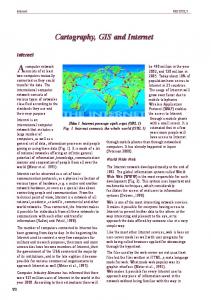
Physics and Technology (Lotov et al, 1991). Now, it is used in computer laboratory work at the Lomonosov Moscow State University and at the Russian University for Friendship of Nations, as well. In addition, the educational environmental computer game LOTOV_LAKE (see Lotov et al, 1992) is based on it. The demo Web resource considered in this paper is based on the same problem, too. A region with a developed agricultural production is considered (Figure 1). The region is placed in a basin of a river which runs through a lake and then into a sea. The lake serves as the municipal water supply. Moreover, the lake is an important ecological and recreational site.
Figure 1. The map of the region
The problem of the further economic development of the region is studied. If the agricultural (here grain-crops) production would increase, it may spoil the environmental situation in the region. This is related to the fact that the application of chemical fertilizers and water for irrigation may increase the grain-crops output substantially, but at the same time may result in negative environmental consequences: • a part of the chemical fertilizers may find its way into the river with the withdrawal of water, • a shortage of water in the lake may occur during the dry season because of the irrigation. Two agricultural zones exist in the region. In the upper zone (higher than the lake), irrigation and fertilizer application may directly result in a drop of the lake level and in the increment of water pollution. Irrigation and fertilizer application in the zone which is lower than the lake also may influence the lake, but indirectly: irrigation and fertilizer application in the lower zone may result in the need for additional water flow from the lake into the river (the release is regulated by the dam) to fulfill the requirements of pollution control at the point A in Figure 1. A finite number of grain-crop production technologies are considered. Intensive technologies are related to high level of water consumption and fertilizer application. Several technologies are related to low water consumption and fertilizers application, but the production is low, too. Technologies which use moderate amounts of water and fertilizers result in a moderate output. Reasonable strategies of agricultural production and of water release through the
122
dam should be developed. Different economic and environmental indicators represent different interests: farmers are mainly interested in grain-crop production while recreational business is mainly interested in the level of the lake, and the inhabitants of the city are mainly interested in the water quality. So, we consider three performance indicators (choice criteria): • agricultural production, • level of the lake, • water pollution in the lake. The mathematical model is described in Appendix 1. The IDM technique is introduced first schematically (Figures 2-4), and only then we provide real decision maps related to the problem (Figures 5-7).
Figure 2. The set (variety) of feasible goals and its efficiency frontier
Figure 3 . The Edgeworth-Pareto Hull
Figure 4. The decision map
First, let us consider the first two criteria only. In Figure 2, possible (feasible) combinations of the production and of the level of the lake may be displayed: the value of production is given on the horizontal axis and the value of the level of the lake is given on the vertical axis. Actua lly, the frontiers of the variety of feasible combinations of two criterion values are depicted. For any combination from the variety, computer can calculate a feasible strategy of regional agricultural production and water release which will result in it. Therefore, the variety of feasible combinations of criterion values 123
displayed in Figure 2 may be denoted as the set (variety) of feasible goals expressed in terms of these criteria. This set is known in the decision theory as the feasible set in criterion space, the FSCS. Since the increase of both criterion values is preferable, the efficiency (nondominated) frontier of the FSCS is of interest. It is given in Figure 2 by the curve AB (the "north-eastern" frontier in this case). By this, the efficient tradeoff between criteria is displayed as well. For example, the efficiency frontier in Figure 2 shows how the level of the lake may be transformed into production, if the efficient subset of strategies is used. It is said that the efficiency frontie r provides the efficient tradeoff between two criteria. For this reason, this frontier may be helpful during decision making and negotiations. The idea to display the efficient tradeoff among two criteria was introduced by Gass and Saaty (1955). Display of efficient frontier is a main part of so called in multiple criteria decision methods (see Cohon 1978). In the case of three, four and greater number of criteria, the efficient tradeoff between criteria can not be displayed so easily. To do it, the Interactive Decision Maps technique was developed. To introduce the concept of the IDM, let us return to Figure 2 and modify the picture slightly. In Figure 3, a new set which contains, along with the feasible goals, all dominated (including non-feasible) combinations of criterion values is depicted. The variety of the additional non-feasible points is shaded. In accordance to Stadler (1986), we denote the broadened set as the Edgeworth-Pareto Hull (EPH) of the set of the FSCS. Note that the efficiency frontier (the "north-eastern" frontier in this case) of the broadened set remains the same, but dominated frontiers disappear. It is not important whether the original FSCS or its EPH is depicted if only two criteria are considered, but the EPH is very important in the case of three and more criteria. Let us now consider the water pollution as well. In this case, one may obtain several EPH for two criteria related to different restrictions imposed on the value of the third criterion (pollution is restricted by several numbers). Then, several two-criterion EPH may be superimposed. They are given in Figure 4 where the maximal EPH corresponds to the EPH in Figure 3 for which no restrictions on the pollution have been imposed. Note that the efficiency frontiers in Figure 4 do not intersect. For this reason, different efficiency frontiers may be loosely placed in the same picture without interfering each other. Collection of the efficiency frontiers comprises a decision map. Decision maps technique is the multiple criteria decision aid technique developed for the case of three choice criteria (see, for example, Haimes et al. 1990, p.71) where several cross-sections of the efficiency frontier of the feasible set in criterion space are superimposed. The Interactive Decision Maps (IDM) technique applies the concept of a modified decision map: efficiency frontiers of two criteria related to several restrictions imposed on the value of the third criterion are depicted. Changing one efficiency frontier for another, one can see how the restriction on the third criterion influences the efficient tradeoffs between two first. A modified decision map thus helps to understand the efficient tradeoffs between all three criteria. Though modified decision maps used in the IDM technique are very close to usual decision maps, they have several advantages. The most important of them is related to the method how modified decision maps are computed. We do not construct various EPH for two criteria. Instead, the EPH for the entire list of criteria under consideration is constructed in advance. Two-dimensional slices of the EPH are then computed and
124
superimposed. The efficiency frontiers of them provide modified decision maps. Since the EPH is constructed in ad vance, various modified decision maps may be depicted on request very fast. The discussion of other differences between decision maps of two kinds are beyond the scope of this paper. For the remainder of the paper, references to decision maps will imply the modified version without additional indication. Since the decision maps differ from usual geographical maps, the common features of them and distinction between them need special discussion. First about the their similarities. Since the efficiency frontiers of decision maps do not intersect (though they may coincide sometimes), they look like the height contours of a usual topographical map. Indeed, a value of the third criterion related to an efficiency frontier of a decision map plays the role of a height related to a contour of a topographical map. This why one can apply his/her knowledge of topographical maps in the case of decision maps. Say, one can see the variety of the combinations of the first and second criteria which are feasible for a given restriction imposed on the value of the third criterion (like ). Moreover, one can easily understand which values of the third criterion are feasible for a given combination of the first and of the second criteria (like ). If efficiency frontiers of a decision map are close, this could mean (like in a topographical map) that there is a steep at this point, i.e. a miserable move of the efficiency frontier results in the substantial change of the value of the third criterion. This information about the efficient tradeoff between three criteria is very important: it means that one has to pay with a substantial change of the third criterion value for a miserable improvement of the values of the first two criteria. Now let us consider distinctions between decision maps and geographical maps. A decision map displays the criterion (outcomes) space: the outcomes of all possible decisions are displayed in one picture, if the number of criteria is three. By contrast, a geographical map usually displays one spatial decision selected somehow in advance in a usual (geographical) space. For this reason, myriad of geographical maps are needed to depict myriad of feasible decisions. A decision map displays all of them at once, but in an aggregated form of feasible outcomes. To select one decision, user has to click on a preferable combination of criterion values in a decision map. Then the efficient decision is computed, and only then it may be displayed in a geographical map. If one would click on the geographical map, additional features of the displayed decision usually are provided (examples are given in the next sections). Distinctions between geographical maps and decision maps constitute a ba sis of their joint application in GIS -based analysis of spatial decision problems. To illustrate distinctions between geographical maps and decision maps, let us consider geographical maps and decision maps used in the educational environmental computer game LOTOV_LAKE (Lotov et al, 1992). They are related to the regional problem introduced above. Usual geographical map of the region is given in Figure 1. Decision maps related to the case of three criteria listed above are given by computer screens provided in the game. Copies of the screens are given in Figures 5-7.
125
Figure 5. One of the decision maps for the regional problem: production versus drop of the lake
Figure 6. Pollution versus production
Figure 7. Pollution versus drop of the lake
In Figure 5, the values of production (measured in thousand tons) are given on the horizontal axis. On the vertical axis, the values of the drop of the level of the lake (measured in feet) are given. Differently colored two-dimensional slices of the EPH for several restrictions on pollution (measured in milligrams of pollutant per liter) are superimposed. Since it is reasonable to decrease the value of the drop, the "south-eastern" frontiers of slices are efficient. They constitute the decision map. The restrictions on pollution are specified in the color scale placed under the decision map. To the left of the decision map, the control panel and the box with criterion values are given. The criterion values in the box are related to the cross given on the dec ision map. The cross displays the current goal which can be moved along the current efficiency frontier or brought to another efficiency frontier. The color of the current efficient frontier is announced above the map and marked out in the color scale under the decision map. Any efficiency frontier in Figure 5 displays the efficient tradeoff between two criterion values. Also, it defines the limits of what can be achieved: it is impossible to increase the values of agricultural production and decrease the drop of the lake beyond the efficiency frontier. The smallest slice is related to minimal, i.e. zeros pollution. Its efficiency frontier shows how the level of the lake may be exchanged for the production while keeping a zero level of pollution. For small values of production (about 24 thousand tons), the maximal level of the lake (drop is zero) is feasible. Then, with the increment of the production, the efficient drop of the level starts to increase more and more abruptly. The maximal (for zero pollution) production value (a little bit less, than 70 thousand tons) is related to the maximal drop of the lake. Note that to achieve the
126
maximal production, it is necessary to exchange a substantial drop of the level for a small increment of production. Other efficiency frontiers have the same shape. Note that as allowable level of pollution increases, the possible production level increases as well. The outer frontier is related to the situation when restrictions on the pollution permit maximum efficient concentration. Note that if the drop of the level of the lake is relatively small, the efficiency frontiers are close they coincide practically. This means that a substantial decrement of pollution does not result in serious economic disadvantages for these levels of the lake. Two different decision maps are given in Figures 6 and 7. Pollution versus production and pollution versus drop of the lake are given in Figures 6 and 7, respectively. Suppose that a preferable feasible goal, i.e. a point on an efficiency frontier, has been identified by user. Then, the related decision is computed and displayed in the geographical map. In Figure 8 the geographical map of the region augmented with information about the computed decision and its outcomes is provided. The distributions of the areas of two agricultural zones among technologies are shown by two circular diagrams (relation between color and the number of technology is given in color scale). A column diagram placed near the dam shows the water release through the dam. Other column diagrams and several inscriptions inform about outcomes of the decision (grain crop production, level drop and pollution) as well as about other values of minor importance. The inscriptions in the right lower corner are related to the educational nature of the software: they provide comments to the decision and its score. In general, score is between zero and ten. One can see, that the score of the decision displayed in Figure 8, is not too high. Though it is efficient (since the goal chosen by user is efficient in any case), authors of the game consider it to be not sufficiently good.
Figure 8
Figure 9
In Figure 9, another decision is given. Though agricultural production is less than in Figure 8, pollution and drop of the level of the lake are quite small. For this reason, the decision is evaluated by authors to be excellent (score equals to ten). Surely, score is not given in real- life problems, and so user is solely responsible for identifying reasonable goals. The educational environmental computer game LOTOV_LAKE (for DOS) is available at http://www.ccas.ru/mmes/mmeda/soft/. The sample study area shows that we had to use two different displays of the GIS to inform about two decisions of the game. In contrast, all efficient decisions are displayed in aggregated form by one of decision maps given in Figures 5-7. Any of them would be sufficient for it. The IDM
127
technique has been used here to provide arbitrary arrangement of criteria in decision maps. Moreover, one could change the number of tradeoff curves and zoom a map (an example of zooming is given in the next section). The role of the IDM technique is much more important in the case of four, five and more criteria. In the latter case, a decision map related to restrictions imposed on the values of the fourth, fifth and other criteria ma y be displayed immediately after the request. Moreover, in the case of four criteria, one may display several decision maps (for several variants of restrictions) in a row. For any decision map in the row, the restrictions imposed on the fourth criterion can be chosen automatically or by user. Any criterion may be chosen as the fourth one, and the restrictions may be changed easily. In the case of five criteria, a matrix of decision maps may be displayed. Let us consider an example. In addition to above three criteria of the regional development problem, we consider agricultural production in the upper zone measured in thousand tons and pollution concentration in the river near the mouth measured in milligrams of pollutant per liter ("sea pollution"). In Figure 10, a matrix of decision maps for this problem is displayed. It consists of decision maps, any of which, like decision map in Figure 5, displays efficient tradeoffs between the first three criteria. Color scale which is now common for all decis ion maps is given under the matrix. Any decision map is related to certain restrictions imposed on the value of agricultural production in the upper zone () and on the value of sea pollution (). The restrictions on agricultural production in the upper zone and on sea pollution are given near columns and rows of the matrix. A restriction on agricultural production in the upper region which is given above a column is the same for the decision maps in this column. A restriction on sea pollution which is given to the right side of a row, is the same for the decision maps in this row. Note that the influence of the restriction on agricultural production in the upper zone is much higher than of the restriction on sea pollution. Nevertheless, the influence of sea pollution is visible as well: maximal production values can not be achieved if sea pollution is less than 10 mg/l.
Figure 10. Decision map matrix
128
In Figure 10, there are 7x9 decision maps in the matrix. The maximal number of rows and columns in a matrix of decision maps depends on display quality only. Let us stress once again that a matrix of decision maps can be displayed very fast: an updated matrix is displayed in a few seconds after a collection of values of the fourth and the fifth criteria has been set or changed. Moreover, one can easily change the list of three criteria for which efficient tradeoffs are displayed in decision maps. This can be done by simple operations. The updated matrix will be displayed in a few seconds, too. Another approach in the case of four, five or more criteria is animation of decision maps. Animation of a single decision map is based on a monotone increment (or decrement) of, say, the fourth criterion. Moreover, animation of a row or of an entire matrix is possible, too. In these cases, the value of the fifth (sixth, seventh) criterion may be changed step by step. All these approaches are related to the fact that the EPH has been constructed in advance. Unfortunately, animation of decision maps can not be illustrated in the paper. We can propose to download the demonstration version of the software Visual Market/2 from our Web pages (http://www.ccas.ru/mmes/mmeda/soft/) and to try to use animation of decision maps. This software is based on the same visualization technique, but applies another goal method the Reasonable Goals Method considered in section 3. 3. Feasible Goals Method and its real-life application The goal method is a well known approach to decision making with multiple criteria. In the goal procedures, the user identifies a goal, and then a decision is computed. As a rule, the variety of feasible goals is not displayed in the framework of the goal procedures (see, for example, Charnes and Cooper 1961, Steuer 1986, etc.). These results in a sophisticated question: What decision should be provided if the goal identified by user is not feasible? To solve this problem, a feasible criteria combination of criterion values closest to the identified goal is usually computed. A related decision is computed, too. If the closest feasible combination is distant from the identified goal, user may be disappointed with the result. Moreover, the feasible combination of criterion values closest to the identified goal (and the related decision) may depend more upon what is understood under the distance than on the goal, and so the computed decisio n will disregard the preferences of user. As it was shown above, we display of the variety of all feasible goals to avoid this problem. Due to this, the above problem vanishes. The set of feasible goals is displayed in the form of the FSCS or its EPH introduced in the previous section. Only then an opportunity to identify a preferable goal is provided; the related decision is computed and displayed in GIS. The method based on this idea was introduced in 70s (Lotov 1973 ) and is now denoted as the Feasible Goals Method. Till the end of 80s, it was used without IDM technique which did not exist that time. Instead of it, collections of decision maps and other pictures containing efficient tradeoffs between two criteria were prepared in advance (see Lotov 1984). Now the IDM technique is used to inform user on the variety of feasible goals. It helps to identify a feasible goal as well: a preferable feasible goal may be identified by a mouse click on an appropriate decision map. The main steps of the IDM/FGM technique for spatial problems are (see Scheme 1): 1. construction the EPH;
129
2. interactive display of decision maps; 3. identification of a preferable feasible goal; 4. computation of an efficient decision which should lead to the chosen goal and its display in GIS.
Scheme 1. The scheme of the IDM/FGM. Computer processing is denoted by C and decision maker by DM.
The FGM technique has been used for screening possible decis ions in several problems, including: • development of the national social-economic goals and strategies of long-time economic growth in the USSR (Lotov 1984); • development of the strategies of economic reform in Russia (Kamenev and Kondratiev 1992); • development of the international strategies of the atmosphere pollution abatement (Bushenkov et al. 1994a); • development of the response strategies to the global climate change (Lotov 1994); • development of the strategies of water quality improvement ( Lotov et al. 1997a). These and other applications of the FGM technique are collected in the book ( Lotov et al. 1997b). Three latter problems were related to development of spatial strategies, and so GIS were used for the display of them. The last problem provides an example of a real- life application of the FGM/IDM technique jointly with GIS: a computer-based system for supporting the water quality planning in river basins was developed on request of the Russian State Institute for Water Management Projects (now private Institute for Water Information Research and Planning, Inc.) and used in this Institute for several years. The detailed description of the system was published in ( Lotov et al. 1997a). Here, we describe it in short. In this problem, the recommendations must be made regarding to the wastewater treatment in the industries and the municipalities in a river basin. To obtain a moderate investment, environmental engineers need to prove to the stakeholders (federal, regional and municipal aut horities as well as owners and management of industrial enterprises) that the investment will result in a substantial improvement of the environment. Earlier, environmental engineers have applied optimization procedures to obtain plans related to the minimal cost that met medical and ecological requirements. Calculation of the optimal plan was fulfilled on the basis of a mathematical model of pollution transport and wastewater treatment. Often it was impossible to find a feasible plan which met the requirements, and so environmental engineers had to change these requirements somehow. Moreover, in the cases when plans have been found, they were of too expensive to be fulfilled during 80s and certainly they have nothing to do with the real
130
life now. Therefore, environmental engineers had to the optimal plans by the deleting of several investment decisions from the plan in accordance to their experience. This has resulted in inefficient strategies which have been sharply criticized. This is why a new decision support technology of water quality planning was requested and elaborated in the form of a computer-based decision and negotiation support system. In this system the measures devoted to the water quality improvement were split into two phases: 1. implementation of a reasonable balance among cost and pollution which is found by screening of myriad of feasible plans; and 2. final resolution of water quality problem. The computer-based support was related to the first phase. Along with the cost criterion, several water quality criteria were incorporated into the analysis. The FGM/IDM technique was used for display of the efficient tradeoff between cost and several pollution criteria. After exploring various decision maps, engineers had to identify several feasible goals and receive related investment strategies. These strategies were displayed in a specially developed GIS. Rivers under consideration were assumed to be split into a finite number of reaches separated by monitoring stations. The production enterprises were grouped into industries which included the enterprises with analogous production technology and pollutant output structure. Municipal services were grouped in the same way. Moreover, the production enterprises and municipal services were grouped in accordance to the reach they belong. The problem was reduced to planning of investment for constructing the wastewater treatment facilities. The investment (not given in advance) was allocated among production industries and municipal services in reaches of the river. The integrated mathematical model used in the system consisted of two parts: • a collection of industrial wastewater treatment models; any model related the decrement of pollutants emission to the cost of wastewater treatment in a industry or a service. The models applied the same idea of technological description (Koopmans 1957) which was used in this paper in the regional model. A decision variable described the fraction of wastewater, which should be treated by a certain wastewater treatment technology in a given industry or a service placed in a given reach; • a pollution transport model which provided an opportunity to calculate concentrations of pollutants at monitoring stations for a given discharge. Sinc e more than twenty pollutants were usually considered, environmental engineers used grouping of the pollutants to obtain aggregated environmental criteria. The values of criteria were measured in relative units. The ideal value of an environmental criterio n was one. Four following pollution criteria were considered: • fishing degradation criterion; • toxicological criterion; • sanitarian criterion; and • general pollution criterion. So, five criteria (four pollution criteria plus one cost criterion) were considered in the system. It was desirable to decrease the values of all criteria. To study the efficient tradeoffs among criteria, environmental engineers explored matrices of decision maps. One of the matrices of this kind is given in Figure 11.
131
Figure 11. A matrix of the decision maps. The value of the sanitarian indicator changes from column to column. The value of the toxicological indicator changes from row to row.
This figure is a copy of the display of the system, and so the inscriptions are in Russian. The system was coded in DOS. For this reason the matrix consists of nine decision maps only. Any decision map is related to certain restrictions imposed on general pollution (values are given to the left of rows) and on sanitarian criterion (values are given under columns). Any decision map displays superimposed colored slices of the EPH. Values of fishing degradation criterion are given on horizontal axis, and values of toxicological criterion are given on vertical axis. Colors are related to the cost of the plan. The cost is given the scale under the matrix, it is measured in millions of USSR rubles in 1989 (R10 = $1, approximately). Comparing the decision maps for properly chosen restrictions imposed on general pollution and sanitarian criterion, one can understand the influence of these criteria and select a preferable decision map. By this the values of row and column criteria are fixed. Then, a preferable goal may be identified on the decision map and the related strategy computed. Let us consider an example. Though the river is quite polluted, the value of sanitarian criterion is sufficiently good in all columns. For this reason, the left column may be chose n. The matrix shows that a reasonable value of general pollution criterion may be achieved only if sufficiently large cost (green color) is applied. Let us choose the decision map in the upper row given in Figure 12.
Figure 12. A decision map for water quality planning
Figure 13. A zoomed part of the decision map
132
As one can see, the influence of additional cost on the efficient frontier of fishing degradation criterion and toxicological criterion is displayed without necessary details in this figure. Since the IDM technique provides an opportunity to zoom a part of a decision map, it is possible to explore this influence in details. In Figure 13, a zoomed part of the decision map is given. It is clear that the additional cost (yellow and brown colors) may be used for decrement of the fishing degradation criterion, but the toxicolo gical criterion can not be improved substantially. It is clear that the marginal efficiency of investment falls (just compare decrement of fishing degradation due to change from green to yellow and from brown to red which are related to the same additional cost). The goal indicated by the arrow in Figure 13 was chosen by environmental engineers. A related investment strategy was computed and displayed in a specialized self- made GIS. Examples of the GIS display are given in Figures 14 and 15. Environmental outcomes of the strategy are displayed in Figure 14. On the geographical map of the basin (this is the Klyazma river basin which is to the north-east from Moscow), the monitoring stations were given by small squares placed along the river and its inlets. To receive information about a particular monitoring station, one had to zoom the related square. The square related to the monitoring station number 2 was maximally zoomed in Figure 14. It contains column diagram representing the concentrations of particular pollutants. The relation between color and the name of the pollutant is provided in the left corner. Concentrations are given in relative values: the recommended maximum concentration equals to one. The horizontal red line crossing the column diagram displays the recommended maximum concentration. The arrow points out one of the pollutants which has a high concentration. Detailed information on this pollutant is given in the box placed in the upper right corner: the name of pollutant (suspended staff in this case), its concentration in milligrams per liter, its concentration in relative units and the recommended maximum concentration. Zooming of squares related to the monitoring stations were provided by a mouse click. So, mouse clicks had different outcomes in the case of the geographical map as compared to a decision map.
Figure 14. Environmental outcomes of the investment strategy
133
Figure 15. The investment allocation.
The investment allocation is given in the geographical map displayed in Figure 15. The information display has the same feature: one has first to zoom one of the squares. Here monitoring station number 2 is considered once again. This time the investment structure in the reach placed up to the monitoring station is given in the square. The total investment value is displayed above the column. The relation between colors and the names of the industries are given in the left corner. Here, the maximal investment volume in the reach is given by dark green color. It is pointed out by the arrow. The name of the industry (here the municipal water discharge) and the volume of investment are given in the box in the upper right corner. Let us now consider the computer-based system for supporting the water quality planning as a whole. The system consisted of five main subsystems: 1. Data preparation subsystem; 2. Subsystem for constructing the EPH; 3. Subsystem for exploration of the EPH and identification of feasible goals; 4. Subsystem for investment strategies computing; 5. Subsystem for strategies display (GIS). Here we have considered the third and the fifth subsystems which illustrate the idea of the paper. Data preparation subsystem is pretty standard. The mathematical basis for the second and the fourth subsystems is outlined in short in Appendix 2. Environmental engineers used to construct several reasonable variants of the plan which they provided to the stakeholders, i.e. federal, regional and local authorities as well as the owners and management of industrial enterprises. By this they hoped to improve the stakeholders' understanding of the situation. Actually, environmental engineers played a role of experts who screened the variety of feasible investment strategies and identified several of them. Application of the FGM/IDM technique helped them to screen the strategies on the basis of the information on potentialities of choice and on efficient tradeoffs. GIS helped to display the selected plans and their outcomes in a simple form. By this, these techniques helped environmental engineers to defend the proposed plans of environmental investment.
134
4. Reasonable Goals Method and its applications If the EPH of the feasible goals set is convex, decision maps are simple and may be understood quite easily. In the opposite case, assessment of the efficient tradeoffs is not so simple. To avoid this complication, the Reasonable Goals Method may be used instead of the FGM. In the RGM, the convex hull of the EPH (the Convex Edgeworth-Pareto Hull, the CEPH) is constructed and displayed by the IDM technique. User has to explore decision maps which look like the decision maps for convex problems. A goal is identified in the same way as in the FGM. The main problem is related to the fact that, in contrast to the IDM/FGM technique, the goal in the IDM/RGM technique may be not feasible. Although, the goal belongs to the convex hull of the feasible goals set, and therefore its points are linear combinations of feasible goals, the goal itself is not necessarily feasible. Let us consider an example of two criteria (cost and benefit) and a finite number of variants (this is the simplest exa mple of the non-convex problem). In this case, the feasible goals set is given by a finite number of points in criterion space (Figure 16). The CEPH is shaded in Figure 16. User is provided with the CEPH, but not with the variant points. User may identify a most appropriate goal in the shaded space, but the identified goal only occasionally may be feasible when it coincides with one of the points. It is interesting to note that the efficient frontier of the CEPH coincides with the well-known cost-benefit curve. Cost-benefit analysis is often not sufficient for decision support, especially in public problems (see Dorfman 1996). Indeed, it is unable to consider several benefits (say, separate benefits of different population groups) and several costs. In addition, uncertainties or inaccuracies of estimates can not be incorporated directly into the cost-benefit analysis. So, multiple criteria development of the cost-benefit analysis is needed. This was done in the IDM/RGM technique.
Figure 16. The CEPH for two criteria and a finite number of variants.
The idea to support the identification of a reasonable goal was applied to finite choice problems by Lotfi et al. (1992). They help to identify the goal close to the efficient variants in attribute space, by displaying those variants which are not worse than aspiration levels identified by user (additional statistical information is provided to user as well). In contrast, we use decision maps for supporting the identification of a reasonable goal. Actually, the CEPH is treated as the variety of reasonable goals. User is informed about it and its efficiency frontiers with a help of the IDM technique. User has to express his /her preferences by identification of a reasonable goal. The information is used for selecting a small number of variants which are in line with the identified goal.
135
The scheme of the IDM/RGM technique is given in Scheme 2. Note that, in contrast to the FGM, several variants are selected (instead of one decision in the convex case).
Scheme 2. The IDM/RGM technique. Computer processing is denoted by C and decision maker by DM.
Selecting of several variants from the initial set on the basis of the reasonable goal is based on the following idea. The identified goal is considered to be a combination of aspiration levels. This means that we suppose that the user would prefer to achieve the identified levels of criterion values rather than to receive a criterion value which is better than the identified level. In the case of a finite number of feasible decisions, two options may occur: 1. there exist variants which are not worse than aspiration levels identified by user; and 2. such variants do not exist. In the first case, we loosely select those variants and display them to user. If such variants do not exist, we use the following idea: a modified point is related to any original feasible point. The meaning of aspiration level is used for constructing the modified points: if the original criterion value in a point is better than the aspiration level, the aspiration value is used instead of the original value. The n, usual Pareto domination is applied to modified points: non-dominated points are selected among them. Finally, the original feasible points which gave rise to selected modified points are displayed to user. Figure 17 provides an illustration for the case of two criteria which are subject of maximization.
Figure 17. Binary relation used in the RGM technique.
The original feasible points are given by black circles, and the reasonable goal is denoted by a star. For any original point, a modified (white) circle is constructed (say, point 1' for point 1, etc.). The criterion value of a modified point equals to the minimal of two values: the criterion value of the original point and the aspiration level. If criterion values for an original point are less than the aspiration levels (like point 3), the modified point coincides with the original one. Pareto domination is applied to the modified points. Point 2' dominates (is better, than) point 1', and point 4' dominates point 5'. So, three nondominated modified points are left: 2', 3, and 4'. For this reason, points 2, 3 and 4
136
correspond to the choice of the reasonable goal given by the star. They are displayed to user. The case of finite number of feasible decisions is very important since it is related to visual exploration of various databases and selection of a small number of preferable items stored in them. Let us consider an usual relational database. Items (say, decision variants like location of business in a region) are given by rows (tuples) of the database. The items are described by their attributes given in columns (fields) of the database. Several numerical (cardinal) attributes may be chosen by user to be the selection criteria. The FSCS is given by variety of points in criterion space which correspond to the rows of the database. The CEPH may be approximated and displayed by means of the IDM technique. Then the RGM may be applied for the selection of variants from the database. Let us consider an example. In this example, the IDM/RGM technique is used as decision support tool in GIS which helps to select a small number of variants. The problem of selecting a location for rural health practice is considered. Earlier a spatial decision support system which should help health practitioners to make decision was developed (see Jankowski and Ewart 1996). This system was based on the multiple criteria methods traditionally proposed for decision support. Data representing healthcare, social, economic, and environmental information were aggregated by 47 Primary Care Service Area (PCSA) encompassing the entire state of Idaho. The attribute database describing the PCSA provided information for evaluation criteria. Professional criteria included the need in physicians denoted by DOCS, population in the year 1990 (POP90), percent receiving Medicare and Medicaid (MEDICARE), fertility rate (FERTILITY), whether loan repayment program is approved in the area (LOAN_REPA), how much time a physician has to spend a week on call (ON_CALL), etc. Personal criteria include percent of unemployed (UNEMPLOYED), percent below poverty level (POVERTY), percent with college degree (POP_DEGREE), etc. The IDM/RGM technique was adapted to the problem. To illustrate joint application of the IDM/RGM technique and GIS, we outline this study in short (it will be described in details elsewhere). In Figure 18, the initial display is provided. A part of the PCSA database is given.
137
Figure 18. A part of the PCSA database
Any possible PCSA is described by a number of attributes (only a part of them is displayed). Along with Jankowski and Ewart (1996), these data were included in an ArcView (TM) project view file and represented in a map of Idaho. The PCSA locations are given by green points on the map. By a mouse click, one can get information on a certain PCSA. Figure 18 displays such information for Twin Falls, Idaho. To illustrate the application the IDM/RGM technique, we use five attributes for the selection criteria: • need in physicians (DOCS) to be maximized; • population in the year 1990 (POP90) to be maximized; • a time a physicia n has to spend a week on call (ON_CALL) to be minimized; • fertility rate (FERTILITY) to be maximized; • percent below poverty level (POVERTY) to be minimized. Matrix of decision maps for the problem of selecting a location for rural health practice is give n in Figure 19.
138
Figure 19. Matrix of decision maps for the problem of selecting a location for rural health practice
Any decision map displays the efficient tradeoff between DOCS, POP90, and ON_CALL. Values of the first two criteria are given on axes, and values of ON_CALL are given by different shadings. Relation among shading and the value of ON_CALL are provided in the scale to the right of the matrix. Any column of the matrix is related to a certain restriction imposed on FERTILITY (), and any row is related to a certain restriction imposed on POVERTY (). Due to this, one can understand how the restrictions imposed on fertility rate and percent below poverty level influence the feasible values of DOCS, POP90 and ON_CALL. Moreover, influence of the restrictions on efficient tradeoff between these criteria is clear as well. Note once again that the restrictions may be changed easily to make the matrix more informative. In the decision maps for which fertility rate is not less than 60 and percent below poverty level is not greater, than 20, a reasonable goal was identified (DOCS = -11.58, POP90 = 111,755, ON_CALL = 1). It means that a person who identified it, was not afraid of a high competition, prefered to live in a populated place, but did not like to spend too much time on call. After the goal has been set, the related PCSA were computed immediately. They are provided in Figure 20. First of all, variants which are not worse than the identified goal, do not exist for this goal. For this reason, Pareto domination of modified points was used. It resulted in four PCSA: St.Maries, Weiser, Nampa and Boise. One can see that Nampa is the only PCSA which is close to the identified goal (by the way, the need in physicians is much better that it was required). Since the software does not know the preference tradeoff of user, it displays three different PCSA whic h are in line with the identified goal and may happen to be better than Nampa. Note that in Nampa one has to spend 1.29 hours on call instead of one hour in the identified goal. In St.Maries one has to spend on call only 0.92 hours a week. Perhaps, user wo uld agree to sacrifice the population level for this advantage? In any case, this option is provided. Weiser was selected since it is a little bit larger than St.Maries. Finally, Boise, the capital of Idaho, was chosen since Nampa does not satisfy the population requirement precisely. Perhaps this is important for user? In any case, user
139
has to choose from the given list of PCSA by himself. It is important that all other PCSA are not in line with the identified goal, and so they were not selected and displa yed.
Figure 20. The PCSA related to the identified goal
To help user to choose from the given list of PCSA, the map of GIS is provided. In the map the selected PCSA (given in green) and the PCSA which were not selected (given in red) are discerned. One can click on a selected (green) PCSA, and the data about it will be displayed like in Figure 18. In principle, any additional information about the PCSA, including photos, films, etc., may be provided along with other multimedia tools. Application of the IDM/RGM technique for screening of varieties of variants given by their attributes in various databases is only one possible application of it. Another example is provided by exploration of finite decision problems described by non-linear mathematical models. In this case, the attribute values are not given in advance, and so they should be computed by a mathematical model. Actually, preprocessing consisting in the computing of attribute values for all decision variants is needed. The idea of the IDM/RGM technique in the case of a finite number of variants was introduced in (Bushenkov et al 1994b, Gusev and Lotov 1994). In the above problem, database contained less than 50 variants. In different studies, the IDM/RGM technique proved to be effective for up to several thousands of decision variants. Normally, the number of selected elements is rather small and may be about twenty for several thousand of variants evaluated by, say, five criteria. Everything depends upon the geometry of point set. If the number of items is about several millions, the CEPH can be constructed as well, and so IDM/RGM technique may be applied, too. Problems of extracting useful information from large databases are the subject of a new field of computer science data mining (see Fayyad et al. 1996). This example shows that the IDM technique may be used in this field, too. In the case of a non-linear mathematical model describing decision problems with infinite number of decision variants, methods for stochastic approximation of the FSCS
140
may be used (Kamenev and Kondratiev 1992, Bushenkov et al 1995 ): the set of feasible decisions is approximated by a large finite number of variants. Then the criterion values for these variants are computed. In this case, the CEPH for the original model is stochastically approximated by the CEPH for a finite system of points in criterion space. After that, the above screening of the variety of decision variants given by the criterion values can be applied. 5. IDM technique in INTERNET resources for developing independent solutions of public problems The IDM/FGM and IDM/RGM techniques may be implemented in computer networks. Due to this, new opportunities which have not been feasible earlier may be provided for users of computer networks. In this section, we consider one of them related to the open computer network Internet: Internet -based support for development of independent solutions of important public problems. The Internet provides new enormous opportunities for millions of people to exercise the (see Williams and Pavlik, 1994), i.e. to receive information directly from the sources, independently from mass media which inevitably have to screen it (i.e., to distort it). For example, a special Internet server containing full objective information about a particular important public problem may be established. But, if somebody would like to apply the to the information on possible solutions of the above problem, he/she will find that the free access to the original information alone is not sufficient it doesn't answer the question. Special methods for providing objective information on possible decisions should be supplemented. Since these methods are supposed to be used by ordinary people, they should be simple and implementable in the wide-spread Internet tools. The IDM/FGM and IDM/RGM techniques satisfy these requirements. Let us co nsider the example Internet resource provided now on the Web pages of the Department of Mathematical Methods for Economic Decision Analysis at the Computing Center of Russian Academy of Sciences (http://www.ccas.ru/mmes/mmeda/resource/). The code has been developed on the basis of the Common Gateway Interface scripts (CGI-scripts). The CGI-scripts provide a tool for generating Web-pages, possibly using user-supplied information (see WWW Consortium). Web search systems (like AltaVista, Lycos, WebCrawler) are examples of systems based on the CGI-scripts. It is important that a CGI-script is stored on a server and is never downloaded to the user's computer. Due to this feature: 1. user can work in any OS (Windows, Macintosh, UNIX, etc.); 2. information is stored and updated by the authors; 3. no time is wasted on downloading the software since the user interface is provided by a Web-browser and the INTERNET interface by the Web-server. Therefore, all advantages of the client-server scheme are utilized here. A CGI-script can be written in any programming language. It gets the information in the text form from the standard input and environment variables and yields information to the standard output. To apply an interactive CGI-script, a so-called form is organized in a Web-page by the means of HTML. A form is a set of control elements which are related to a CGI-script processing the user input. A form looks and behaves like a Windows dialog box, but it doesn't appear in a separate window: instead, it is embedded into a WWW-page. Pushing
141
a button in a form causes a jump to a page generated by the CGI-script according to the user input. The interactive CGI-scripts may be used for implementing the IDM/FGM and the IDM/RGM techniques jointly with geographical maps of a GIS. In the case of the IDM/FGM and the IDM/RGM techniques, user-supplied information is the control of the IDM and the position of the identified goal. The example Internet resource is actually a CGI-script coded in C programming language in UNIX environment. Since the user interface is limited in the CGI-scripts by push buttons, radio buttons, check boxes, text input fields and points clicking on pictures, we had to limit ourselves with these tools. For this reason, the scroll-bars which are applied in the IDM software (in WINDOWS environment) very intensively have not been used. These are disadvantages of the application of the CGI-scripts. For this reason, now we are planning to apply new tools which will provide an opportunity to use the IDM technique in full scale. The simplest way to demonstrate the opportunities of the new kind of Internet resources is based on display of several prepared decision maps for three criteria (without animation). We have done it for the example problem considered in section 1. The relations between the agricultural production, the level of the lake, and the water pollution are displayed by several decision maps. By this, the user is informed about potentialities of choice for these criteria. Then, user can choose an appropriate decision map and identify a preferable feasible goal point by a mouse click on it. The Web-server computes then the related decision and displays it to user using a GIS. The user needs only Internet access and the Web-browser. No additiona l software is required. Note that this is an example of the Internet resource. Application of resources of this kind will exercise the right to know the information on possible solutions of public problems, say, strategies for regulating of a natio nal economy or strategies for solution of local, regional, national, or global environmental problems. Ordinary people will receive opportunities to develop independent decisions. This may help ordinary people to understand decision making problems faced by local or other authorities. From another point of view, this may induce people to try to control decision processes actively. In turn, this may contribute to the progress of civic society. The resources described above can be used for education as well. Students will use Internet to assess real- life public problems by developing their own solutions. Moreover, resources of this kind may be considered a prototype of new active tools which may be a part of electronic mass media of the future informa tion society. 6. Conclusions The above Internet resource for independent decision making is one example how the IDM technique can be applied on the Internet. Different applications are possible, too. In particular; the IDM technique can be used in Internet-based negotiations. The idea applies the concept of Principled Negotiations (PN) outlined in Introduction. We consider the case when the search for a coordinated decision may be based on the exploration of a mathematical model or a database of possible alternative solutions of the problem. Surely, in this case the model or database should reflect a shared vision of the situation (see Loucks et al. 1996 ), and interests of negotiators should be related to performance criteria described in the model or attributes given in the database. The study of a decision problem described by a shared model or database, differs from the study of, say, purely
142
political topics: in our case, a decision providing a balance of interests may be found by screening the variety of feasible decision variants. For this reason, the PN concept can be implemented in this case on the basis of the IDM technique. Here we exemplify this idea by a particular, but very important topic: negotiations on Locally Undesirable Land Use (LULU). Actually, every proposed land use is potentially a LULU (Couclelis and Monmonier 1995) and may result in Not In My Backyard (NIMBY) syndrome. Beardsley (1992) identifies NIMBY to be a prime reason for the recent drastic increases in waste disposal costs. Therefore, new computer tools which can help to resolve the sophisticated public problems of this kind seem to be extremely important. Since land use is a natural spatial problem, various GIS may play an important role in this field (see, for example, Shiffer 1992, Couclelis and Monmonier 1995, Jankowski et al. 1997). Usually the GIS-based negotiation support tools are used for supporting the position-oriented negotiations. This is related to the nature of GIS which provide fantastic opportunities to display particular proposals of negotiators, but they can not be used directly in PN for the search among all possible decision variants. Combination of GIS with the IDM technique may help to use GIS in PN. This is especially important, since PN seems to be the tool which may solve the LULU problems. Indeed, PN may be used for the search of solutions providing efficient combinations of unanimous public interests. In this case, PN will take into account recognized public interests, but will refuse to consider private interests related to private backyards. So, PN will be fair, and due, to the application of the IDM technique, they can be arranged in a transparent form. Since the main issues related to the LULU problems are fairness and efficiency of the decision (Susskind and Cruikshank 1987), PN may be helpful in this case. The Internet provides additional opportunities for dealing with the LULU problems: people can explore them at home and at the most appropriate moment. It is clear that this may help to involve people into the problem resolution. Therefore, implementation of PN in INTERNET may provide a new efficient tool for solving the LULU problems. An Internet-based negotiation procedure applying the idea of PN and the IDM technique may consist of following steps. 1. Public interests which will be recognized in the process of decision making are formulated. The list of recognized interests should be shared by local citizens. Specification of recognized interests makes it possible to use the PN. 2. A possibly large list of variants of land use is developed. This job is supposed to be done by objective experts who have no vested interest in the particular problem. Local citizens can check the list of variants and add their own variants. 3. A model describing the consequences of decision variants in terms of recognized public interests is developed (or objective experts who are able to evaluate the decision variants are found). Consequences of all decision variants from the list are evaluated. So, the database of possible outcomes is constructed. This job is supposed to be done by experts as well. The local citizens should have the right to discuss the model and the results. 4. A Web resource devoted to the problem is established. The resource should help to explore the outcomes of the variety of decision variants by the IDM/RGM technique.
143
5. Citizens explore the outcomes of the variety of decision variants displayed in the form of decision maps. To do it, they use usual Web browsers. 6. The initial efficient combination of interests which may reflect the proposal of experts or local authorities is displayed in the form of a point in decision maps. 7. Collaborative decision making consists of steps related to discussion of proposals to move the point (i.e., the current combination of interests) along the efficient frontiers of decision maps. The proposals are developed by particular citizens and announced via Internet. The proposals are approved or rejected by asynchronous voting which may take several days. The winning movement is fulfilled and then new movement proposals are collected. After some time, a current combination of interests becomes final. 8. Several decision variants which are in line with the final combination of interests are constructed and displayed with the help of GIS. Final voting on the selected variants is deciding about the variant which is supposed to be implemented. The above scheme is pretty rough, and it is an proposal for collaboration. It is important to stress that other tools which have been developed in this field earlier, say, Spatial Understanding Support Systems (Couclelis and Monmonier 1995), may be easily combined with the IDM technique. Appendix 1. Mathematical model of the regional problem The production in both agricultural zones is described by a technological model (see Koopmans, 1957) which includes N agricultural production technologies. Let x ij be the area where the i-th technology in the j-th agricultural zone is applied while j = 1 means the upper zone and j = 2 means the lower zone. The areas x ij are non-negative x ij 0 , i=1,2...,N, j=1,2. (1) The areas x ij in a zone are restricted by the total area of the zone bj x ij bj , j=1,2. (2) The outcomes of the application on unit area of the i-th agricultural production technology in the j-th zone is described by the parameters aijk, k=1,2,3,4,5, 1 • aij is the production, • aij2 is the water application during the dry period, 3 • aij is the fertilizers application during the dry period, 4 • aij is the volume of the withdrawal (return) flow, 5 • aij is the amount of fertilizers brought to the river with the return flow. If a distribution of the area among technologies in the j-th zone will be given, it would be possible to calculate the values of performance indicators for the zone zjk = where • • • • •
aijk xij , k=1,2,3,4,5, j=1,2,
(3)
zj1 is the production, zj2 is the water application during the irrigation period, zj3 is the fertilizers application during the irrigation period, zj4 is the volume of the withdrawal (return) flow during the irrigation period, zj5 is the amount of fertilizers brought to the river with the return flow during the irrigation period. 144
It is supposed that water and fertilizers are applied uniformly in time. The water balances are pretty simple. They include changes in water flows and water volumes during the irrigation period. The deficit of the inflow into the lake during the irrigation period equals to z1 2 z14 . The additional water release through the dam during one day denoted by d is supposed to be even during the irrigation period, and so the total additional outflow from the lake during this period equals to d T where T is the length of the dry period in days. For this reason, the level of the lake at the end of the irrigation period Y is calculated as Y = Y0 (z1 2 z14 + d T)/ , (4) where Y0 is the normal level, i.e. the level without irrigation, and is a given parameter. The flow in the mouth of the river near monitoring point A denoted by v Aequals to v A = vA 0+ d (z 2 2 z24 )/T (5) where vA 0 is the normal flow at the point A. The restriction is imposed on the value of the flow v A vA * (6) where the value v A* is given. So, the following restriction is included into the model v A0+ d (z 22 z24 )/T v A * . (7) The increment of pollution concentration in the lake denoted by w L is w L = z15/ (8) where is a given parameter. This means that, computing pollution in the lake, we neglect the cha nge of the volume of the lake in comparison with the normal volume. Along with the restriction on the flow at the point A, the restriction on the pollution concentration at this point is imposed as well w A wA * (9) * where the value wA is given. The pollution flow (per day) in the water at the point A is given by z2 5/T + q A0 (10) 0 where qA is the normal pollution flow. This means that we neglect the influence of fertilizers application in the upper zone on the pollution concentration in the mouth. Then, the pollution concentration at the monitoring point A denoted by wA is computed as w A = (z25 /T + qA0 ) / v A . (11) Taking into account the above expression (7) we receive w A = (z25 / T+ qA0 ) / (v A0+ d (z2 2 z24 ) / T). (12) So, the following restriction is included into the model (z2 5/T + qA0 ) / (v A0 + d (z22 z24 ) / T) w A* , or (13) (z25 /T + qA0 ) wA* (vA0 + d (z22 z24 ) / T). (14) It is important that the restriction (7) is linear, too. So, all expressions of the model (1)(7) are linear. The criterion values are calculated in the following way. The production is a sum of productions in both zones y1 = z11 + z21 . (15) The second criterion is the final level of the lake Y given by (4), and the third one, the additional pollution in the lake, is given by (8). Appendix 2. The IDM technique: mathematical introduction
145
General mathematical formulation of the IDM techniques as follows. Let the decision variable x be an element of decision space W (say, of finite-dimensional linear space Rn ; in this case, decision vectors x are considered). Let the set of feasible decisions X W be give n. Let the criterion vector y be the element of linear finite-dimensional space Rm. It is supposed that the criterion vectors y are related to decisions by a given mapping . (16) Then, the feasible set in criterion space (FSCS) is defined as the variety of criterion vectors which are attainable if feasible decisions are used (17) Let us suppose that user is interested in the increment of the criterion values y. In this case, a criterion point y' dominates a criterion point y , if y ' y and y' y. Then, the nondominated frontier of the FSCS is defined as a variety of non-dominated points of y Y , i.e. such points for which the points dominating them do not exist in Y (the set of dominating points is empty) (18) The Edgeworth-Pareto Hull (EPH) of the FSCS is defined as Y* = Y + (-
)
(19)
where is the non- negative cone of . It is important that the efficiency frontier of the EPH is the same P(Y*) = P(Y), (20) but the dominated frontiers disappear. A two-dimensional slice of the EPH is defined as follows. Let us consider a pair of criteria. Let us denote by u the values of these criteria. Let z* be the fixed values of other criteria. Then, a two-dimensional slice of the set Y* related to z* can be defined as . (21) It is important to note that the slice of the EPH contains such combina tions of the values of the two criteria which are feasible if the values of other criteria aren't worse than z*. The IDM technique is based on approximation of the EPH and on interactive display of decision maps which are collections of frontiers of its two-dimensional slices. Decision maps can be computed and depicted quite fast, if the EPH has been constructed in advance. In the convex case, approximation of the EPH is based on the iterative methods combining the convolution methods due to Fourier (1826) and optimization techniques. The EPH is approximated by the sum of the cone ()and of a polytop approximating the FSCS. The convex hull of the EPH (the CEPH) for a nonlinear system may be constructed on the basis of the same algorithms, if optimization algorithms for the system under cosideration are provided. Short description of the convolution-based algorithms is given in (Lotov, 1996). A more detailed review of mathematical algorithms for constructing the FSCS is given in (Bushenkov et al, 1995). If the IDM/FGM technique is used, the decision maps help to identify a preferable feasible goal. After a non-dominated goal y´ is identified, it is regarded as the
146
(Wierzbicki, 1981), i.e. an efficient decision is obtained by solving the following optimization problem (22) where (23) where
are small positive parameters.
References Beardsley, T. (1991) Waste Not...New Pollution Laws Will be Considered This Spring, Scientific American, 266(4), 143-144. Bushenkov, V.A., Chernykh, O.L., Kamenev, G.K., and Lotov, A.V. (1995) Multidimensional Images Given by Mappings: Construction and Visualization, Pattern Recognition and Image Analysis, 5(1), 35-56. Bushenkov, V., Gusev, D., Kamenev, G., Lotov, A., and Chernykh, O. (1994a) Visualization of Pareto Set in Finite Choice Problem, Reports of Russian Academy of Sciences, 335(5), 567-569 (in Russian). Bushenkov, V., Ereshko, F., Kindler, J., Lotov, A., and de Mare, L. (1982) Application of the GRS Method to Water Resources Problems in Southern Skane, Sweden (Working Paper WP-82-120). Laxenburg, Austria: International Institute for Applied Systems Analysis. Bushenkov, V., Kaitala, V., Lotov, A., and Pohjola, M. (1994b) Decision and Negotiation Support for Transboundary Air Pollution Control between Finland, Russia and Estonia, Finnish Economic Papers, 7(1), 69-80. Camara, A. (ed.). (1995) Proceedings of the 1st Conference on Spatial Multimedia and Virtual Reality. Lisbon, Portugal: New University of Lisbon. Charnes, A., and Cooper, W.W. (1961) Management Models and Industrial Applications of Linear Programming. New York: John Wiley. Cohon, J. (1978) Multio bjective Programming and Planning. New York: Academic Press. Cohon, J.L., and Marks, D.M. (1975) A Review and Evaluation of Multiobjective Programming Techniques, Water Resource Research, 11(2). Couclelis H., and Monmonier M. (1995) Using SUSS to Resolve NIMBY: How Spatial Understanding Support Systems Can Help With the "Not In My Back Yard" Syndrome, Geographical Systems, 2, 83-101. Dorfman, R. (1965) Formal Models in the Design of Water Resource Systems, Water Resources Research, 1(3), 329-336. Dorfman, R. (1996) Why Benefit-cost Analysis is Widely Disregarded and What to do about It, INTERFACES, 26, 1-6. Fayyad, U., Piatetski- Shapiro, G., and Smyth., P. (1996) From Data Mining to Knowledge Discovery: an Overview. In: Advances in Knowledge Discovery and Data Mining, Fayyad et al. (eds.). Cambridge, Massachusets: MIT Press. Fisher, R. and Uri, W. (1983) Getting to YES. New York: Penguin Books. Fourier, J.B. (1826) Solution d'un Question Particuliere du Calcul des Inegalite. Oeuvres II, 317-328.
147
Gass, S., and Saaty, T. (1955) The Computational Algorithm for the Parametric Objective Function, Naval Research Logistics Quarterly, 2, 39. Gusev, D., and Lotov, A. (1994) Methods for Decision Support in Finite Choice Problems. In: Operations Research: Models, Systems, Decisions, edited by Ju.Ivanilov, pp. 15-43. Moscow: Computing Center of RAS, (in Russian). Haimes, Y.V., Tarvainen, K., Shima, T., and Thadathil, J. (1990) Hierarchical Multiobjective Analysis of Large-Scale Systems. New York: Hemisphere Publishing. Jacoby, H.D., and Loucks, D.P. (1972) The Combined Use of Optimization and Simulation Models in River Basin Planning, Water Resources Research, 6(6), December. Jankowski, P., and Ewart, G. (1996) Spatial Decision Support System for Health Practitioners: Selecting a Location for Rural Health Practice, Geographical Systems, 3, 279-299. Jankowski, P., Nyerges, T.L., Smith, A., Moore, T.J., and Horvath, E. (1997) A Spatial Decision Support Tool for Collaborative Decision Making, International Journal on Geographical Information Systems (in print). Kamenev, G., and Kondratiev, D. (1992) A Method for the Analysis of Non-closed Nonlinear Models, Mathematical Modeling, 4(3), 105-118 (in Russian). Koopmans, T. (1957) Three Essays on the State of Economic Science. New York: McGrow Hill. Lotfi, V., Stewart, T.J., and Zionts, S. (1992) An Aspiration Level Interactive Model for Multiple Criteria Decision Making, Computers and Operations Research, 19(7), 671681. Lotov, A.V. (1973) An Approach to Perspective Planning in the Case of Absence of Unique Objective. In Proceedings of Conference on Systems Approach and Perspective Planning (Moscow, May 1972). Moscow: Computing Center of the USSR Academy of Sciences (in Russian). Lotov, A.V. (1984) Introduction into Mathematical Modeling of Economic Systems. Moscow: Nauka (in Russian). Lotov, A.V. (1994) Integrated Assessment of Environmental Problems. Moscow: Computing Center of Russian Academy of Sciences (in Russian). Lotov, A.V. (1996) Comment to the Paper by D.J.White "A Characterization of the Feasible Set of Objective Function Vectors in Linear Multiple Objective Problems", European Journal of Operational Research, 89(1), 215-220. Lotov, A.V. (1997) Computer-based Support for Planning and Negotiations on Environmental Rehabilitation of Water Resource Systems. In: Environmental Rehabilitation of Water Resource Systems, edited by D.P.Loucks, Kluver (in print) Lotov, A.V., Bushenkov, V.A., and Chernov, A.V. (1996) Experimental INTERNET Resource for Development of Independent Strategies, http://www.ccas.ru/mmes/mmeda/resource/ Lotov, A.V., Bushenkov, V.A., and Chernykh, O.L (1992) LOTOV_LAKE. A Scientific Educational Computer Game, http://www.ccas.ru/mmes/mmeda/soft/ Lotov, A.V., Bushenkov, V.A., and Chernykh, O.L. (1997a) Multi-criteria DSS for River Water Quality Planning, Microcomputers in Civil Engineering, 12(1), 57-67.
148
Lotov, A.V., Bushenkov, V.A., Chernykh, O.L., and Zezulinsky, N.V. (1991) Study of Environmental Problems by Means of the Multiple Criteria GRS Method. Laboratory Work. Moscow: Moscow University for Physics and Technology. Lotov, A.V., Bushenkov, V.A., Kamenev, G.K., and Chernykh, O.L. (1997b) Computer and Search for Balanced Tradeoff: Feasible Goals Method. Moscow, Russia: Nauka Publishers (in Russian). Lotov, A.V. Chernykh, O.L. and Hellman, O. (1992) Multiple Objective Analysis of Long-term Development strategies for a National Economy, European Journal of Operational Research, 56(2), 210-218. Loucks, D.P., French, P.N., and Taylor, M.R. (1996) Development and Use of Mapbased Simulation Shells for Creating Shared Vision Models. In: Proceedings of HydroGIS96: Applications of GIS in Hydrology and Water Resources Managenent (Vienna, April 1996), pp. 695-702. Vienna, Austria: IAHS Publ, N 235. Loucks, D.P., Stedinger, J.R., and Haith, D.A. (1981) Water Resources Systems Planning and Analysis. Englewood Cliffs, NJ: Prentice-Hall. Louie, P.W.F, Yeh, W.W.-G., and Hsu, N.-S. (1984) Multiobjective Water Resources Management Planning, Journal of Water Resources Planning and Management, 110(1). Moiseev, N.N. (1982) Mathematical Problems of Systems Analysis. Moscow, Russia: Nauka Publishers (in Russian) . Raiffa, H. (1982) The Art and Science of Negotiations. England: Belknap Press of Harvard University. Shiffer, M.J. (1992) Towards a Collaborative Planning System, Environment and Planning B, 19(6), 709-722. Stadler, W. (1986) Initiators of Multicriteria Optimization. In: Recent Advances and Historical Development of Vector Optimization, edited by J.Jahn and W.Krabs, pp. 347. Berlin: Springer-Verlag. Steuer, R. (1986) Multiple Criteria Optimization. New York: John Wiley. Susskind, L., and Cruikshank, J. (1987) Breaking the Impass: Consensual Approaches to Resolving Public Disputes. New York: Basic Books. Williams, F., and Pavlik, J.V. (eds.) (1994) The Peoples Right to Know: Media, Democracy and the Information Highway. Hillsdale, NJ: Erlbaum. Wierzbicki A. (1981) A Mathematical Basis for Satisficing Decision Making, in J. Morse (Ed.): Organizations: Multiple Agents with Multiple Criteria, Berlin: Springer, 465485. WWW Consortium. Common Gateway Interface, http://www.w3/pub/WWW/CGI/
JGIDA vol. 1, no. 2 JGIDA Home
149