Apr 15, 2013 - The estimation problem for uncertain time-delay systems is addressed. A design method of reduced-order interval observers is proposed.
Interval estimation for uncertain systems with time-varying delays Denis Efimov, Wilfrid Perruquetti, Jean-Pierre Richard
To cite this version: Denis Efimov, Wilfrid Perruquetti, Jean-Pierre Richard. Interval estimation for uncertain systems with time-varying delays. International Journal of Control, Taylor & Francis: STM, Behavioural Science and Public Health Titles, 2013.
HAL Id: hal-00813314 https://hal.inria.fr/hal-00813314 Submitted on 15 Apr 2013
HAL is a multi-disciplinary open access archive for the deposit and dissemination of scientific research documents, whether they are published or not. The documents may come from teaching and research institutions in France or abroad, or from public or private research centers.
L’archive ouverte pluridisciplinaire HAL, est destin´ee au d´epˆot et `a la diffusion de documents scientifiques de niveau recherche, publi´es ou non, ´emanant des ´etablissements d’enseignement et de recherche fran¸cais ou ´etrangers, des laboratoires publics ou priv´es.
1
Interval estimation for uncertain systems with time-varying delays Denis Efimov, Wilfrid Perruquetti, Jean-Pierre Richard
Abstract The estimation problem for uncertain time-delay systems is addressed. A design method of reduced-order interval observers is proposed. The observer estimates the set of admissible values (the interval) for the state at each instant of time. The cases of known fixed delays and uncertain time-varying delays are analyzed. The proposed approach can be applied to linear delay systems and nonlinear time-delay systems in the output canonical form. It involves the properties of quasi-monotone/Metzler/cooperative systems. In this framework, it is shown that if under a suitable coordinate transformation the delay-free subsystem is cooperative, then the delayed estimation error dynamics inherits this property. The conditions to find the observer gains are formulated in the form of LMI. The framework efficiency is demonstrated on examples of nonlinear systems. Index Terms Reduced-order observers, Interval observers, Quasi-monotone/Metzler/cooperative systems, Time-delay systems, Biological applications
I. I NTRODUCTION The problem of observer design for nonlinear delayed systems is rather complex [35], as well as the stability conditions for analysis of functional differential equations are rather complicated [33]. Especially the observer synthesis is problematical for the cases when the model of a nonlinear delayed system contains parametric and signal uncertainties, or when the delay is time-varying or uncertain [5], [6], [10], [14], [34], [11], [37], [41]. An observer solution for these more complex situations are highly demanded in many real-world applications. In this work an interval observer for time-delay systems is proposed. In opposite to a conventional observer, which in the absence of measurement noise and uncertainties has to converge to the exact value of the state of the estimated system (it gives a pointwise estimation of the state), the interval observers evaluate at each time instant a set of admissible values for the state, consistently with the measured output (i.e. they provide an interval estimation) [15], [24], [31]. Usually the interval observers have an enlarged dimension with respect to the system dimension since the upper and lower estimate of the state interval are generated by an observer (two times bigger than the system, see, for example, the paper [24] where an interval framer/predictor has been proposed for time-delay systems). Therefore, for applications, the problem of reduction of an interval observer dimension is of great importance, this is why the reduced-order observers are considered in the present paper. The reduced order interval observers for some particular cases have been already used implicitly in the literature [1], [25]. In this work, a theoretical framework is established for a class of delay systems. Comparing with [24], where a framer depends on the integral of some auxiliary variables, in this work a more simple computational scheme is presented (see the comparison after Theorem 3), the LMIs are formulated for the observer gain derivation and the case of time-varying uncertain delays is additionally studied. The paper is organized as follows. Some preliminaries are given in Section 2. The reduced-order observer definition is given in Section 3, in the same section the observer design is performed for a class of linear time-delay systems (or a class of nonlinear systems in the output canonical form). Examples of numerical simulation are presented in Section 4. The authors are with the Non-A project at INRIA Lille – Nord Europe, Parc Scientifique de la Haute Borne, 40 avenue Halley, Bât.A Park Plaza, 59650 Villeneuve d’Ascq, France and with LAGIS UMR 8219, Ecole Centrale de Lille, Avenue Paul Langevin, BP 48, 59651 Villeneuve d’Ascq, France, {denis.efimov; wilfrid.perruquetti; jean-pierre.richard}@inria.fr.
2
II. N OTATIONS AND D EFINITIONS In the rest of the paper, the following definitions will be used: •
R is the Euclidean space (R+ = {τ ∈ R : τ ≥ 0}), Cτ = C([−τ, 0], R) is the set of continuous maps from [−τ, 0] into R; Cτ + = {y ∈ Cτ : y(s) ∈ R+ , s ∈ [−τ, 0]};
•
xt is an element of Cτn associated with a map xt : R → Rn by xt (s) = x(t + s), for all s ∈ [−τ, 0];
•
|x| denotes the absolute value of x ∈ R, ||x|| is the Euclidean norm of a vector x ∈ Rn , ||ϕ|| = supt∈[−τ,0] ||ϕ(t)|| for ϕ ∈ Cτn ;
•
for a measurable and locally essentially bounded input u : R+ → Rp the symbol ||u||[t0 ,t1 ] denotes its L∞ norm ||u||[t0 ,t1 ] = ess sup{||u(t)||, t ∈ [t0 , t1 ]}, or simply ||u|| if t1 = +∞, the set of all such inputs u ∈ Rp with the property ||u|| < ∞ will be denoted as Lp∞ ;
•
for a matrix A ∈ Rn×n the vector of its eigenvalues is denoted as λ(A);
•
En ∈ Rn is stated for a vector with unit elements, In and 0n denote the identity and zero matrices of dimension n × n respectively;
•
for two integers n ≤ N the symbol n, N denotes the sequence n, n + 1, . . . , N − 1, N ;
•
a R b corresponds to an elementwise relation R (a and b are vectors or matrices): for example a < b (vectors) means ∀i : ai < bi ; for φ, ϕ ∈ Cτn the relation φ R ϕ has to be understood elementwise for all domain of definition of the functions, i.e. φ(s) R ϕ(s) for all s ∈ [−τ, 0].
A. Functional Differential Equation A large number of processes can be modeled by a Functional Differential Equation (FDE): x(t) ˙ = f (t, x(t), xt , d),
y(t) = h(t, x(t), xt , d),
(1)
xt0 = ϕ ∈ Cτn , where t ∈ R is the time variable, d ∈ Sd is either a vector or a function representing disturbances or parameter uncertainties of the system, Sd ⊂ Lq∞ is a set of vectors or functions for which some bounds are usually supposed to be known, x(t) ∈ Rn is a vector of internal variables, xt ∈ Cτn and τ ∈ R+ is the maximal delay, y(t) ∈ Rp is the output vector. It is assumed that the system (1) has solutions (for example f satisfies Carathéodory conditions, see [19]) defined over a maximal interval denoted by I(1) (t0 , ϕ) where t0 is the initial time and ϕ is the initial function from Cτn .
B. Comparison/cooperative systems Following Kamke [20], the Wazewski’s contribution [40] is probably one of the most important in this field: it concerns differential inequalities and gives necessary and sufficient hypotheses ensuring that the solution of x˙ = f (t, x), with initial state x0 at time t0 and function f satisfying the inequality f (t, x) ≤ g(t, x) is overvalued by the solution of the so-called “comparison system” z˙ = g(t, z), with initial state z0 ≥ x0 at time t0 , or, in other words, the conditions on function g that ensure x(t) ≤ z(t) for t ≥ t0 . These results were extended to many different classes of dynamical systems ([2], [8], [23], [29], [39], [38]). Frequently these systems are also called monotone or cooperative [36]. Further in this subsection the exposition from [4] will be adopted. Focusing on two systems: x(t) ˙
= f (t, x(t), xt ),
x(t) ∈ Rn ,
(2)
z(t) ˙
= g(t, z(t), zt ),
z(t) ∈ Rn ,
(3)
the solutions of (3) with initial condition ϕ2 and of (2) with initial condition ϕ1 will be denoted as z(t; t0 , ϕ2 ) and x(t; t0 , ϕ1 ) respectively.
3
Definition 1. The system (3) is said to be a comparison system of (2) over Ω ⊂ Cτn if ∀(ϕ1 , ϕ2 ) ∈ Ω2 : I= 6 {t0 }, I = I(2) (t0 , ϕ1 ) ∩ I(3) (t0 , ϕ2 ), ϕ2 ≥ ϕ1 =⇒ z(t; t0 , ϕ2 ) ≥ x(t; t0 , ϕ1 ) ∀t ∈ I. Obviously, one can go beyond this concept to derive a qualitative analysis for positive solutions. For example, if z(t; t0 , ϕ2 ) ≥ x(t; t0 , ϕ1 ) ≥ 0 and if solution z(t) converges to zero so does x(t). A question naturally arises concerning the properties of the function g ensuring that (3) is a comparison system of (2) over Ω. For this, the following notion is required: Definition 2. A functional g
:
(t, x, y) 7→
R × Rn ×Cτn → Rn g(t, x, y)
is quasi-monotone non-decreasing in x iff: ∀t ∈ R, ∀y ∈ Cτn , ∀(x, x0 ) ∈ Rn × Rn ∀i ∈ 1, n : (xi = x0i ) ∧ (x ≤ x0 ) ⇒ gi (t, x, y) ≤ gi (t, x0 , y), is non-decreasing in y iff: ∀t ∈ R, ∀x ∈ Rn , ∀(y, y 0 ) ∈ Cτn × Cτn : y ≤ y 0 ⇒ g(t, x, y) ≤ g(t, x, y 0 ), is mixed quasi-monotone non-decreasing in x, non-decreasing in y iff: ∀t ∈ R, ∀(x, x0 ) ∈ Rn × Rn , ∀(y, y 0 ) ∈ Cτn × Cτn ∀i ∈ 1, n : (xi = x0i ) ∧ (x ≤ x0 ) ∧ (y ≤ y 0 ) ⇒ (gi (t, x, y) ≤ gi (t, x0 , y 0 )). Remark 1. The latter definition is a special case of mixed quasimonotonicity given in [22]. More general versions also exist (see [3], [17]) and additional conditions are sometimes given (see [40]). The following results may be easily proven. Lemma 1. A functional g : (t, x, y) 7→ g(t, x, y) is quasi-monotone non-decreasing in x and non-decreasing in y iff it is mixed quasi-monotone non-decreasing in x, non-decreasing in y. Lemma 2. If g is continuously differentiable with respect to x and y, and ∀t ∈ R, ∀x ∈ Rn , ∀y ∈ Cτn ∀i 6= j :
∂gi ∂gi ≥ 0, ∀(i, j) : ≥ 0, ∂xj ∂yj
(4)
then g(t, x, y) is mixed quasi-monotone non-decreasing in x, non-decreasing in y. Remark 2. In (4), yj is a function and the map gi is a functional. The following theorem states a comparison principle for functional differential equations. Theorem 1. Assume that: H1) ∀t ∈ R, ∀x ∈ Rn , ∀y ∈ Cτn :
f (t, x, y) ≤ g(t, x, y),
H2) g(t, x, y) is mixed quasi-monotone non-decreasing in x, non-decreasing in y, H3) g(t, x, y) is sufficiently smooth for (3) to possess, for every zt0 ∈ Ω ⊂ Cτn and for every t0 ∈ R, a unique solution z(t) for all t ≥ t0 . Then: C1) For any xt0 ∈ Ω, the inequality x(t) ≤ z(t) holds for every t ≥ t0 whenever it is satisfied for t ∈ [t0 − τ, t0 ]. In other words, (3) is a comparison system of (2) over Ω.
4
C2) Moreover, if ∀t ≥ t0 : 0 ≤ g(t, 0, ϕ0 ) and zt0 ≥ 0, then 0 ≤ z(t). Remark 3. One can refine the definitions given above by considering local comparison system and thus obtain a local version of this theorem (see [28], [30]). C. Linear cooperative systems with delays Consider a linear system with constant delays x(t) ˙ = A0 x(t) +
N X
Ai x(t − τi ) + b(t),
(5)
i=1
where x(t) ∈ Rn is the state, xt ∈ Cτn for τ = max1≤i≤N τi where τi ∈ R+ are the delays; a piecewise continuous function b ∈ Ln∞ is the input; the constant matrices Ai , i = 0, N have appropriate dimensions. The matrix A0 is called Metzler if all its off-diagonal elements are nonnegative. The matrices Ai are called nonnegative if Ai ≥ 0 (elementwise). The function PN g(t, x, xt ) = A0 x(t) + i=1 Ai x(t − τi ) + b(t) is mixed quasi-monotone non-decreasing in x, non-decreasing in xt if A0 is Metzler and Ai , i = 1, N are nonnegative. Definition 3. The system (5) is called cooperative (or nonnegative [18]) if A0 is Metzler and Ai , i = 1, N are nonnegative matrices. The cooperative system (5) admits x(t) ∈ Rn+ for all t ≥ t0 provided that xt0 ∈ Cτn+ and b : R → Rn+ . Lemma 3. [9], [8], [18] A cooperative system (5) is asymptotically stable for b(t) ≡ 0 for all τ ∈ R+ iff there are p, q ∈ Rn+ (p > 0 and q > 0) such that pT
N X
Ai + q T = 0.
i=0
Under conditions of the above lemma the system has bounded solutions for b ∈ Ln∞ with b(t) ∈ Rn+ for all t ∈ R. Lemma 4. [31] Given the matrices A ∈ Rn×n , R ∈ Rn×n and C ∈ Rp×n . If there is a matrix L ∈ Rn×p such that the matrices A − LC and R have the same eigenvalues, then there is a P ∈ Rn×n such that R = P (A − LC)P −1 provided that the pairs (A − LC, e1 ) and (R, e2 ) are observable for some e1 ∈ R1×n , e2 ∈ R1×n . This result was used in [31] to design interval observers for LTI systems with a Metzler matrix R (in other words, the lemma establishes the conditions when the matrix A − LC is similar to a Metzler matrix). The main difficulty is to prove the −1 existence of a real matrix P , and to provide a constructive approach of its calculation. In [31] the matrix P = OR OA−LC ,
where OA−LC and OR are the observability matrices of the pairs (A − LC, e1 ) and (R, e2 ) respectively. Another (more strict) condition is that the Sylvester equation P A − RP = QC, Q = P L has a unique solution P provided that the pair (A, C) is observable (in this case there exists a matrix L such that λ(A) 6= λ(A − LC) = λ(R), that is equivalent to existence of a unique P ). Note that if the matrix A − LC has only real positive eigenvalues, then R can be chosen as diagonal or Jordan representation of A − LC. D. Interval analysis Given a matrix A ∈ Rm×n define A+ = max{0, A}, A− = A+ − A and |A| = A+ + A− . Let x ∈ Rn be a vector variable, x ≤ x ≤ x for some x, x ∈ Rn , and A ∈ Rm×n be a constant matrix, then A+ x − A− x ≤ Ax ≤ A+ x − A− x.
(6)
This claim follows from the equation Ax = (A+ − A− )x, that for x ≤ x ≤ x gives the required estimates. III. M AIN RESULT In this section a general definition of the interval reduced-order observer will be introduced, next an interval observer will be designed for a linear time-delay system. The possibility of the interval observer application in the case of an uncertain or
5
time-varying delay is discussed thereafter.
A. Interval reduced-order observer Consider again the system (1), introduce a new set of coordinates (y, z)T = Φ(x), where Φ : Rn → Rn is a diffeomorphism and z ∈ Rn−p , then z(t) ˙ = F (t, z(t), zt , yt , d) for a suitably defined F from f and Φ. Definition 4. For the system (1), let d(t) ≤ d(t) ≤ d(t) for all t ≥ t0 for some known d, d ∈ Lq∞ and zt0 ∈ Ω ⊂ Cτn−p . Then the system z(t) ˙ = F (t, z(t), z t , z t , yt , d, d),
(7)
˙ z(t) = F (t, z(t), z t , z t , yt , d, d, ) and is called an interval reduced-order observer for (1) if for all z t0 z t0 ∈ Ω the solutions of (1), (7) exist, z, z ∈ Ln−p ∞ z(t) ≤ z(t) ≤ z(t) for all t > t0 provided that the relation z t0 ≤ zt0 ≤ z t0 holds. The idea of the reduced-order observer is to find some new coordinates z where the system admits an envelop of monotone dynamics. In particular, if F (t, ϕ(0), ϕ, ϕ, yt , d, d) ≤ F (t, ϕ(0), ϕ, yt , d) ≤ F (t, ϕ(0), ϕ, ϕ, yt , d, d) for all ϕ, ϕ, ϕ ∈ Cτn−p such that ϕ ≤ ϕ ≤ ϕ, and the functions F , F are mixed quasi-monotone non-decreasing in z(t), z(t), non-decreasing in z t , z t , then according to Theorem 1 the system (7) is an interval reduced-order observer for (1). In general, there is no technique to extract from the system (1) a monotone subsystem of a desired dimension. The special case of linear systems is analyzed below.
B. Linear cooperative time-delay system Consider the system (5) equipped with an output y ∈ Rp available for measurements with a noise v ∈ Lp∞ : y = Cx,
ψ = y + v(t),
(8)
where C ∈ Rp×n . Assumption 1. Let • x ∈ Ln∞ with x0 ≤ xt0 ≤ x0 for some x0 , x0 ∈ Cτn ; • ||v|| ≤ V for a given V > 0; • τi ∈ R+ are known and • b(t) ≤ b(t) ≤ b(t) for all t ≥ t0 for some known b, b ∈ Ln∞ . In this assumption it is supposed that the state of the system (5) is bounded with an unknown upper bound, but with a specified admissible set for initial conditions [x0 , x0 ]. The upper bound on the measurement noise amplitude V as well as the constant delays τi are assumed to be given. All uncertainty of the system is collected in the external input b with known bounds on the incertitude b, b. Remark 4. Note that under such formulation it is also possible to take into account nonlinear systems, which are diffeomorphic
6
to the following output canonical form: x(t) ˙ = A0 x(t) +
N X
Ai x(t − τi ) + g(yt , u) + ρ(t),
i=1
where the nonlinear term g and the external input ρ can be represented as b(t) = g(yt , u) + ρ(t) with the known interval bounds for yt ∈ [ψt − V, ψt + V ] and the control u, that allows us to calculate the functions b, b taking into account the interval of ρ. For the system (5), (8) there exists a nonsingular matrix S ∈ Rn×n such that x = S [y T z T ]T for an auxiliary variable z ∈ Rn−p (define S −1 = [C T Z T ]T for a matrix Z ∈ R(n−p)×n ), then y(t) ˙ = R1 y(t) + R2 z(t) +
N X [D1i y(t − τi ) + D2i z(t − τi )] i=1
+ Cb(t),
(9)
z(t) ˙ = R3 y(t) + R4 z(t) +
N X
[D3i y(t − τi ) + D4i z(t − τi )]
i=1
+ Zb(t), for some matrices Rk , Dki , k = 1, 4, i = 1, N of appropriate dimensions. Introducing a new variable w = z − Ky = U x for a matrix K ∈ R(n−p)×p with U = Z − KC, from (9) the following equation is obtained w(t) ˙ = G0 ψ(t) + M0 w(t) +
N X
[Gi ψ(t − τi ) + Mi w(t − τi )]
i=1
+ β(t), β(t) = U b(t) − G0 v(t) −
N X
Gi v(t − τi ),
(10)
i=1
where ψ(t) is defined in (8), G0 = R3 − KR1 + (R4 − KR2 )K, M0 = R4 − KR2 , and Gi = D3i − KD1i + {D4i − KD2i }K, Mi = D4i − KD2i for i = 1, N . Under Assumption 1 and using the relations (6) the following inequalities follow: β(t) ≤ β(t) ≤ β(t), β(t) = U + b(t) − U − b(t) − β(t) = U + b(t) − U − b(t) +
N X i=0 N X
|Gi |Ep V, |Gi |Ep V.
i=0
Then the next interval reduced-order observer can be proposed for (5): = G0 ψ(t) + M0 w(t) + w(t) ˙
N X
[Gi ψ(t − τi ) + Mi w(t − τi )]
i=1
+ β(t),
(11)
˙ w(t) = G0 ψ(t) + M0 w(t) +
N X
[Gi ψ(t − τi ) + Mi w(t − τi )]
i=1
+ β(t). The applicability conditions for (11) are given below. Theorem 2. Let Assumption 1 be satisfied and the matrices M0 , Mi , i = 1, N form an asymptotically stable cooperative system (see Definition 3 and Lemma 3). Then x, x ∈ Ln∞ and x(t) ≤ x(t) ≤ x(t)
7
for all t ≥ t0 = 0, where x(t) = S + [y(t)T z(t)T ]T − S − [y(t)T z(t)T ]T , +
T
−
T T
T
(12)
T T
x(t) = S [y(t) z(t) ] − S [y(t) z(t) ] , y(t) = ψ(t) − V, y(t) = ψ(t) + V, −
+
(13) +
−
z(t) = w(t) + K y − K y, z(t) = w(t) + K y − K y, provided that w0 = U + x0 − U − x0 , w0 = U + x0 − U − x0 .
Proof: From the theorem conditions the matrix M0 is Metzler and the matrices Mi , i = 1, N are nonnegative, in addition from Lemma 3 there exist some p, q ∈ Rn−p + (p > 0 and q > 0) such that pT
N X
Mi = −q T .
i=0
Consider two estimation errors e = w − w, e = w − w: e˙ (t) = M0 e(t) + ˙ e(t) = M0 e(t) +
N X i=1 N X
Mi e(t − τi ) + d(t),
(14)
Mi e(t − τi ) + d(t),
i=1 n−p where d(t) = β(t) − β(t) and d(t) = β(t) − β(t). By definition of β, β the signals d, d ∈ Rn−p + , therefore e(t), e(t) ∈ Cτ + for
all t > 0 provided that e(0), e(0) ∈ Cτn−p + , the last relation is satisfied by the definition of w 0 and w 0 . Note that the expressions for x(t), x(t) follow the relations (6). To prove that the errors e, e are bounded, as in [18], consider for (14) the Lyapunov functional V : Cτn+ → R+ defined as V (ϕ) = pT ϕ(0) +
N ˆ X i=1
0
pT Mi ϕ(s)ds.
−τi
Let us stress that for any ϕ ∈ Cτn+ the functional V is positive definite and radially unbounded, its derivative for e takes the form (for e the analysis is the same): V˙ = pT [M0 e(t) +
N X
Mi e(t − τi ) + d(t)]
i=1
+
N X
pT Mi [e(t) − e(t − τi )]
i=1
= pT [
N X
Mi e(t) + d(t)] ≤ −q T e(t) + pT d(t).
i=0
Thus for d = 0 the system is globally asymptotically stable, and since d ∈ Ln−p ∞ (by construction and Assumption 1) one finds that the error e is bounded (see [21] or [27] for the proof that in fact the system is input-to-state stable).
The main condition of Theorem 2 is rather straightforward: the matrices M0 , Mi , i = 1, N have to form a stable cooperative system. It is a standard LMI problem to find a matrix K such that the system composed by M0 , Mi , i = 1, N is stable, but to find a matrix K making the system stable and cooperative simultaneously could be more complicated. However, the advantage of Theorem 2 is that its main condition can be reformulated using LMIs following the idea of [32].
8
n−p Proposition 1. Let there exist ς ∈ R+ , p ∈ Rn−p and B ∈ R(n−p)×p such that the following LMIs are satisfied: + , q ∈ R+ T pT Π0 − En−p BΠ1 + q T ≤ 0, p > 0, q > 0,
diag[p]R4 − BR2 + ςIn−p ≥ 0, ς > 0, diag[p]D4i − BD2i ≥ 0, i = 1, N , Π0 = R4 +
N X
D4i , Π1 = R2 +
i=1
N X
D2i ,
i=1
then K = diag[p]−1 B and the matrices M0 = R4 − KR2 , Mi = D4i − KD2i , i = 1, N represent a stable cooperative system in (11). Proof: The matrices M0 , Mi , i = 1, N form a stable cooperative system (14) if pT
N X
Mi + q T ≤ 0, p > 0, q > 0,
i=0
M0 + ϑIn−p ≥ 0, Mi ≥ 0, i = 1, N for some ϑ > 0. Next, the claim of the proposition follows by a direct substitution. If these LMIs are not satisfied, the assumption that the matrix M0 is Metzler and the matrices Mi , i = 1, N are nonnegative can be relaxed using Lemma 4.
C. Relaxed conditions of interval observer existence According to Lemma 4 there exists a coordinate transformation ω = P w that maps M0 to a Metzler matrix P M0 P −1 , but Lemma 3 also requires the transformed matrices P Mi P −1 to be nonnegative, that is hard to satisfy. Fortunately, as it will be shown below, the non-negativity of P Mi P −1 is not necessary. Let us start with assumption confirming the conditions of Lemma 3. Assumption 2. There is a matrix K ∈ R(n−p)×p such that the matrix M0 = R4 − KR2 and a Metzler matrix Y0 have the same eigenvalues and the pairs (M0 , e1 ) and (Y0 , e2 ) are observable for some e1 ∈ R1×n , e2 ∈ R1×n . Under Assumption 2 there is a matrix P ∈ R(n−p)×(n−p) such that Y0 = P M0 P −1 . Define the set of new coordinates ω = P w and Yi = P Mi P −1 , Ti = P Gi for i = 0, N , then (10) yields: ω(t) ˙ = T0 ψ(t) + Y0 ω(t) +
N X [Ti ψ(t − τi ) + Yi ω(t − τi )] + γ(t),
(15)
i=1
where γ(t) = P β(t) and γ(t) = P + β(t) − P − β(t), γ(t) = P + β(t) − P − β(t). The matrices Yi may be sign indefinite, thus the following modification of the interval reduced-order observer (11) is proposed: ω(t) ˙ = T0 ψ(t) + Y0 ω(t) +
N X [Ti ψ(t − τi ) + Yi+ ω(t − τi ) i=1
− Yi− ω(t − τi )] + γ(t), ˙ ω(t) = T0 ψ(t) + Y0 ω(t) +
N X [Ti ψ(t − τi ) + Yi+ ω(t − τi ) i=1
− Yi− ω(t − τi )] + γ(t). Comparing with (11), the observer (16) contains coupling terms between dynamics of ω and ω.
(16)
9
2(n−p)
Theorem 3. Let assumptions 1, 2 be satisfied, and there exist some p, q ∈ R+ pT
N X
(p > 0 and q > 0) such that
Ψi + q T = 0,
i=0
where
" Ψ0 =
Y0
0n−p
0n−p
Y0
#
" , Ψi =
Yi+
Yi−
Yi−
Yi+
# (17)
for all i = 1, N . Then x, x ∈ Ln∞ and x(t) ≤ x(t) ≤ x(t) for all t ≥ 0, where x(t), x(t) are defined by (12), (13), (16) and w(t) = [P −1 ]+ ω − [P −1 ]− ω, w(t) = [P −1 ]+ ω − [P −1 ]− ω,
(18)
where ω 0 , ω 0 are chosen as ω 0 = O+ x0 − O− x0 , ω 0 = O+ x0 − O− x0 for O = P U . Proof: Consider again two estimation errors � = ω − ω, � = ω − ω: �˙ (t) = Y0 �(t) +
N X [Yi+ �(t − τi ) + Yi− �(t − τi )] + δ(t), i=1
N X �˙ (t) = Y0 �(t) + [Yi+ �(t − τi ) + Yi− �(t − τi )] + δ(t), i=1 T
where δ(t) = γ(t) − γ(t), δ(t) = γ(t) − γ(t). Introducing Υ = [�T �T ]T ∈ R2(n−p) and ∆ = [δ T δ ]T we obtain ˙ Υ(t) = Ψ0 Υ(t) +
N X
Ψi Υ(t − τi ) + ∆(t),
i=1
next the proof repeats the main steps of the proof for the observer (11). Theorem 3 relax the applicability conditions of Theorem 2 skipping the requirement that the matrices Mi , i = 1, N have to be nonnegative. Remark 5. In the paper [24] a similar estimation problem is studied, the observer proposed there (see equation (4.14) in [24]) has more terms and it additionally depends on integrals of some auxiliary variables (i.e. ν and W ), whose calculation increases the computational complexity of the scheme. Despite that, both observers ((16) in this work and in [24]) have similar PN applicability conditions (it is also required that the matrix i=0 Ψi is Hurwitz in [24]). The problem of application of the coordinate transformation P and the uncertain delay treatment (considered below) are not analyzed in [24]. In addition, there is no dependence on the value of delay in the conditions of Theorem 3. The inclusion of integral feedbacks is reasonable if only delayed measurements are available (the prediction mechanism), while the conditions of theorems 2 and 3 are more adapted to the case of undelayed measurements.
D. Estimation for an uncertain delay Assume that in the system (5) the delays τi : R → [−τ, 0] are time-varying: x(t) ˙ = A0 x(t) +
N X
Ai x(t − τi (t)) + b(t),
i=1
τ i ≤ τi (t) ≤ τ i
t ≥ 0, i = 1, N ,
(19)
10
with τ = max1≤i≤N τ i for some given τ i , τ i ∈ R+ , then applying the same transformations of coordinates to (19) a system similar to (15) can be obtained: ω(t) ˙ = T0 ψ(t) + Y0 ω(t) +
N X
[Ti ψ{t − τi (t)}
i=1
+ Yi ω{t − τi (t)}] + γ(t). Next, the idea is to replace in the interval reduced-order observer (16) the delayed term ω{t − τi } with its minimum and maximum over the interval [τ i , τ i ]: mi [ω(t)]) =
min ω(t − s), mi [ω(t)]) = max ω(t − s),
s∈[τ i ,τ i ]
s∈[τ i ,τ i ]
that does not influence on the possibility of interval estimation. Thus the observer equations can be rewritten as follows: = T0 ψ(t) + Y0 ω(t) + ω(t) ˙
N X
{Ti+ mi [ψ(t)] − Ti− mi [ψ(t)]
i=1 − + − Yi mi [ω(t)]} + γ(t), N X = T0 ψ(t) + Y0 ω(t) + {Ti+ mi [ψ(t)] i=1 − + + Yi mi [ω(t)] − Yi mi [ω(t)]} + γ(t).
Yi+ mi [ω(t)]
˙ ω(t)
(20) − Ti− mi [ψ(t)]
It is worth to stress that the observer (20) is nonlinear. Theorem 4. Let assumptions 1, 2 be satisfied for (19). Then x(t) ≤ x(t) ≤ x(t) for all t ≥ 0, where x(t), x(t) are defined by (12), (13) and (18) provided that ω 0 = O+ x0 − O− x0 , ω 0 = O+ x0 − O− x0 for O = PU. Proof: Consider the estimation errors � = ω − ω, � = ω − ω: �˙ (t) = Y0 �(t) +
N X {Yi+ �[t − τi (t)] + Yi− �[t − τi (t)] i=1
+ ιi (t) + ς i (t)} + δ(t), �˙ (t) = Y0 �(t) +
N X {Yi+ �[t − τi (t)] + Yi− �[t − τi (t)] i=1
+ ιi (t) + ς i (t)} + δ(t), where δ(t) = γ(t)−γ(t), δ(t) = γ(t)−γ(t) as before, ιi (t) = Ti+ {ψ[t−τi (t)]−mi [ψ(t)]}+Ti− {mi [ψ(t)]−ψ[t−τi (t)]}, ιi (t) = Ti+ {mi [ψ(t)]−ψ[t−τi (t)]}+Ti− {ψ[t−τi (t)]−mi [ψ(t)]} and ς i (t) = Yi+ {ω[t−τi (t)]−mi [ω(t)]}+Yi− {mi [ω(t)]−ω[t−τi (t)]}, ς i (t) = Yi+ {mi [ω(t)] − ω[t − τi (t)]} + Yi− {ω[t − τi (t)] − mi [ω(t)]}. That can be rewritten as follows �˙ (t) = Y0 �(t) +
N X {Yi+ �[t − τi (t)] + Yi− �[t − τi (t)]} + ∆(t), i=1
N X ˙ = Y0 �(t) + {Yi+ �[t − τi (t)] + Yi− �[t − τi (t)]} + ∆(t), �(t) i=1
PN
i=1 {ιi (t) + ς i (t)} + δ(t), ∆(t) = i=1 {ιi (t) + ς i (t)} + δ(t). Note that the inputs ∆(t), ∆(t) n conditions �(0), �(0) ∈ R+ and the dynamics of the errors are cooperative, thus �(t), �(t) ∈ Rn+
for ∆(t) = the initial
PN
∈ Rn+ for all t ≥ 0, for all t ≥ 0.
The principal objective of the last theorem is to show that the interval observers are natural in the case of uncertain time-
11
varying delays. In Theorem 4 it has not been proven that the variables x, x are bounded. Such a proof is rather technical and for brevity of presentation it is skipped here, the idea is that mi [ω(t)]) = ω[t − θi (t)], mi [ω(t)]) = ω[t − θi (t)] for some known functions θi : R+ → [τ i , τ i ], θi : R+ → [τ i , τ i ], i = 1, N , next the results of [12], [13], [26] can be directly applied to prove boundedness of x, x. In particular, rewriting the observer (20) as follows ω(t) ˙
= Y0 ω(t) +
N X {Yi+ ω[t − θi (t)] − Yi− ω[t i=1
−θi (t)]} + φ(t), ˙ ω(t)
N X = Y0 ω(t) + {Yi+ ω([t − θi (t)] − Yi− ω[t i=1
−θi (t)]} + φ(t), where φ(t) = T0 ψ(t)+
PN
+ − i=1 {Ti mi [ψ(t)]−Ti mi [ψ(t)]}+γ(t)
and φ(t) = T0 ψ(t)+
PN
+ − i=1 {Ti mi [ψ(t)]−Ti mi [ψ(t)]}+γ(t)
are known bounded inputs, it is possible to represent the observer in the form (12) of [13]. Then the LMIs providing L2 stability conditions of ω, ω (or equivalently boundedness of x, x) with respect to φ, φ are given in Theorem 3.2 of [13]. Remark 6. As in Remark 4, in the same way the uncertain delays can be treated in the nonlinear terms. Let us show the performance of the proposed interval reduced-order observers (11), (16), (20) on examples of numerical simulation. IV. A PPLICATIONS A. Testosterone dynamics Following [7], [16], in this section a nonlinear model of testosterone dynamics with an external impulsive input is considered: ˙ R(t) =
A − b1 R(t) + d(t), K + T (t − τ0 (t))µ
˙ L(t) =g1 R(t − τ1 ) − b2 L(t),
(21)
T˙ (t) =g2 L(t − τ2 ) − b3 T (t), where R ∈ R+ is the concentration of hypothalamic hormone (GnRH), L ∈ R+ is the concentration of pituitary hormone (LH) and T ∈ R+ is the testosterone concentration (Te), b1 = b2 = b3 = 1, g1 = 10, g2 = 50, τ1 = 1, τ2 = 2 and the system (21) uncertainty is represented by the nonlinear function parameters 8 = A ≤ A ≤ A = 12, 1.5 = µ ≤ µ ≤ µ = 2.5, 1.5 = K ≤ K ≤ K = 2.5, 1 = τ 0 ≤ τ0 ≤ τ 0 = 2. For numerical simulation the values A = 10, µ = 2, K = 2 and τ0 (t) = 1.5 + 0.5 sin(0.1t) have been used. The input d(t) ∈ R+ represents a pulsatile feedback mechanism from the testosterone serum to the hypothalamic hormone [7], this input is a multiplication of two signals d(t) = d0 (t) δd(t), 2
where d0 is the known part of the feedback generating the pulses (d0 (t) = (1 + sin(0.1t))e−mod[t,5+5 sin(0.01t)] for simulation) and δd is unknown modulating signal (for numerical experiments δd(t) = 1 − δ cos(2t), δ = 0.25). For these parameters the model (21) has bounded solutions and Assumption 1 is satisfied. It is assumed that the testosterone concentration T (t) is available from the direct measurements. Denote w = [R L]T then w(t) ˙ = M0 w(t) + M1 w(t − τ1 ) + β(t),
12
10 1 0.1
R 0.01 1×10
−3
1×10
−4
1×10
−5
0
50
100
150
200
0
50
100
150
200
100 10 1
L
0.1 0.01 1×10
Figure 1.
−3
Interval estimation for the testosterone model (21)
A T where β(t) = [ K+T (t−τ and µ + d(t) 0] 0 (t))
" M0 =
−b1
0
0
−b2
#
" , M1 =
0
0
g1
0
# .
The direct computations give " β(t) =
A K+max{φ(m0 [T (t)]),φ(m0 [T (t)])}
+ d0 (t)(1 − δ)
#
+ d0 (t)(1 + δ)
#
,
0 " β(t) =
A K+min{φ(m0 [T (t)]),φ(m0 [T (t)])}
,
0 φ(y) =
y µ
if y > 1;
y µ
if y ≤ 1,
φ(y) =
y µ
if y > 1;
y µ
if y ≤ 1,
where m0 [T (t)] = mins∈[τ 0 ,τ 0 ] T (t − s), m0 [T (t)] = maxs∈[τ 0 ,τ 0 ] T (t − s) as before. Therefore, all conditions of Theorem 2 hold for p = [1 0.05]T and q = [0.5 0.05]T . The results of the interval reduced-order observer simulation are presented in Fig. 1 (the solid lines represent the concentrations R and L, the dash lines are used for the interval estimates).
B. Academic example
As it has been demonstrated above, the testosterone model nicely suits as an example for the proposed theory, however despite of practical importance it is rather simple. That is why below an example of the system (5) is constructed in order to demonstrate all advantages of the approach: x(t) ˙ = A0 x(t) + A1 x(t − τ1 ) + A2 x(t − τ2 ) + B[b(t) 2
+δb(t)] + Gy (t − τ1 ), y(t) = Cx(t), ψ(t) = y(t) + v(t),
(22)
13
where x ∈ R4 , τ1 = 0.5, τ2 = 1, b(t) = sin(t) + 0.5 sin(2t) and ||δb|| ≤ δ = 0.2 (δb(t) = δ cos(5t) for simulation), a random measurement noise is chosen with ||v|| ≤ V = 0.03, A0 =
−3.109 −2.233 −1.62 −1.536
−0.365 −3.185 −0.123 0.647
−0.509 0.365 −0.826 0.98 A1 = −0.204 0.271 −0.842 −0.051 2.588 −0.106 2.251 0.04 A2 = 0.932 −0.076 0.436 −0.18
4.13 9.326 2.013 0.981 −0.129 −1.705 −0.614 1.482
−4.866 −4.485 −1.44 0.048
0 −0.946 0 −3.517 , , B = 0 −0.416 1 −0.242 1 0.424 0 1.248 T , , C = −2 0.412 0 0.09 0.5 −0.139 0 −0.406 . , G = −1 −0.19 0 −0.218
For the initial conditions ||xt0 || ≤ 1 the system (22) has bounded solutions. In addition, b(t) − δ ≤ b(t) + δb(t) ≤ b(t) + δ and ψ 2 (t) − 2|ψ(t)|V ≤ y 2 (t) ≤ ψ 2 (t) + 2|ψ(t)|V + V 2 . Thus Assumption 1 is satisfied. Let us choose 0.1 −0.2 −0.1 0 0.3 Z = −0.3 0.4 −0.9 0.5 , K = −0.4 , 0 0 0.2 −0.3 0.1 then we obtain the system (10) with
−2.442
M0 = 0.213 0.533
−1.615
0.401
−1.838 −0.012 −0.251 −0.421
that is not Metzler. Assumption 2 is satisfied for
−0.1
0.3
0.1
−1.5
0.4
0.1
Y0 = 0.2 0.3
−0.5
−0.9
−0.2 0.5
P = 0.4 with A Metzler matrix
0.2
−1.8 0.5
0.3 , −1.4
therefore, the system (15) has a cooperative non-delayed dynamics as required in Theorem 3. The stability conditions of that theorem can be verified for the correspondingly computed matrices Ψ0 , Ψ1 and Ψ2 with p = [0.345 0.335 0.518 0.345 0.335 0.518]T . Thus the interval observer (16), (12), (13) provides an interval estimation in this case. The results of simulation for the coordinates x2 and x4 are shown in Fig. 2. V. C ONCLUSION The concept of interval reduced-order observers for nonlinear systems is introduced. Several observer solutions for linear and nonlinear time-delay systems are proposed. It is shown that if under a suitable coordinate transformation the delay-free subsystem is cooperative, then the delayed estimation error dynamics inherits this property. The observer gain can be computed as a solution of a corresponding LMI. An approach for interval estimation of systems with uncertain and time-varying delays is presented. Examples of numerical simulation for two nonlinear systems confirm the efficiency of the proposed method. Relaxation of stability conditions obtained in theorems 2 and 3, development of delay-dependent stability conditions and
14
2 1 0 −1 −2 −3
0
10
20
30
40
50
0
10
20
30
40
50
3 2 1 0 −1 −2
Figure 2.
The results of interval estimation for x2 and x4 for the system (22)
analysis of the case with purely delayed measurements are directions of future researches. ACKNOWLEDGMENT This work was supported by the European Community INTERREG IV A 2 Mers Seas Zeen cross-border cooperation program 2007-2013 under ‘SYSIASS 6-20’ project and 7th Framework Program [FP7/2007-2013] under grant agreement 257462: HYCON2 Network of Excellence ‘Highly-Complex and Networked Control Systems’, and by the Ministry of Higher Education and Research, Region Nord-Pas de Calais and FEDER through the ‘CPER 2007-2013’. R EFERENCES [1] [2] [3] [4] [5] [6] [7] [8] [9] [10] [11] [12] [13] [14] [15] [16] [17]
O. B ERNARD, J.-L. G OUZÉ, (2004), “Closed loop observers bundle for uncertain biotechnological models”, J. Process Control, 14, pp. 765–774. G. B ITSORIS, (1978), “Principe de Comparaison et Stabilité des Systèmes Complexes”, Ph.D Thesis, Paul Sabatier University of Toulouse, France. G. B ITSORIS, (1983), “Stability Analysis of Non Linear Dynamical Systems”, Int. J. Control, 38(3), pp. 699–711. P. B ORNE , M. DAMBRINE , W. P ERRUQUETTI, J.-P. R ICHARD , (2003), “Vector Lyapunov functions: nonlinear, time-varying, ordinary and functional differential equations”, Advances in Stability Theory, ed. A.A. Martynyuk, Taylor&Francis, London, 13, pp. 49–73. C. B RIAT, O. S ENAME , J.-F. L AFAY, (2011), “Design of LPV observers for LPV time-delay systems: an algebraic approach”, Int. J. Control, 84(9), pp. 1533–1542. C. C ALIFANO , L.A. M ARQUEZ -M ARTINEZ , C.H. M OOG, (2011), “On the observer canonical form for Nonlinear Time–Delay Systems”, Proc. 18th IFAC World Congress, Milano. A. C HURILOV, A. M EDVEDEV, A. S HEPELJAVYI, (2009), “Mathematical model of non-basal testosterone regulation in the male by pulse modulated feedback”, Automatica, 45, pp. 78–85. M. DAMBRINE, (1994), “Contribution à l’étude des systèmes à retards”, Ph.D. Thesis, University of Sciences and Technology of Lille, France. M. DAMBRINE , J.-P. R ICHARD, (1993), “Stability Analysis of Time-Delay Systems”, Dynamic Systems and Applications, 2, pp. 405–414. M. DAROUACH, (2001), “Linear functional observers for systems with delays in state variables,” IEEE Transactions on Automatic Control, 46(3), pp. 491–496. A. FATTOUH , O. S ENAME , J.M. D ION, (1999), “Robust observer design for time-delay systems: a Riccati equation approach”, Kybernetika, 35(6), pp. 753–764. E. F RIDMAN , (2006), “Descriptor Discretized Lyapunov Functional Method: Analysis and Design”, IEEE Transactions on Automatic Control, 51(5), pp. 890–897. E. F RIDMAN, U. S HAKED, (2006), “Input–output approach to stability and L2 -gain analysis of systems with time-varying delays,” Systems&Control Letters, 55(12), pp. 1041–1053. A. G ERMANI , C. M ANES , P. P EPE, (1998), “A state observer for nonlinear delay systems”, Proc. the 37th IEEE CDC, Tampa, FL, pp. 355–360. J.-L. G OUZÉ , A. R APAPORT, Z. H ADJ -S ADOK, (2000), “Interval observers for uncertain biological systems”, Ecological Model., 133, pp. 45–56. D. G REENHALGH , Q.J.A. K HAN, (2009), “A delay differential equation mathematical model for the control of the hormonal system of the hypothalamus, the pituitary and the testis in man”, Nonlinear Analysis, 71, pp. e925–e935. P. H ABETS , K. P EIFFER, (1972), “Attractivity Concepts and Vector Lyapunov Functions”, Proc. 6th Int. Conference on Nonlinear Oscillations, Pozna, pp. 35–52.
15
[18] W.M. H ADDAD, V. C HELLABOINA, (2004), “Stability theory for nonnegative and compartmental dynamical systems with time delay”, Syst. Control Letters, 51, pp. 355–361. [19] J.K. H ALE, (1977), “Theory of Functional Differential Equations”, Springer-Verlag, New York. [20] E. K AMKE, (1932), “Zur Theorieder Systemegewohnlicher Dierentialgliechungen II”, Acta Math., 58, pp. 57–85. [21] V. KOLMANOVSKII , A. M YSHKIS, (1999), “Introduction to the Theory and Applications of Functional Differential Equations”, Kluwer Academic Publishers, Dordrecht. [22] V. L AKSMIKANTHAM , S. L EELA, (1969), “Differential and integral inequalities,Vol I and II”, Academic Press, New York. [23] V.M. M ATROSOV, (1971), “Vector Lyapunov Functions in the Analysis of Nonlinear Interconnected System”, Symp. Math. Academic Press, New York, 6, pp. 209–242. [24] F. M AZENC , S. N ICULESCU , O. B ERNARD , (2012), “Exponentially stable interval observers for linear systems with delay”, SIAM J. Control Optim., 50(1), pp. 286–305. [25] M. M OISAN, O. B ERNARD, J.-L. G OUZÉ, (2009), “Near optimal interval observers bundle for uncertain bioreactors”, Automatica, Volume 45(1), pp. 291–295 [26] A. PAPACHRISTODOULOU, M.M. P EET, S. N ICULESCU, (2007), “Stability Analysis of Linear Systems with Time-Varying Delays: Delay Uncertainty and Quenching”, Proc. IEEE CDC 2007, New Orlean, pp. 2117–2122. [27] P. P EPE , Z.-P. J IANG , (2006), “A Lyapunov–Krasovskii methodology for ISS and iISS of time-delay systems”, Systems&Control Letters, 55, pp. 1006–1014. [28] W. P ERRUQUETTI, (1994), “Sur la Stabilité et l’Estimation des Comportements Non Linéaires, Non Stationnaires, Perturbés”, Ph.D. Thesis, University of Sciences and Technology of Lille, France. [29] W. P ERRUQUETTI , J.P. R ICHARD, (1995), “Connecting Wazewski’s condition with Opposite of M-Matrix: Application to Constrained Stabilization”, Dynamic Systems and Applications, 5, pp. 81–96. [30] W. P ERRUQUETTI , J.-P. R ICHARD , P. B ORNE, (1995), “Vector Lyapunov functions : recent developments for stability, robustness, practical stability and constrained control”, Nonlinear Times & Digest, 2, pp. 227–258. [31] T. R AÏSSI , D. E FIMOV, A. Z OLGHADRI , (2012), “Interval state estimation for a class of nonlinear systems”, IEEE Trans. Automatic Control, 57, pp. 260–265. [32] M.A. R AMI, U. H ELMKE, F. TADEO, (2007), “Positive observation problem for linear time-delay positive systems,” Proc. Mediterranean Conf. Control & Automation (MED ’07), pp.1–6. [33] J.-P. R ICHARD, (2003), “Time delay systems: an overview of some recent advances and open problems”, Automatica, 39(10), pp. 1667–1694. [34] O. S ENAME , C. B RIAT, (2006), “Observer-based H∞ control for time-delay systems: A new LMI solution”, Proc. 6th IFAC Workshop on Time Delay Systems, L’Aquila, Italy. [35] R. S IPAHI , S.-I. N ICULESCU , C. A BDALLAH , W. M ICHIELS , AND K. G U, (2011), “Stability and stabilization of systems with time delay limitations and opportunities,” IEEE Control Systems Magazine, 31(1), pp. 38–65. [36] H.L. S MITH , (1995), “Monotone Dynamical Systems: An Introduction to the Theory of Competitive and Cooperative Systems”, vol. 41 of Surveys and Monographs, AMS, Providence. [37] A. S EURET, T. F LOQUET, J.-P. R ICHARD , S.K. S PURGEON, (2007), “Observer design for systems with nonsmall and unknown time-varying delay”, Proc. IFAC Workshop on Time Delay Systems, Nantes. [38] A.P. T CHANGANI , M. DAMBRINE , J.P. R ICHARD , (1998), “Stability, attraction domains and ultimate boundedness for nonlinear neutral systems”, Mathematics and computers in simulation, 45(3-4), pp. 291–298. [39] H. T OKUMARU , N. A DACHI , T. A MEMIYA, (1975), “Macroscopic stability of interconnected systems”, Proc. of IFAC 6th World Congress, Boston, Paper 44.4. [40] T. WAZEWSKI, (1950), “Systèmes des Équations et des Inégalités Différentielles Ordinaires aux Seconds Membres Monotones et leurs Applications”, Ann. Soc. Polon. Math., 23, pp.112–166. [41] G. Z HENG , J,-P. BARBOT, D. B OUTAT, T. F LOQUET, J.-P. R ICHARD, (2011), “On observation of time-delay systems with unknown inputs”, IEEE Trans. Automatic Control, 56(8), pp. 1973–1978.