Optimal State Estimation for Discrete-Time Markov Jump Systems with

Hindawi Publishing Corporation Abstract and Applied Analysis Volume 2014, Article ID 568252, 11 pages http://dx.doi.org/10.1155/2014/568252

Research Article Optimal State Estimation for Discrete-Time Markov Jump Systems with Missing Observations Qing Sun, Shunyi Zhao, and Yanyan Yin Key Laboratory of Advanced Process Control for Light Industry, Ministry of Education, Institute of Automation, Jiangnan University, Wuxi 214122, China Correspondence should be addressed to Qing Sun; [email protected] Received 13 January 2014; Accepted 3 March 2014; Published 3 April 2014 Academic Editor: Shuping He Copyright © 2014 Qing Sun et al. This is an open access article distributed under the Creative Commons Attribution License, which permits unrestricted use, distribution, and reproduction in any medium, provided the original work is properly cited. This paper is concerned with the optimal linear estimation for a class of direct-time Markov jump systems with missing observations. An observer-based approach of fault detection and isolation (FDI) is investigated as a detection mechanic of fault case. For systems with known information, a conditional prediction of observations is applied and fault observations are replaced and isolated; then, an FDI linear minimum mean square error estimation (LMMSE) can be developed by comprehensive utilizing of the correct information offered by systems. A recursive equation of filtering based on the geometric arguments can be obtained. Meanwhile, a stability of the state estimator will be guaranteed under appropriate assumption.

1. Introduction Discrete-time Markov jump linear systems (MJLSs) are basically linear discrete-time systems with discretional parameters evolving with a finite-state Markov chain. It can be used in modeling systems with abrupt structures, for example, those which may be found in signal processing, fault detection [1, 2], and subsystem switching. One classical application is maneuvering target tracking, in which signals of interest are modeled by using MJLSs [3]. In these fields, the problems of state estimation for MJLSs play an essential role in recovering some desired variables from given noisy observations for output variables. However, many approaches of achieving the state estimation of MJLSs include the generalized pseudoBayesian (GPB) algorithm [4, 5], the interacting multiple model (IMM) filtering [6], stochastic sampling based methods [7, 8], and LMMSE filter. Those methods are different from each other in their estimation criteria and means [2, 9– 12]. Among them, LMMSE filter has been well studied for MJLSs in many of literary works [9]. On the other hand, since applications of sensors networks are becoming ubiquitous in practical systems, wireless or wireline communication channels are essential for data communication. Examples are offered ranging from advanced aircraft, spacecraft to manufacturing process. As communication channels are time varying and unreliable,

the phenomena of random time delays and random packet dropout usually occur in these networked systems. Hence, more and more attention has been paid to systems with observer-based fault during the past years. For example, studies on optimal recursive filter for systems with intermittent observations can be traced back to Nahi [13], whose work assumed that uncertainty of observations is independent and identically distributed. Afterwards, by using linear matrix inequalities (LMIs) techniques, the 𝐿 2 -𝐿 ∞ performance, 𝐻∞ performance, finite-time 𝐿 2 -𝐿 ∞ performance, and finitetime 𝐻∞ performance have been well studied for solving filtering and control problems occurring in stochastic systems with uncertain elements [14–21]. In [22–25], the stability analysis of random Riccati equation arising from Kalman filtering with intermittent observations was investigated elaborately. 𝐻∞ filtering algorithm [26–28] has been developed for discrete systems with random packet losses in [29, 30]. In [31], a robust filtering algorithm was developed for state estimation of MJLSs with random missing observation by applying basic IMM approach and 𝐻∞ technique. Reference [32] dealt with the fault detection filtering (FDF) design within stochastic 𝐻∞ filtering frame for a class of discrete-time nonlinear Markov jump systems with lost measurements. Although the aforementioned references give efficient and practical tools to deal with the filtering problems

2

Abstract and Applied Analysis

for systems with package dropout, the results given by the methods constructed based on LMIs techniques are sometimes too conservative. What is more, IMM approach mentioned a priori requires online calculations. Inspired by the effectiveness of LMMSE mechanic used in solving state estimation problem of MJLSs with random time delays in [33], the problem of state estimation of MJLSs with random missing observations is formulated into LMMSE filtering frame. This frame can lead to a time-varying linear filter easy to implement. At the same time, most calculations can be performed off-line. Aiming at solving the issue of uncertain observations in MJLSs, this paper provides a heuristic method for detecting the fault in process of transmitting observation. An approach of fault detection and isolation (FDI) [32, 34] for a class of MJLSs with missing observations will be investigated. The key point of FDI is to construct the residual generator and determine the residual evaluation function and the threshold. Then, by comparing the value of the evaluation function with the prescribed threshold, we will make judgment whether an alarm of fault is generated. The situation of uncertainties of observation can be naturally and conveniently reflected. With knowing the information of the faulty case, a conditional prediction of observation will be obtained, which can be used as replacement of the faulty one. At this time, we can utilize the optimal state estimator of pervious instant and parameters for constructing observer of system to estimate the observation at current time. By this way, we can skip and avoid the fault observation. Accordingly, by applying the basic FDI approach and basic LMMSE algorithm, an FDI-LMMSE filtering algorithm is developed for state estimation of MJLSs with random missing observation. In order to solve the optimal estimation problem, the measurements’ loss process is modeled as a Bernoulli distributed white sequence taking values from 0 to 1 randomly. The estimation problem is then reformulated as an optimal linear filtering of a class of MJLSs, which have random missing observation and necessary model compensation, via state augmentation [35–38]. A recursive filtering is formulated in terms of Riccati difference equations. At the same time, we will show that estimator is stable under necessary assumptions in this paper. This paper is organized as follows. Section 2 gives the problem formulation. A recursive optimal solution is given in Section 3. Its stability is discussed in Section 4. In Section 5, a numerical example is shown to explain the effectiveness of approach proposed in our paper. At last, the conclusions are drawn in Section 6.

2. Problem Formulation On the stochastic basis (Ω, F𝑘 , {F𝑘 }, 𝑃), considering the following jump Markov linear system model: 𝑥𝑘+1 = 𝐴 (𝑟𝑘 ) 𝑥𝑘 + 𝐵 (𝑟𝑘 ) (𝑎 (𝑟𝑘 ) + 𝑤𝑘 ) 𝑦𝑘 = 𝛾𝑘 𝐶 (𝑟𝑘 ) 𝑥𝑘 + 𝐷 (𝑟𝑘 ) V𝑘 ,

(1)

where {𝑥𝑘 ∈ 𝑅𝑛 } is continuous-valued based-state sequence with known initial distribution 𝑥0 = N(𝑥0 ; 𝑥0̄ , Σ0 ). 𝑎(𝑟𝑘 ) ∈

𝑅𝑛 is assumed to be known time-varying constant to each value of 𝑟𝑘 . {𝑦𝑘 ∈ 𝑅𝑠 } is the noisy observation sequence. {𝑤𝑘 ∈ 𝑅𝑛 } is the noisy observation sequence with distribution 𝑤𝑘 ∼ 𝑁(𝑤𝑘 ; 0, 𝑄). {V𝑘 ∈ 𝑅𝑠 } is a white measurement noise sequence independent of the process noise with distribution V𝑘 ∼ 𝑁(V𝑘 ; 0, 𝑅). Remark 1. 𝑎(𝑟𝑘 ) is a compensation between practical systems and models applied in this paper. {𝑟𝑘 } is the unknown discrete-valued Markov chain with a finite-state space 𝑁 = {1, 2, . . . , 𝑁}. The transition probability matrix is Π = [𝜋𝑖𝑗 ]𝑁×𝑁, where 𝑖, 𝑗 ∈ 𝑁. We set 𝜇𝑖 (𝑘) := 𝑃(𝑟𝑘 = 𝑖). The basic variables 𝑤𝑘 , V𝑘 , 𝑥0 and the modal-state sequence 𝑟𝑘 are assumed to be mutually independent for all 𝑘. 𝐴(𝑟𝑘 ), 𝐵(𝑟𝑘 ), 𝐶(𝑟𝑘 ), 𝐷(𝑟𝑘 ) are assumed to be known time-varying system matrices to each value of 𝑟𝑘 . For notational simplicity, the following notations and definitions hold in the rest of the paper: 𝑗

𝑟𝑘 = {𝑟𝑘 = 𝑗} ,

𝑗

𝐴 𝑗 = 𝐴 (𝑟𝑘 ) , 𝑗

𝐶𝑗 = 𝐶 (𝑟𝑘 ) ,

𝑗

𝐵𝑗 = 𝐵 (𝑟𝑘 ) , 𝑗

𝐷𝑗 = 𝐷 (𝑟𝑘 ) .

(2)

In this paper, consider that the observations are sent to the estimator via a Gilbert-Elliot channel, where the packet arrival is modeled using a binary random variable {𝛾𝑘 }, with probability 𝑃(𝛾𝑘 = 1) = 𝜂, and with 𝛾𝑘 independent of 𝛾𝑠 if 𝑘 ≠ 𝑠. Let 𝛾𝑘 be independent of 𝑤𝑘 , V𝑘 , 𝑥𝑘 ; that is, according to this model, the measurement equation consists of noise alone or noise plus signal, depending on whether 𝛾𝑘 is 0 or 1. Notation 1. Some notations which we will use throughout the paper should be presented first. We will denote by 𝑅𝑚×𝑛 the space of 𝑚 × 𝑛 real matrices and by 𝑅𝑚 the space of 𝑚dimensional real vectors. The superscript 𝑇 indicates transpose of a matrix. For a collection of 𝑁 matrices 𝐷1 , . . . , 𝐷𝑁, with 𝐷𝑗 ∈ 𝑅𝑚×𝑛 , diag{𝐷𝑗 } ∈ 𝑅𝑁𝑚×𝑁𝑛 represents the diagonal matrix formed by 𝐷𝑗 in the diagonal. Notation 2. Define 𝐻𝑛 = {𝑋 = (𝑋1 ⋅ ⋅ ⋅ 𝑋𝑁); 𝑋𝑖 ∈ 𝑅𝑛×𝑛 , 𝑖 ∈ 𝑁} and 𝐻+𝑛 = {𝑋 = (𝑋1 ⋅ ⋅ ⋅ 𝑋𝑁); 𝑋𝑖 ≥ 0, 𝑖 ∈ 𝑁}. For 𝑋 = (𝑋1 ⋅ ⋅ ⋅ 𝑋𝑁) ∈ 𝐻+𝑛 , 𝑉 = (𝑉1 ⋅ ⋅ ⋅ 𝑉𝑁) ∈ 𝐻+𝑛 , if 𝑋 ≥ 𝑉 for each 𝑖 ∈ 𝑁, we have 𝑋𝑖 ≥ 𝑉𝑖 .

3. Recursive Optimal Solution In this section, a solution to the optimal estimator will be presented via the projection theory and the state augmentation in the Hilbert space. 3.1. Preliminaries. First, we denote by L(𝑦𝑘 ) the linear space spanned by the observation 𝑦𝑘 = {𝑦𝑘𝑇 , . . . , 𝑦0𝑇 }. If 𝜃 = ∑𝑘𝑖=1 𝜉(𝑖)𝑇 𝑦𝑖 for some 𝜉(𝑖) ∈ 𝑅𝑚 , 𝑖 = 1, . . . , 𝑘, the random variable 𝜃 ∈ L(𝑦𝑘 ).

Abstract and Applied Analysis

3

Let 1{𝑟𝑘 =𝑗} represent an indicator of Markov process, which is defined as follows: 𝑧𝑗 (𝑘) ≜ 𝑥𝑘 1{𝑟𝑘 =𝑗} ∈ 𝑅𝑛

(3)

𝑧1 (𝑘) 𝑧 (𝑘) ≜ ( ... ) ∈ 𝑅𝑁𝑛 .

(4)

𝑧𝑁 (𝑘)

3.2. Optimal Estimator. From geometric arguments in [39], the LMMSE filter for MJLSs with uncertain observations can be derived in this section. The following lemmas present necessary and sufficient conditions on derivation of FDILMMSE filtering. Lemma 3. For any given time instant 𝑘, one has 𝑚

And call 𝑧̂(𝑘) = 𝐸(𝑧(𝑘)). Define also 𝑧̂(𝑘 | 𝑘 − 1) as the projection of 𝑧(𝑘) onto the linear space L(𝑦𝑘 ) and 𝑧̃ (𝑘 | 𝑘 − 1) ≜ 𝑧 (𝑘) − 𝑧̂ (𝑘 | 𝑘 − 1) .

𝑖=1

𝑁

𝑛

𝑍𝑖 (𝑘) ≜ 𝐸 {𝑧𝑖 (𝑘) (𝑧𝑖 (𝑘)) } ∈ B (𝑅 ) ,

(9)

𝑖 + ∑𝜋𝑖𝑗 𝜇𝑘−1 𝐵𝑖 (𝑎𝑖 𝑎𝑖𝑇 + 𝑄) 𝐵𝑖𝑇

(5)

Then, we first define the following second-moment matrices associated with the aforementioned variables. They play key roles in deriving the covariance matrices of the estimator errors and optimal estimator: 𝑇

𝑍𝑗 (𝑘 + 1) = ∑𝜋𝑖𝑗 𝐴 𝑖 (𝑘) 𝑍𝑖 (𝑘) 𝐴𝑇𝑖 (𝑘)

𝑖=1

𝑍 (𝑘) = diag [𝑍𝑗 (𝑘)] , where 𝑍𝑖 (0) = 𝜇0𝑖 𝑋0 . Proof. For any given instant 𝑘, we have from (8) that 𝑍𝑗 (𝑘 + 1) = 𝐸 [𝑧𝑗 (𝑘 + 1) 𝑧𝑗𝑇 (𝑘 + 1)]

𝑍 (𝑘) ≜ 𝐸 {𝑧 (𝑘) (𝑧 (𝑘))𝑇 } ∈ B (𝑅𝑁𝑛 ) ,

𝑚

̂ (𝑘 | 𝑙) ≜ 𝐸 {̂𝑧 (𝑘 | 𝑙) (̂𝑧(𝑘 | 𝑙))𝑇 } ∈ B (𝑅𝑁𝑛 ) , 𝑍

(6)

= ∑𝜋𝑖𝑗 𝐴 𝑖 (𝑘) 𝑍𝑖 (𝑘) 𝐴𝑇𝑖 (𝑘) 𝑖=1

(10)

𝑁

̃ (𝑘 | 𝑙) ≜ 𝐸 {̃𝑧 (𝑘 | 𝑙) (̃𝑧(𝑘 | 𝑙))𝑇 } ∈ B (𝑅𝑁𝑛 ) . 𝑍

𝑖 + ∑𝜋𝑖𝑗 𝜇𝑘−1 𝐵𝑖 (𝑎𝑖 𝑎𝑖𝑇 + 𝑄) 𝐵𝑖𝑇 . 𝑖=1

Considering the following augment matrices:

Recalling that 𝑋0 = 𝐸[𝑥0̄ 𝑥0̄𝑇 ], initial covariance matrix 𝑍𝑖 (0) = 𝜇0𝑖 𝑋0 . To derive the optimal filter, we first define the innovation sequence as

𝜋11 (𝑘) 𝐴 1 (𝑘) ⋅ ⋅ ⋅ 𝜋1𝑁 (𝑘) 𝐴 𝑁 (𝑘) ] [ .. .. 𝐴 (𝑘) ≜ [ ] . d . [𝜋𝑁1 (𝑘) 𝐴 1 (𝑘) ⋅ ⋅ ⋅ 𝜋𝑁𝑁 (𝑘) 𝐴 𝑁 (𝑘)]

𝑦̃ (𝑘) = 𝑦 (𝑘) − 𝑦̂ (𝑘 | 𝑘 − 1) ,

∈ B (𝑅𝑁𝑛 )

̂ | 𝑘 − 1) is the projection of where conditional prediction 𝑦(𝑘 𝑦(𝑘) onto the linear space of L(𝑦𝑘−1 ). Consider

𝐷 (𝑘) ≜ [𝐷1 (𝑘) 𝜇1 (𝑘)1/2 ⋅ ⋅ ⋅ 𝐷𝑁 (𝑘) 𝜇𝑁(𝑘)1/2 ] 𝑁𝑠

𝑠

∈ B (𝑅 , 𝑅 ) ,

𝑦̂ (𝑘 | 𝑘 − 1) = 𝐶 (𝑘) 𝑧̂ (𝑘 | 𝑘 − 1) . (7)

𝑁𝑛

𝐶 (𝑘) ≜ [𝐶1 ⋅ ⋅ ⋅ 𝐶𝑁] ∈ B (𝑅

𝑠

,𝑅 ),

1𝑗

1/2

𝑁𝑗

1/2

𝐵1 ⋅ ⋅ ⋅ (𝜋𝑘 𝜇𝑘𝑁)

𝐵𝑁]]

∈ B (𝑅𝑁 𝑛 , 𝑅𝑁𝑛 ) then system can be described as follows:

𝑦 (𝑘) = 𝛾𝑘 𝐶 (𝑘) 𝑧 (𝑘) + 𝐷 (𝑘) V (𝑘) .

Then, according to (4) and (8), the generated residual will be obtained as

In the following, an FDI scheme will be constructed, which can detect whether observation at instant 𝑘 is lost. In this paper, we choose the following mean square of the residual as the residual evaluation function to measure the energy of the residual:

2

𝑧 (𝑘 + 1) = 𝐴 (𝑘) 𝑧 (𝑘) + 𝐵 (𝑘) (𝑎 + 𝑤 (𝑘))

(12)

𝐶 (𝑘) 𝑧̃ (𝑘 | 𝑘 − 1) + 𝐷 (𝑘) V (𝑘) , 𝛾𝑘 = 1, 𝑦̃ (𝑘 | 𝑘 − 1) = { 𝐷 (𝑘) V (𝑘) − 𝐶 (𝑘) 𝑧̂ (𝑘 | 𝑘 − 1) , 𝛾𝑘 = 0. (13)

𝑎 ≜ [𝑎1 , . . . , 𝑎𝑁] , 𝐵 (𝑘) ≜ diag [[(𝜋𝑘 𝜇𝑘1 )

(11)

̃ | 𝑘 − 1)𝑇 ) . 𝑆𝑘 = 𝐸 (𝑦̃ (𝑘 | 𝑘 − 1) 𝑦(𝑘 (8)

Note that 𝑦(𝑘) = 𝑦𝑘 . Assumption 2. For all 𝑘, 𝐵(𝑘)𝑎 𝑎𝑇 𝐵(𝑘)𝑇 ≫ 𝑃, where 𝑃 ̃ | 𝑘 − 1), which will be given in convergency value of 𝑍(𝑘 Section 3.

(14)

From (12)-(13) we get that ̃ | 𝑘 − 1)𝑇 ) 𝐸 (𝑦̃ (𝑘 | 𝑘 − 1) 𝑦(𝑘 ̃ (𝑘 | 𝑘 − 1) 𝐶(𝑘)𝑇 + 𝐷 (𝑘) 𝑅𝐷(𝑘)𝑇 , 𝐶 (𝑘) 𝑍 ={ ̂ (𝑘 | 𝑘 − 1) 𝐶(𝑘)𝑇 + 𝐷 (𝑘) 𝑅𝐷(𝑘)𝑇 , 𝐶 (𝑘) 𝑍

𝛾𝑘 = 1, 𝛾𝑘 = 0. (15)

4

Abstract and Applied Analysis

̃ | 𝑘 − 1) is convergent to 𝑃 at the instant Suppose that 𝑍(𝑘 𝑘, from Assumption 2, we have that ̃ (𝑘 | 𝑘 − 1) . 𝐵 (𝑘 − 1) 𝑎 𝑎 𝐵(𝑘 − 1) ≫ 𝑍 𝑇

𝑇

(16)

(24)

̃ (𝑘 | 𝑘 − 1) 𝐶(𝑘)𝑇 + 𝐷 (𝑘) 𝑅𝐷(𝑘)𝑇 = 𝐶 (𝑘) 𝑍

𝛾 =1

𝑧̂ (𝑘 + 1 | 𝑘) = 𝐴 (𝑘) 𝑧̂ (𝑘 | 𝑘) + 𝐵 (𝑘) 𝑎,

≪ 𝐶 (𝑘) 𝐵 (𝑘 − 1) 𝑎 𝑎𝑇 𝐵(𝑘 − 1)𝑇 𝐶(𝑘)𝑇 + 𝐷 (𝑘) 𝑅𝐷(𝑘)𝑇 . (17) If 𝛾𝑘 = 0, 𝛾 =0

𝑆𝑘𝑘

̂ (𝑘 | 𝑘 − 1) 𝐶(𝑘)𝑇 + 𝐷 (𝑘) 𝑅𝐷(𝑘)𝑇 . = 𝐶 (𝑘) 𝑍

(18)

̂ (𝑘 − 1 | 𝑘 − 1) 𝐴(𝑘 − 1)𝑇 ̂ (𝑘 | 𝑘 − 1) = 𝐴 (𝑘 − 1) 𝑍 𝑍 + 𝐵 (𝑘 − 1) 𝑎 𝑎𝑇 𝐵(𝑘 − 1)𝑇

(19)

Proof. Recall that observation estimator is given by (12). ̃ Now, 𝑦(𝑘 | 𝑘 − 1) can be rewritten as the following equation:

Considering the geometric argument as in [39], the estimator 𝑧̂(𝑘 | 𝑘 − 1) satisfies the following equations: 𝑇

−1

̃ | 𝑘 − 1)𝑇 ) 𝑧̂ (𝑘 | 𝑘) = 𝑧̂ (𝑘 | 𝑘 − 1) + 𝐸 (̂𝑧 (𝑘) 𝑦(𝑘

we have that ≥ 𝐶 (𝑘) 𝐵 (𝑘 − 1) 𝑎 𝑎𝑇 𝐵(𝑘 − 1)𝑇 𝐶(𝑘)𝑇 + 𝐷 (𝑘) 𝑅𝐷(𝑘)𝑇 . (20)

The FDI scheme in the following lemma will play a key role in deriving the main results of this paper. Lemma 4. With above derivation, we can decide whether the observations of system were lost and detect the lost information at instant 𝑘 according to the following rule: 𝑆𝑘 > 𝑆𝑡ℎ 󳨐⇒ 𝛾𝑘 = 0 𝑆𝑘 ≤ 𝑆𝑡ℎ 󳨐⇒ 𝛾𝑘 = 1,

̃ | 𝑘 − 1)𝑇 ) × 𝐸(𝑦̃ (𝑘 | 𝑘 − 1) 𝑦(𝑘

−1

× (𝑦 (𝑘) − 𝑦̂ (𝑘 | 𝑘 − 1)) . From (26), we get that ̃ (𝑘 | 𝑘 − 1) 𝐶(𝑘)𝑇 ] . ̃ | 𝑘 − 1)𝑇 ) = 𝛾𝑘 [𝑍 𝐸 (̂𝑧 (𝑘) 𝑦(𝑘

(21)

𝑆𝑡ℎ = 𝐶 (𝑘) 𝐵 (𝑘 − 1) 𝑎 𝑎𝑇 𝐵(𝑘 − 1)𝑇 𝐶(𝑘)𝑇 + 𝐷 (𝑘) 𝑅𝐷(𝑘)𝑇 . (22) With the fault being detected, the missing information 𝛾𝑘 can be taken into consideration when designing the FDILMMSE filter. The fault observation can be replaced and ̂ | 𝑘 − 1). By the above approach, we can isolated by 𝑦(𝑘 skip the error information at the instant 𝑘 and use the correct information of pervious instant 𝑘 − 1 to estimate the value of ̂ | 𝑘) state at instant 𝑘 directly. 𝑥(𝑘 Theorem 5. Consider the system represented by (8). Then the LMMSE 𝑥̂𝑘|𝑘 is given by 𝑁

𝑖=1

where 𝑧̂ (𝑘 | 𝑘) satisfies the recursive equation

(29)

⟨𝛼𝑇 𝐷 (𝑟𝑘 ) V𝑘 ; 𝛽𝑇 𝑦 (𝑘 − 1)⟩ = 𝐸 (𝛼𝑇𝐷 (𝑟𝑘 ) V𝑘 𝛽𝑇 𝑦 (𝑘 − 1))

𝑥̂𝑘|𝑘 = ∑𝑧̂𝑖 (𝑘 | 𝑘) ,

(28)

Because V𝑘 is independent of {𝑟𝑘 , 𝑦(𝑘 − 1)}, we have that

where

𝑐

(26)

𝑧̂ (𝑘 | 𝑘 − 1) = 𝐸 (𝑧 (𝑘) (𝑦𝑘−1 ) ) cov ((𝑦𝑘−1 ) 𝑦𝑘−1 ) (27)

≥ 𝐵 (𝑘 − 1) 𝑎 𝑎𝑇 𝐵(𝑘 − 1)𝑇 ;

𝛾 =0

(25)

where 𝑧̂(0 | −1) = [𝜇01 𝑥0 , . . . , 𝜇0𝑁𝑥0 ]𝑇 .

𝑦̃ (𝑘 | 𝑘 − 1) = 𝛾𝑘 [𝐶 (𝑘) 𝑧̃ (𝑘 | 𝑘 − 1) + 𝐷 (𝑘) V (𝑘)] .

From (8),

𝑆𝑘𝑘

̃ | 𝑘 − 1)𝐶(𝑘)𝑇 + 𝐷(𝑘)𝑅𝐷(𝑘)𝑇 ]−1 × [𝐶(𝑘)𝑍(𝑘 × (𝐶 (𝑘) 𝑧̃ (𝑘 | 𝑘 − 1) + 𝐷 (𝑟𝑘 ) V (𝑘))

If 𝛾𝑘 = 1, we have that 𝑆𝑘𝑘

̃ (𝑘 | 𝑘 − 1) 𝐶(𝑘)𝑇 𝑧̂𝛾𝑘 (𝑘 | 𝑘) = 𝑧̂ (𝑘 | 𝑘 − 1) + 𝛾𝑘 𝑍

(23)

= 𝐸 (V𝑘𝑇 ) 𝐸 [𝛼𝑇 𝐷 (𝑟𝑘 ) 𝛽𝑇 𝑦 (𝑘 − 1)]

(30)

= 0, showing that 𝐷(𝑘)V𝑘 is orthogonal to L(𝑦𝑘−1 ). Similar reasoning shows the orthogonality between 𝐷(𝑘)V𝑘 and 𝑧̃(𝑘 | 𝑘 − 1). Recalling that 𝑧̂(𝑘 | 𝑘 − 1) ∈ L(𝑦𝑘−1 ) and 𝑧̃(𝑘 | 𝑘 − 1) are orthogonal to L(𝑦𝑘−1 ), we can obtain that 𝑧̃(𝑘 | 𝑘 − 1) is orthogonal to 𝑧̂(𝑘 | 𝑘 − 1). Then, from (27), the result can be obtained as follows: 𝑇

−1

𝑧̂𝑗 (𝑘 | 𝑘 − 1) = 𝐸 (𝑧𝑗 (𝑘) (𝑦𝑘−1 ) ) cov ((𝑦𝑘−1 ) 𝑦𝑘−1 ) 𝑁

𝑁

𝑖=1

𝑖=1

𝑖 𝐵𝑖 𝑎𝑖 . = ∑𝜋𝑖𝑗 𝐴 𝑖 𝑧̂𝑖 (𝑘 − 1 | 𝑘 − 1) + ∑𝜋𝑖𝑗 𝜇𝑘−1

(31)

Abstract and Applied Analysis

5

From (11), (28) and (26), (29), we get that 𝑧̂ (𝑘 | 𝑘) ̃ (𝑘 | 𝑘 − 1) 𝐶(𝑘)𝑇 = 𝑧̂ (𝑘 | 𝑘 − 1) + 𝛾𝑘 𝑍 −1

̃ | 𝑘 − 1)𝐶(𝑘)𝑇 + 𝐷(𝑘)𝑅𝐷(𝑘)𝑇 ] × [𝐶(𝑘)𝑍(𝑘

(32)

Proof. Rewrite state equation in (8) as follows:

× (𝐶 (𝑘) 𝑧̃ (𝑘 | 𝑘 − 1) + 𝐷 (𝑟𝑘 ) V (𝑘)) . ̃ The positive-semidefinite matrices 𝑍(𝑘 | 𝑘 − 1) are obtained from ̃ (𝑘 | 𝑘 − 1) = 𝑍 (𝑘) − 𝑍 ̂ (𝑘 | 𝑘 − 1) . 𝑍

where Γ(𝑘) = (𝑍1 (𝑘), 𝑍2 (𝑘), . . . , 𝑍𝑁(𝑘)) is given by the recursive equation (9) from Lemma 3. ̃ + 1 | 𝑘)}𝑘∈𝑍 is Unlike the classical case, the sequence {𝑍(𝑘 + now random, which result from its dependence on the random sequence {𝛾𝑘 }𝑘∈𝑍+ .

(33)

̂ | 𝑘 − 1) is given as And the recursive equation about 𝑍(𝑘 follows: ̂𝛾 (𝑘 | 𝑘) 𝑍 𝑘

̂𝛾 (𝑘 | 𝑘 − 1) =𝑍 𝑘

𝑧 (𝑘 + 1) = 𝐴 (𝑘) 𝑧 (𝑘) + 𝑀 (𝑘 + 1) 𝑧 (𝑘) + 𝐵 (𝑘) 𝑎 + 𝜗 (𝑘) , (38) where 𝑀 (𝑘 + 1, 𝑗) = [𝑚1 (𝑘 + 1, 𝑗) ⋅ ⋅ ⋅ 𝑚𝑁 (𝑘 + 1, 𝑗)] , 𝑚𝑖 (𝑘 + 1, 𝑗) = (1{𝑟𝑘+1 =𝑗} − 𝜋𝑖𝑗 ) 𝐴 𝑖 1{𝑟𝑘 =𝑖} , [ 𝑀 (𝑘 + 1) = [

𝑀 (𝑘 + 1, 1) ] .. ], .

(39)

[𝑀 (𝑘 + 1, 𝑁)]

̂𝛾 (𝑘 | 𝑘 − 1) 𝐶(𝑘)𝑇 + 𝛾𝑘2 𝑍 𝑘 ̃𝛾 (𝑘 | 𝑘 − 1)𝐶(𝑘)𝑇 + 𝐷(𝑘)𝑅𝐷(𝑘) ) × (𝐶(𝑘)𝑍 𝑘 ̂𝛾 (𝑘 | 𝑘 − 1) × 𝐶 (𝑘) 𝑍 𝑘

1{𝑟𝑘+1 =1} 𝐵1 𝑤 (𝑘) ] .. ]. . [1{𝑟𝑘+1 =𝑁} 𝐵𝑁𝑤 (𝑘)]

[ 𝜗 (𝑘) = [

𝑇 −1

(34)

From (32), we define

̂𝛾 (𝑘 | 𝑘 − 1) 𝑍 𝑘

̃ (𝑘 | 𝑘 − 1) 𝐶(𝑘)𝑇 𝑇 (𝑘) = − 𝐴 (𝑘) 𝑍

̂𝛾 (𝑘 − 1 | 𝑘 − 1) 𝐴(𝑘 − 1)𝑇 = 𝐴 (𝑘 − 1) 𝑍 𝑘−1

−1

̃ | 𝑘 − 1)𝐶(𝑘)𝑇 + 𝐷(𝑘)𝑅𝐷(𝑘)𝑇 ] . × [𝐶(𝑘)𝑍(𝑘

+ 𝐵 (𝑘 − 1) 𝑎 𝑎𝑇 𝐵(𝑘 − 1)𝑇 , ̂ | −1) = 𝑧(0 | −1)𝑧(0 | −1)𝑇 . where 𝑍(0 ̃ + 1 | 𝑘) can be derived directly as a recursive Riccati 𝑍(𝑘 equation in the following derivation. In the following, we denote the linear operator Ψ (⋅, 𝑘) : 𝐻𝑛 󳨀→ 𝐵 (𝑅𝑁𝑛 )

(35)

(40)

From (25) and (32), we have that 𝑧̂𝛾𝑘 (𝑘 + 1 | 𝑘) = 𝐴 (𝑘) 𝑧̂ (𝑘 | 𝑘 − 1) + 𝛾𝑘 𝑇 (𝑘) 𝐶 (𝑘) 𝑧̃ (𝑘 | 𝑘 − 1)

(41)

+ 𝐵 (𝑘) 𝑎 + 𝛾𝑘 𝑇 (𝑘) 𝐷 (𝑘) 𝑤𝑘 . Then from (41) and (38), we get that

by Γ(𝑘), in which Ψ(⋅, 𝑘) is

𝑧̃𝛾𝑘 (𝑘 + 1 | 𝑘) = 𝐴 (𝑘) 𝑧̃ (𝑘 | 𝑘 − 1)

𝑁

Ψ (Γ (𝑘)) = diag [∑𝜋𝑖𝑗 𝐴 𝑖 𝑍𝑖 (𝑘) 𝐴𝑇𝑖 ]

(36)

𝑖=1

𝑇

− 𝐴 (𝑘) (diag [𝑍𝑖 (𝑘)]) 𝐴(𝑘) ≥ 0.

+ 𝛾𝑘 𝑇 (𝑘) 𝐶 (𝑘) 𝑧̃ (𝑘 | 𝑘 − 1) + 𝑀 (𝑘) 𝑧 (𝑘) + 𝜗 (𝑘) + 𝛾𝑘 𝑇 (𝑘) 𝐷 (𝑘) 𝑤𝑘 . (42)

̃ Theorem 6. 𝑍(𝑘+1 | 𝑘) satisfies the following recursive Riccati equation:

Therefore, at this point, we obtain the recursive equation ̃ | 𝑘 − 1) as follows: for 𝑍(𝑘 ̃𝛾 (𝑘 + 1 | 𝑘) = (𝐴 (𝑘) + 𝛾𝑘 𝑇 (𝑘) 𝐶 (𝑘)) 𝑍 𝑘

̃ (𝑘 + 1 | 𝑘) = 𝐴 (𝑘) 𝑍 ̃ (𝑘 | 𝑘 − 1) 𝐴(𝑘)𝑇 𝑍 + Ψ (Γ (𝑘) , 𝑘) + 𝐵 (𝑘) 𝑄𝐵(𝑘)𝑇

̃ (𝑘 | 𝑘 − 1) (𝐴(𝑘) + 𝛾𝑘 𝑇(𝑘)𝐶(𝑘))𝑇 ×𝑍

̃ (𝑘 | 𝑘 − 1) 𝐶(𝑘)𝑇 − 𝛾𝑘2 𝐴 (𝑘) 𝑍

+ 𝐸 (𝑀 (𝑘 + 1) 𝑧 (𝑘) 𝑧(𝑘)𝑇 𝑀(𝑘 + 1)𝑇 )

̃ | 𝑘 − 1)𝐶(𝑘)𝑇 + 𝐷(𝑘)𝑅𝐷(𝑘)𝑇 ]−1 × [𝐶(𝑘)𝑍(𝑘

+ 𝐸 (𝜗 (𝑘) 𝜗(𝑘)𝑇 )

̃ (𝑘 | 𝑘 − 1) 𝐴(𝑘)𝑇 , × 𝐶 (𝑘) 𝑍

+ 𝛾𝑘2 𝑇 (𝑘) 𝐷 (𝑘) 𝑅𝐷(𝑘)𝑇 𝑇(𝑘)𝑇 .

(37)

(43)

6

Abstract and Applied Analysis By a series of algebraic manipulations, we have 𝐸 (𝑀 (𝑘 + 1) 𝑧 (𝑘) 𝑧(𝑘)𝑇 𝑀(𝑘 + 1)𝑇 ) = Ψ (Γ (𝑘) , 𝑘) (44)

𝐸 (𝜗 (𝑘) 𝜗(𝑘)𝑇 ) = 𝐵 (𝑘) 𝑄𝐵(𝑘)𝑇 .

Substituting (44) into (43) yields the recursive equation ̃ for 𝑍(𝑘 | 𝑘 − 1) as ̃𝛾 (𝑘 + 1 | 𝑘) = (𝐴 (𝑘) + 𝛾𝑘 𝑇 (𝑘) 𝐶 (𝑘)) 𝑍 ̃ (𝑘 | 𝑘 − 1) 𝑍 𝑘 × (𝐴(𝑘) + 𝛾𝑘 𝑇(𝑘)𝐶(𝑘))

Then we have inf 𝑙≥𝑘 𝜇𝑖 (𝑙) > 0 holding for all 𝑖 ∈ N (since ∃𝑙, we have 𝜇𝑖 (𝑙) → 𝜇𝑖 > 0 as 𝑘 → ∞). Defining 𝛼𝑖 (𝑘) = inf 𝑙≥𝑘 𝜇𝑖 (𝑘 + 𝑙), then we get 𝜇𝑖 (𝑘 + 𝜅) ≥ 𝛼𝑖 (𝑘) ≥ 𝛼𝑖 (𝑘 − 1) ,

𝑘 = 1, 2, . . . ; 𝑖 ∈ N. (49)

At the same time, 𝛼𝑖 (𝑘) → 𝜇𝑖 (𝑘 → ∞) exponentially fast. From (37), as 𝑘 → ∞, we obtain the mean state covariance as follows: ̃ (𝑘 + 1 | 𝑘) = lim 𝑍 ̃ (𝑘 + 1 | 𝑘) 𝑍

𝑇

𝑘→∞

+ Ψ (Γ (𝑘) , 𝑘) + 𝐵 (𝑘) 𝑄𝐵(𝑘)𝑇

(45)

̃ (𝑘 + 1 | 𝑘)] = lim 𝐸 [𝑍 𝑘→∞

+ 𝛾𝑘2 𝑇 (𝑘) 𝐷 (𝑘) 𝑅𝐷(𝑘)𝑇 𝑇(𝑘)𝑇 .

̃ (𝑘 | 𝑘 − 1) 𝐴𝑇 + Ψ (Γ (𝑘)) = 𝐴𝑍 ̃ (𝑘 | 𝑘 − 1) 𝐶𝑇 + 𝐵 (𝑘) 𝑄𝐵(𝑘)𝑇 − 𝜂𝑍

4. Stability of the State Estimator

̃ | 𝑘 − 1)𝐶𝑇 + 𝐷(𝑘)𝑅𝐷(𝑘)𝑇 ] × [𝐶𝑍(𝑘

As we all see, the intermittent observations are the source of potential instability. From Theorem 6, however, the error covariance matrix obtained from the LMMSE can be rewritten in terms of a recursive Riccati equation of 𝛾𝑘 . In this section, based on that following assumptions hold, we show that the proposed estimator is stable as provided in our paper.

−1

̃ (𝑘 | 𝑘 − 1) 𝐴𝑇 . × 𝐶𝑍 (50) An operator is introduced for any positive-semidefinite matrix 𝑋 as follows: −1

T = −𝐴𝑋𝐶𝑇 (𝐶𝑋𝐶𝑇 + 𝐷𝑅𝐷𝑇 ) .

Assumption 7. {𝑟𝑘 , 𝑘 = 0, 1 ⋅ ⋅ ⋅ } is assumed to be ergodic Markov chain.

(51)

Then Assumption 8. System (1) is mean square stable (MSS) according to the definition in [35]. ̃ + First, (37) describes a recursive Riccati equation for 𝑍(𝑘 1 | 𝑘). We should establish now its convergence when 𝑘 → ∞. It follows from Assumption 2 that lim𝑘 → ∞ 𝑃(𝑟𝑘 = 𝑖) exists and it is independent of 𝑟0 . We define 𝜇𝑖 = lim 𝑃 (𝑟𝑘 = 𝑖) = lim 𝜇𝑖 (𝑘) . 𝑘→∞

𝑘→∞

(46)

𝐶 ≜ [𝐶1 , 𝐶2 , . . . , 𝐶𝑁] ,

1/2

𝑁 𝐵1 ⋅ ⋅ ⋅ (𝜋𝑁𝑗 𝜇𝑁 )

(47)

(53)

(54)

𝑁

Υ (𝑘 + 1) = 𝐴Υ (𝑘) 𝐴𝑇 + diag [∑𝛼𝑖 (𝑘) 𝜋𝑖𝑗 𝐵𝑖 𝑄𝐵𝑖𝑇 ] + Ψ (Γ)̄

1/2 𝐷 ≜ [𝐷1 𝜇11/2 ⋅ ⋅ ⋅ 𝐷𝑁𝜇𝑁 ].

𝑁

𝑍𝑗 = ∑𝜋𝑖𝑗 (𝐴 𝑖 𝑍𝑖 𝐴𝑇𝑖 + 𝜇𝑖 𝐵𝑖 (𝑎𝑖 𝑎𝑖𝑇 + 𝑄) 𝐵𝑖𝑇 ) .

Γ (𝑘 + 𝜅) ≥ Γ̄ (𝑘) ≥ Γ̄ (𝑘 − 1) . Now, one defines

𝐵𝑁]] ,

Then, we give the following facts and lemmas for system, which will be used in the proof of stability of the covariance matrix of estimation error. With regard to Assumptions 2 and 7 and Proposition 3.36 in [35], Γ(𝑘) → Γ as 𝑘 → ∞, where Γ = {𝑍1 , 𝑍2 , . . . , 𝑍𝑁} is the unique solution that satisfies

𝑖=1

𝑁

𝑍̄ 𝑗 (𝑘 + 1) = ∑𝜋𝑖𝑗 (𝐴 𝑖 𝑍̄ 𝑖 (𝑘) 𝐴𝑇 + 𝛼𝑖 (𝑘) 𝐵𝑖 𝑄𝐵𝑖𝑇 ) .

𝑘→∞ ̄ 󳨀󳨀󳨀󳨀󳨀→ Γ and for each 𝑘 = Lemma 9 (see [35]). Γ(𝑘) 0, 1, 2, . . ., one can get that

𝜋11 𝐴 1 ⋅ ⋅ ⋅ 𝜋1𝑁𝐴 𝑁 .. ) , 𝐴 ≜ ( ... d . 𝜋𝑁1 𝐴 1 ⋅ ⋅ ⋅ 𝜋𝑁𝑁𝐴 𝑁 1/2

̄ Define now Γ(𝑘) = (𝑍̄ 1 (𝑘), . . . , 𝑍̄ 𝑁(𝑘)) ∈ 𝐻𝑛+ with + 𝑍̄ 𝑖 (0) = 0, 𝑗 ∈ N , and

𝑖=1

We redefine the matrix as follows:

𝐵 ≜ diag [[(𝜋1𝑗 𝜇1 )

−1

̃ (𝑘 | 𝑘 − 1) 𝐶𝑇 (𝐶𝑍(𝑘 ̃ | 𝑘 − 1)𝐶𝑇 + 𝐷𝑅𝐷𝑇 ) . T (𝑘) = −𝐴𝑍 (52)

(48)

𝑖=1

̄ ̄ 𝑇 )−1 − 𝜂𝐴Υ (𝑘) 𝐶𝑇 (𝐶Υ(𝑘)𝐶𝑇 + 𝐷(𝑘)𝑅 𝐷(𝑘) × 𝐶𝑃1 (𝑘) 𝐴𝑇 , (55) ̄ where Υ(0) = 0, 𝐷(𝑘) = [𝐷1 𝛼1 (𝑘)1/2 ⋅ ⋅ ⋅ 𝐷𝑁𝛼𝑁(𝑘)1/2 ]. From the definition of 𝜅 and condition of 𝐷𝑅𝐷𝑇 > 0, one notices that the inverse of 𝐶Υ(𝑘)𝐶𝑇 + 𝐷𝑅𝐷𝑇 exists.

Abstract and Applied Analysis

7

Lemma 10. For each 𝑘 = 0, 1 ⋅ ⋅ ⋅ , one gets that ̃ (𝑘 + 1 + 𝜅 | 𝑘 + 𝜅) . Υ (𝑘) ≤ Υ (𝑘 + 1) ≤ 𝑍

(56)

Theorem 11. Suppose that Assumptions 7 and 8 hold. Consider that the algebraic Riccati equation

Proof. In order to deduce (56), we define ̄ ̄ 𝑇 )−1 . M (𝑘) = −𝐴Υ (𝑘) 𝐶𝑇 (𝐶Υ(𝑘)𝐶𝑇 + 𝐷(𝑘)𝑅 𝐷(𝑘)

(57) −1

̃ + 𝜅 | 𝑘 + 𝜅 − 1), Then, if Υ(𝑘) ≤ 𝑍(𝑘

𝑃 = 𝐴𝑃𝐴𝑇 + Ψ (Γ) + 𝐵𝑄𝐵𝑇 − 𝜂𝐴𝑃𝐶[𝐶𝑃𝐶𝑇 + 𝐷𝑅𝐷] 𝐶𝑃𝐴𝑇 (60)

Υ (𝑘 + 1) = (𝐴 + √𝜂T (𝑘 + 𝜅) 𝐶) Υ (𝑘) (𝐴 + √𝜂T (𝑘 + 𝜅) 𝐶)

𝑇

+ Ψ (Γ̄ (𝑘)) + 𝜂T (𝑘 + 𝜅) 𝐷̄ (𝑘) 𝑅𝐷̄ (𝑘) T(𝑘 + 𝜅)𝑇 − 𝜂 (T (𝑘 + 𝜅) − M (𝑘)) (𝐶Υ (𝑘) 𝐶𝑇 + 𝐷̄ (𝑘) 𝑅𝐷̄ (𝑘)) 𝑁

× (T (𝑘 + 𝜅) − M (𝑘))𝑇 + diag [∑𝛼𝑖 (𝑘) 𝜋𝑖𝑗 𝐵𝑖 𝑄𝐵𝑖𝑇 ] 𝑖=1

̃ (𝑘 + 𝜅 | 𝑘 + 𝜅 − 1) ≤ (𝐴 + √𝜂T (𝑘 + 𝜅) 𝐶) 𝑍 × (𝐴 + √𝜂T (𝑘 + 𝜅) 𝐶)

Since Υ(0) = 0 ≤ Υ(1), the induction argument is completed for Υ(𝑘) ≤ Υ(𝑘 + 1).

𝑇

𝑁

satisfies (48), where Γ = {𝑍1 , 𝑍2 , . . . , 𝑍𝑁}. Then, there exists a unique nonnegative definite solution 𝑃 to (60). 𝑟𝜎 (𝐴) ≤ 1, and for any Γ(0) = {𝑍1 (0), . . . , 𝑍𝑁(0)}, 𝑍𝑖 (0) ≥ 0, 𝑖 = 1 ⋅ ⋅ ⋅ 𝑁, and ̃ | −1) = 𝑍(0 ̃ | −1) ≥ 0, one has 𝑍(𝑘 ̃ + 1 | 𝑘) given by (50) 𝑍(0 ̃ + 1 | 𝑘) → 𝑃, 𝑘 → ∞. satisfying 𝑍(𝑘

Proof. Due to MSS of 5.38 [35], we have from Proposition 3.6 in chapter 3 [35] that 𝑟𝜎 (𝐴) < 1. According to the standard results for algebraic Riccati equation there is a unique positive-semidefinite solution 𝑃 ∈ 𝐵(𝑅𝑁𝑛 ) to (60). And moreover 𝑟𝜎 (𝐴 + √𝜂T(𝑃)𝐶) < 1. From Theorem 11, we get that 𝑃 satisfied

+ diag [∑𝜇𝑖 (𝑘 + 𝜅) 𝜋𝑖𝑗 𝐵𝑖 𝑄𝐵𝑖𝑇 ] + Ψ (Γ̄ (𝑘 + 𝜅)) 𝑖=1

𝑇

𝑃 = (𝐴 + √𝜂T(𝑃)𝐶)𝑃(𝐴 + √𝜂T(𝑃)𝐶)

+ 𝜂T (𝑘 + 𝜅) 𝐷 (𝑘 + 𝜅) 𝑅𝐷 (𝑘 + 𝜅) T(𝑘 + 𝜅)𝑇

(61)

+ Ψ (Γ) + 𝐵𝑄𝐵𝑇 + 𝜂T (𝑃) 𝐷𝑅𝐷𝑇 T(𝑃)𝑇 .

̃ (𝑘 + 1 + 𝜅 | 𝑘 + 𝜅) . =𝑍 (58) ̃ | 𝜅 − 1), it yields Υ(𝑘) ≤ Obviously, when Υ(0) = 0 ≤ 𝑍(𝜅

̃ + 𝜅 | 𝑘 + 𝜅 − 1), 𝑘 = 0, 1, 2 ⋅ ⋅ ⋅ . Similarly if Υ(𝑘 − 1) ≤ Υ(𝑘), 𝑍(𝑘 based on (49) and (54), we have Υ (𝑘) = (𝐴 + √𝜂M (𝑘) 𝐶) Υ (𝑘 − 1) (𝐴 + √𝜂M (𝑘) 𝐶)

̃ | −1) = 𝑍(0 ̃ | −1) and Define 𝑃(0) = 𝑍(0 𝑇

𝑃 (𝑘 + 1) = (𝐴 + √𝜂T (𝑃) 𝐶) 𝑃 (𝑘) (𝐴 + √𝜂T(𝑃)𝐶) + Ψ (Γ (𝑘)) + 𝐵 (𝑘) 𝑄𝐵(𝑘)𝑇

𝑇

(62)

+ 𝜂T (𝑃) 𝐷 (𝑘) 𝑅𝐷(𝑘)𝑇 T(𝑃)𝑇 .

+ Ψ (Γ̄ (𝑘)) + 𝜂M (𝑘) 𝐷̄ (𝑘) 𝑅𝐷̄ (𝑘) M(𝑘)𝑇 + 𝜂 (M (𝑘) − M (𝑘 − 1))

Then (50) can be rewritten as

× (𝐶Υ (𝑘) 𝐶𝑇 + 𝐷̄ (𝑘) 𝑅𝐷̄ (𝑘)) (M (𝑘) − M (𝑘 − 1))𝑇 𝑁

̃ (𝑘 + 1 | 𝑘) 𝑍

+ diag [∑𝛼𝑖 (𝑘 − 1) 𝜋𝑖𝑗 𝐵𝑖 𝑄𝐵𝑖𝑇 ] 𝑖=1

𝑇

≤ (𝐴 + √𝜂M (𝑘) 𝐶) Υ (𝑘) (𝐴 + √𝜂M (𝑘) 𝐶) + Ψ (Γ̄ (𝑘)) 𝑁

̃ (𝑘 | 𝑘 − 1) (𝐴 + √𝜂T (𝑃) 𝐶)𝑇 = (𝐴 + √𝜂T (𝑃) 𝐶) 𝑍 + Ψ (Γ (𝑘)) + 𝐵 (𝑘) 𝑄𝐵(𝑘)𝑇

+ diag [∑𝛼𝑖 (𝑘) 𝜋𝑖𝑗 𝐵𝑖 𝑄𝐵𝑖𝑇 ]

+ 𝜂T (𝑃) 𝐷 (𝑘) 𝑅𝐷 (𝑘) T(𝑃)𝑇 − 𝜂 (T (𝑘) − T (𝑃))

+ 𝜂M (𝑘) 𝐷̄ (𝑘) 𝑅𝐷̄ (𝑘) M(𝑘)𝑇

̃ (𝑘 | 𝑘 − 1) 𝐶𝑇 + 𝐷 (𝑘) 𝑅𝐷(𝑘)𝑇 ] × [𝐶𝑍

𝑖=1

× (T (𝑘) − T (𝑃))𝑇 .

= Υ (𝑘 + 1) . (59)

(63)

8

Abstract and Applied Analysis ̃ | 𝑘 − 1), we have that Suppose that 𝑃(𝑘) ≥ 𝑍(𝑘

25

̃ (𝑘 + 1 | 𝑘) 𝑃 (𝑘 + 1) − 𝑍

20

= (𝐴 + √𝜂T (𝑃) 𝐶) ̃ (𝑘 | 𝑘 − 1)) (𝐴 + √𝜂T (𝑃) 𝐶) × (𝑃 (𝑘) − 𝑍

𝑇

(64)

+ 𝜂 (T (𝑘) − T (𝑃))

Value of y(k)

15 10 5

̃ (𝑘 | 𝑘 − 1) 𝐶𝑇 + 𝐷 (𝑘) 𝑅𝐷(𝑘)𝑇 ) × (𝐶𝑍

0

× (T (𝑘) − T (𝑃))𝑇 .

−5

0

̃ | ̃ | 1). Suppose that 𝑃(𝑘) ≥ 𝑍(𝑘 By definition, 𝑃(0) = 𝑍(0 ̃ + 1 | 𝑘). 𝑘 − 1). From (64), we have that 𝑃(𝑘 + 1) ≥ 𝑍(𝑘 ̃ | Therefore we have shown by induction that 𝑃(𝑘) ≥ 𝑍(𝑘 𝑘 − 1) for all 𝑘 = 0, 1, 2 ⋅ ⋅ ⋅ . From MSS and ergodicity of the 𝑘→∞

50

100

150

200 250 300 350 Simulation instant k

400

450

500

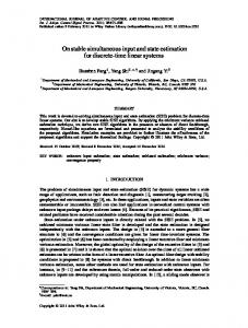
Fault-free case Faulty case

Figure 1: Value of observations.

𝑘→∞

Markov chain we have that Γ(𝑘) 󳨀󳨀󳨀󳨀󳨀→ Γ, 𝐷(𝑘) 󳨀󳨀󳨀󳨀󳨀→ 𝐷, and 𝑘→∞

𝐵(𝑘) 󳨀󳨀󳨀󳨀󳨀→ 𝐵 exponentially fast. From 𝑟𝜎 (𝐴+ √𝜂T(𝑃)𝐶) < 1 and same reasoning as in the proof of proposition 3.36 in [35] we have that 𝑃(𝑘) → 𝑃 as 𝑘 → ∞, where 𝑃 satisfies

+ Ψ (Γ) + 𝐵𝑄𝐵𝑇 + 𝜂T (𝑃) 𝐷𝑅𝐷𝑇 T(𝑃)𝑇 .

350

(65)

And 𝑃 is the unique solution to (65). Recalling that 𝑃 satisfies (62), we get that 𝑃 is also a solution to (65) and from uniqueness, 𝑃̄ = 𝑃. Then, we obtain that ̃ (𝑘 | 𝑘 − 1) ≤ 𝑃. 𝑍

400

(66)

Mean square of residual

̄ + √𝜂T (𝑃) 𝐶)𝑇 𝑃̄ = (𝐴 + √𝜂T (𝑃) 𝐶) 𝑃(𝐴

450

300 250 200 150 100 50 0

And 𝑃(𝑘) → 𝑃. From (66) and (56) in Lemma 10 it follows that 0 ≤ Υ(𝑘) ≤ Υ(𝑘 + 1) ≤ 𝑃(𝑘 + 1 + 𝜅). And thus we can conclude that Υ(𝑘) → Υ whenever 𝑘 → ∞ 𝑘→∞

for some Υ ≥ 0. Moreover, from the fact that 𝛼𝑖 (𝑘) 󳨀󳨀󳨀󳨀󳨀→ 𝜇𝑖 𝑘→∞ ̄ and Γ(𝑘) 󳨀󳨀󳨀󳨀󳨀→ Γ, we have that Υ satisfies (60). From uniqueness of the positive-semidefinite solution to (60), we can conclude that Υ = 𝑃. From (66) and (56), Υ(𝑘) ≤ ̃ + 𝜅 | 𝑘 + 𝜅 − 1) ≤ 𝑃(𝑘 + 𝜅) and since Υ(𝑘) → 𝑃 and 𝑍(𝑘 𝑘→∞ ̃ | 𝑘 − 1) 󳨀󳨀 𝑃(𝑘) → 𝑃 as 𝑘 → ∞, we get that 𝑍(𝑘 󳨀󳨀󳨀→ 𝑃.

The upper bound 𝑃 for the error covariance matrix to a stationary value for linear minimum mean square error (LMMSE) estimation can be easily obtained. It is described that if the system is MSS and the missing information is detected, then the error covariance matrix will converge to the unique nonnegative definite solution of an algebraic Riccati equation associated with the problem.

0

50

100

150

200

250

300

350

400

450

500

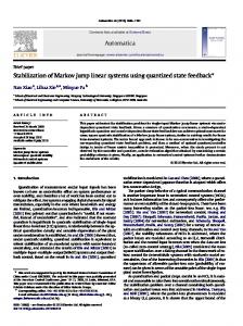
Simulation instant k The corresponding threshold

Figure 2: Mean square of residual.

5. Numerical Example In order to evaluate the performance of our method, in this section, we are going to use a scalar MJLS described by the following equations:

𝑥𝑘+1 = 𝐴 𝑟𝑘 𝑥𝑘 + 𝐵𝑟𝑘 (𝑎𝑟𝑘 + 𝑤𝑘 ) 𝑦𝑘 = 𝛾𝑘 𝐶𝑟𝑘 𝑥𝑘 + 𝐷𝑟𝑘 V𝑘 1 0.995 𝐴1 = ( ), 0 1

1 0.99 𝐴2 = ( ), 0 1

9

2

20

1.8

19

1.6

18

1.4

17

1.2

16

Value of x

Lost information

Abstract and Applied Analysis

1 0.8

15 14

0.6

13

0.4

12

0.2

11

0

10

0

50

100

150

200 250 300 350 Simulation instant k

400

450

500

Real lost informatio Detected value of lost information

17 16.95 16.9 142 144 146 148 0

50

100

150

200 250 300 350 Simulation instant k

400

450

500

Fault-free case Faulty case True x

Figure 3: Detection of fault.

Figure 5: Comparison between state estimators of 𝑥(1) under no faulty case and faulty case, respectively, and real state value.

Average RMS errors of velocity

0.056

covariance of 0.12 , and 𝜇01 = 𝜇02 = 0.5. The transition probability matrix for the finite-state Markov chain is

0.054 0.052

0.6 0.4 Π=( ), 0.4 0.6

0.05

𝑃 (𝛾𝑘 = 1) = 0.9,

0.048

𝑃 (𝛾𝑘 = 0) = 0.1.

To assess the performance of algorithms, the average root mean square (RMS) error based on 𝐻 times Monte-Carlo simulation is defined as

0.046 0.044

(68)

0

5

10

15

20

25

30

35

40

45

50

RMS =

Simulation number FDI-LMMSE LMMSE

Figure 4: Average RMS target position error.

0.1 𝐵1 = 𝐵2 = ( ) , 0 5 𝐷1 = 𝐷2 = ( ) , 0

1 𝐶1 = 𝐶2 = ( ) , 0 𝑎1 = 1,

𝑎2 = 2, (67)

where 𝑥𝑘 (1, 1), 𝑥𝑘 (2, 1), and 𝑎𝑘 denote the target position, velocity, and acceleration, respectively. The initial state 𝑥0 is normally distributed with mean 10 and variance 1. 𝑟𝑘 ∈ {1, 2}, and 𝑤𝑘 , V𝑘 are independent white noise sequences with

2 1/2 1 1 𝐻 𝑇 ∑ ∑ [(𝑥𝑘𝑖 − 𝑥̂𝑘𝑖 ) ] , 𝐻 𝑇 𝑖=1 𝑘=1

(69)

where the time step 𝑇 is chosen as 500, 𝐻 = 50. The simulation results are obtained as follows. Figure 5 presents the real states and their estimators subject to faultfree case and faulty case, respectively, based on the given path. Figure 1 shows the observations with lost data from unreliable channel and observations from reliable channel. As the proposed algorithm can be thought of as a generalization of the well-known LMMSE filtering, we denote it by FDILMMSE filtering in the simulation. The RMS in the position of FDI-LMMSE filtering in the faulty case is compared with that of LMMSE filtering in the fault-free case in the Figure 4. It can be shown in Figures 2 and 3 that the residual can deliver fault alarms soon after the fault occurs. From the simulation results, we can see that the obtained linear estimator for systems with random missing data are tracking well to the real state value, which is the estimation scheme proposed in this paper produces good performance.

10

6. Conclusions This paper has addressed the estimation problem for MJLSs with random missing data. Random missing data introduced by the network is modeled as Bernoulli distribution variable. By usage of an observer-based FDI as a residual generator, the design of FDI-LMMSE filter has been formulated in the framework of LMMSE filtering. Complete analytical solution has been obtained by solving the recursive Riccati equations. It has been proved from theorem derivation and a numerical example simulation that the proposed state estimator is effective.

Conflict of Interests The authors declare that there is no conflict of interests regarding the publication of this paper.

Acknowledgments This work was partially supported by the National Natural Science Foundation of China 61273087 and the Program for Excellent Innovative Team of Jiangsu Higher Education Institutions.

References [1] N. O. Maget, G. Hetreux, J. M. L. Lann, and M. V. L. Lann, “Model-based fault diagnosis for hybrid systems: application on chemical processes,” Computers & Chemical Engineering, vol. 33, no. 10, pp. 1617–1630, 2009. [2] A. Logothetis and V. Krishnamurthy, “Expectation maximization algorithms for MAP estimation of jump Markov linear systems,” IEEE Transactions on Signal Processing, vol. 47, no. 8, pp. 2139–2156, 1999. [3] Y. Bar-Shalom and L. Xiao-Rong, Estimation and Tracking: Principles, Techniques, and Software, Artech House, Norwell, Mass, USA, 1993. [4] G. Ackerson and K. S. Fu, “On state estimation in switching environments,” IEEE Transactions on Automatic Control, vol. 15, no. 1, pp. 10–17, 1970. [5] J. K. Tugnait, “Adaptive estimation and identification for discrete systems with Markov jump parameters,” IEEE Transactions on Automatic Control, vol. 27, no. 5, pp. 1054–1065, 1982. [6] H. A. P. Blom and Y. Bar-Shalom, “Interacting multiple model algorithm for systems with Markovian switching coefficients,” IEEE Transactions on Automatic Control, vol. 33, no. 8, pp. 780– 783, 1988. [7] A. Doucet, N. J. Gordon, and V. Krishnamurthy, “Particle filters for state estimation of jump Markov linear systems,” IEEE Transactions on Signal Processing, vol. 49, no. 3, pp. 613–624, 2001. [8] A. Doucet, A. Logothetis, and V. Krishnamurthy, “Stochastic sampling algorithms for state estimation of jump Markov linear systems,” IEEE Transactions on Automatic Control, vol. 45, no. 2, pp. 188–202, 2000. [9] O. L. V. Costa, “Linear minimum mean square error estimation for discrete-time Markovian jump linear systems,” IEEE Transactions on Automatic Control, vol. 39, no. 8, pp. 1685–1689, 1994.

Abstract and Applied Analysis [10] O. L. V. Costa and S. Guerra, “Stationary filter for linear minimum mean square error estimator of discrete-time Markovian jump systems,” IEEE Transactions on Automatic Control, vol. 47, no. 8, pp. 1351–1356, 2002. [11] L. A. Johnston and V. Krishnamurthy, “An improvement to the interacting multiple model (IMM) algorithm,” IEEE Transactions on Signal Processing, vol. 49, no. 12, pp. 2909–2923, 2001. [12] Q. Zhang, “Optimal filtering of discrete-time hybrid systems,” Journal of Optimization Theory and Applications, vol. 100, no. 1, pp. 123–144, 1999. [13] N. E. Nahi, “Optimal recursive estimation with uncertain observation,” IEEE Transactions on Information Theory, vol. 15, no. 4, pp. 457–462, 1969. [14] Z. Hui, S. Yang, and A. S. Mehr, “Robust energy-to-peak filtering for networked systems with time-varying delays and randomly missing data,” IET Control Theory & Applications, vol. 4, no. 12, pp. 2921–2936, 2010. [15] S. Jun and H. Shuping, “Nonfragile robust finite-time 𝐿 2 -𝐿 ∞ controller design for a class of uncertain Lipschitz nonlinear systems with time-delays,” Abstract and Applied Analysis, vol. 2013, Article ID 265473, 9 pages, 2013. [16] Z. Hui, W. Junmin, and S. Yang, “Robust 𝐻∞ sliding-mode control for Markovian jump systems subject to intermittent observations and partially known transition probabilities,” Systems & Control Letters, vol. 62, no. 12, pp. 1114–1124, 2013. [17] Z. Hui, S. Yang, and L. Mingxi, “𝐻∞ step tracking control for networked discrete-time nonlinear systems with integral and predictive actions,” IEEE Transaction on Industrial Informations, vol. 9, no. 1, pp. 337–345, 2013. [18] H. Shuping, S. Jun, and L. Fei, “Unbiased estimation of Markov jump systems with distributed delays,” Signal Processing, vol. 100, pp. 85–92, 2014. [19] H. Shuping, “Resilient 𝐿 2 -𝐿 ∞ filtering of uncertain Markovian jumping systems within the finite-time interval,” Abstract and Applied Analysis, vol. 2013, Article ID 791296, 7 pages, 2013. [20] H. Shuping and L. Fei, “Robust finite-time estimation of Markovian jumping systems with bounded transition probabilities,” Applied Mathematics and Computation, vol. 222, pp. 297–306, 2013. [21] H. Shuping and L. Fei, “Finite-time 𝐻∞ fuzzy control of nonlinear jump systems with time delays via dynamic observer-based state feedback,” IEEE Transactions on Fuzzy Systems, vol. 20, no. 4, pp. 605–613, 2012. [22] M. Yilin and B. Sinopoli, “Kalman filtering with intermittent observations: tail distribution and critical value,” IEEE Transactions on Automatic Control, vol. 57, no. 3, pp. 677–689, 2012. [23] E. Cinquemani and M. Micheli, “State estimation in stochastic hybrid systems with sparse observations,” IEEE Transactions on Automatic Control, vol. 51, no. 8, pp. 1337–1342, 2006. [24] S. C. Smith and P. Seiler, “Estimation with lossy measurements: jump estimators for jump systems,” IEEE Transactions on Automatic Control, vol. 48, no. 12, pp. 2163–2171, 2003. [25] B. Sinopoli, L. Schenato, M. Franceschetti, K. Poolla, M. I. Jordan, and S. S. Sastry, “Kalman filtering with intermittent observations,” IEEE Transactions on Automatic Control, vol. 49, no. 9, pp. 1453–1464, 2004. [26] C. E. DeSouza and M. D. Fragoso, “𝐻∞ filtering for Markovian jump linear systems,” International Journal of Systems Science, vol. 33, no. 11, pp. 909–915, 2002. [27] C. E. DeSouza and M. D. Fragoso, “Robust 𝐻∞ filtering for uncertain Markovian jump linear systems,” International

Abstract and Applied Analysis

[28]

[29]

[30]

[31]

[32]

[33]

[34]

[35]

[36]

[37]

[38]

[39]

Journal of Robust and Nonlinear Control, vol. 12, no. 5, pp. 435– 446, 2002. Z. Hui, S. Yang, and S. M. Aryan, “Robust weighted 𝐻∞ filtering for networked systems with intermittent measurements of multiple sensors,” International Journal of Adaptive Control and Signal Processing, vol. 25, no. 4, pp. 313–330, 2011. S. M. K. Mohamed and S. Nahavandi, “Robust filtering for uncertain discrete-time systems with uncertain noise covariance and uncertain observations,” in Proceedings of the 6th IEEE International Conference on Industrial Informatics (IEEE INDIN ’08), pp. 667–672, Daejeon, Republic of Korea, July 2008. S. M. K. Mohamed and S. Nahavandi, “Robust finite-horizon Kalman filtering for uncertain discrete-time systems,” IEEE Transactions on Automatic Control, vol. 57, no. 6, pp. 1548–1552, 2012. L. Wenling, J. Yingmin, D. Junping, and Z. Jun, “Robust state estimation for jump Markov linear systems with missing measurements,” Journal of the Franklin Institute, vol. 350, no. 6, pp. 1476–1487, 2013. L. Yueyang, Z. Maiying, and Y. Shuai, “On designing fault detection filter for discrete-time nonlinear Markovian jump systems with missing measurements,” in Proceedings of the 31st Chinese Control Conference, pp. 5384–5389, Hefei, China, 2012. C. Han and H. Zhang, “Optimal state estimation for discretetime systems with random observation delays,” Acta Automatica Sinica, vol. 35, no. 11, pp. 1446–1451, 2009. H. Shuping and L. Fei, “Adaptive observer-based fault estimation for stochastic Markovian jumping systems,” Abstract and Applied Analysis, vol. 2012, Article ID 176419, 11 pages, 2012. O. L. V. Costa, M. D. Fragoso, and R. P. Marques, Discrete-Time Markov Jump Linear Systems, Springer, New York, NY, USA, 2005. U. Orguner and M. Demirekler, “An online sequential algorithm for the estimation of transition probabilities for jump Markov linear systems,” Automatica, vol. 42, no. 10, pp. 1735–1744, 2006. O. L. V. Costa and M. D. Fragoso, “Stability results for discretetime linear systems with Markovian jumping parameters,” Journal of Mathematical Analysis and Applications, vol. 179, no. 1, pp. 154–178, 1993. O. L. V. Costa and S. Guerra, “Stationary filter for linear minimum mean square error estimator of discrete-time Markovian jump systems,” IEEE Transactions on Automatic Control, vol. 47, no. 8, pp. 1351–1356, 2002. M. H. A. Davis and R. B. Vinter, Stochastic Modelling and Control, Monographs on Statistics and Applied Probability, Chapman & Hall, New York, NY, USA, 1985.

11

Advances in

Operations Research Hindawi Publishing Corporation http://www.hindawi.com

Volume 2014

Advances in

Decision Sciences Hindawi Publishing Corporation http://www.hindawi.com

Volume 2014

Journal of

Applied Mathematics

Algebra

Hindawi Publishing Corporation http://www.hindawi.com

Hindawi Publishing Corporation http://www.hindawi.com

Volume 2014

Journal of

Probability and Statistics Volume 2014

The Scientific World Journal Hindawi Publishing Corporation http://www.hindawi.com

Hindawi Publishing Corporation http://www.hindawi.com

Volume 2014

International Journal of

Differential Equations Hindawi Publishing Corporation http://www.hindawi.com

Volume 2014

Volume 2014

Submit your manuscripts at http://www.hindawi.com International Journal of

Advances in

Combinatorics Hindawi Publishing Corporation http://www.hindawi.com

Mathematical Physics Hindawi Publishing Corporation http://www.hindawi.com

Volume 2014

Journal of

Complex Analysis Hindawi Publishing Corporation http://www.hindawi.com

Volume 2014

International Journal of Mathematics and Mathematical Sciences

Mathematical Problems in Engineering

Journal of

Mathematics Hindawi Publishing Corporation http://www.hindawi.com

Volume 2014

Hindawi Publishing Corporation http://www.hindawi.com

Volume 2014

Volume 2014

Hindawi Publishing Corporation http://www.hindawi.com

Volume 2014

Discrete Mathematics

Journal of

Volume 2014

Hindawi Publishing Corporation http://www.hindawi.com

Discrete Dynamics in Nature and Society

Journal of

Function Spaces Hindawi Publishing Corporation http://www.hindawi.com

Abstract and Applied Analysis

Volume 2014

Hindawi Publishing Corporation http://www.hindawi.com

Volume 2014

Hindawi Publishing Corporation http://www.hindawi.com

Volume 2014

International Journal of

Journal of

Stochastic Analysis

Optimization

Hindawi Publishing Corporation http://www.hindawi.com

Hindawi Publishing Corporation http://www.hindawi.com

Volume 2014

Volume 2014