International Journal of Information Technology and Knowledge Management January-June 2012, Volume 5, No. 1, pp. 195-200
INTERVAL TYPE-2 FUZZY SYSTEM FOR AUTONOMOUS NAVIGATIONAL CONTROL OF NON-HOLONOMIC VEHICLES Satvir Singh Sidhu1, Jasbir Singh Saini2 and Arun Khosla3
ABSTRACT: This paper reports the strategy implementation, in simulation environment, for navigation of non-holonomic vehicles using an Interval Type-2 (IT2) Fuzzy Logic System (FLS). A Graphical User Interface (GUI) in MATLAB has been designed to aid the simulations of navigation starting from any position and orientation in a designated area to a designated parking place and fixed orientation. The FLS takes two inputs, vehicle location and orientation w.r.t. x-axis, to deliver one output, the steering angle, relevant to the steering process. The variables take on linguistic values for invoking the rulebase to deliver decisions to steer the vehicle to reach its final parking position. Linear Path Approximation (LPA) trajectory-traversing algorithms for non-holonomic motions have been integrated into the design of the GUI. The FLS was originally developed using Type-1 Fuzzy Sets (T1 FSs), and then enhanced to IT2 FLS by making use of IT2 FSs to handle uncertainties of T1 FLSs. The response of IT2 FLS becomes equivalent to that of T1 FLS as the extent of uncertainty, i.e., Footprint of Uncertainty (FOU) is reduced to zero. However, for restricted FOU within certain bounds, a considerable improvements is observed over the case with zero FOU, i.e., compared to T1 FSs case. Keywords: Type-1 Fuzzy Set, Type-2 Fuzzy Set, Interval Type-2 Fuzzy Set, Fuzzy Logic System, Footprint of Uncertainty, Non-holonomic Vehicle, Autonomous Navigation.
1. INTRODUCTION Majority of robots [1] and commercial vehicles, e.g., cars, trucks, etc., are non-holonomic in nature. A non-holonomic vehicle bears certain kinematical constraints owing to its geometrical features and physical constraints like size, speed, maximum steering angle, etc. It may not be able to change orientation without changing the position and/or may only be able to move in a limited number of directions depending upon orientation of its wheels. Navigation of such a vehicle requires a high degree of expertise and often complex maneuvering to reach at exact or close to exact location with a final orientation, when its initial location and/or orientation is arbitrarily altered. A precise final orientation is always needed in outdoor navigation applications such as precision agriculture, horticulture, gardening, forestry, industrial works, social or civil works, space works, geo-studies and a host of applications of loading/unloading of vehicles. Therefore, it is important to conduct studies on navigational strategies for transforming non-holonomic vehicles into autonomous ones. Freeman [2], presents simulation work of a T1 FLS that automatically backs up a truck to a specified point in a loading-unloading dock. Two input variables, orientation 1
2
3
Department of ECE, SBS College of Engineering & Technology, Ferozepur, Punjab, India, E-mail:
[email protected]. Department of Electrical Engineering, DCRUST Murthal, Sonepat, Haryana, India, E-mail:
[email protected]. Department of ECE, National Institute of Technology, Jalandhar, Punjab, India, E-mail:
[email protected].
and x-coordinate of the vehicle, are considered to generate one output variable, steering angle, to move the vehicle to its final parking position. In the area of trajectory planning, Scheuer et. al. [3] report Continuous-Curvature Path Planner for a car-like robot, that computes the path consisting of straight line segments connected with tangential circular arcs. They also extend their work to Simple Continuous Curvature paths to remove the motion constraint at discontinuities by designing a path comprised of pieces, where each piece is a line segment of a circular arc of maximum curvature. Garcia et. al. [4] report implementation, in simulation environment and hardware, of a zone based FLS for outdoor navigation of a car-like vehicle, where complete maneuvering process is divided into three zones, viz. Approximation, Preparation, and Orientation zone. The FLC uses minimum number of input variables and a set of rules to make decisions, iteratively, for the autonomous steering of the agricultural utilities-based robot to reach its final position and orientation from an initial one. In [5], Zadeh generalizes the concept of ordinary FSs [6], now termed as T1 FSs, to Type-2 (T2) FSs to handle uncertainties involved in T1 FLSs. Mendel et. al. in [7], [8], and [9], extend this concept and explore many aspects of T2 FSs and FLSs. They point out four possible sources of uncertainty present in T1 FLSs: (1) the words that are used in the antecedents and consequents of rules can be uncertain because words mean different things to different people, (2) consequents may have a histogram of values associated with
196
I NTERNATIONAL J OURNAL
OF
I NFORMATI ON T ECHNOLOGY
them, especially when knowledge is extracted from a group of experts, who do not agree at all, (3) measurements that activate a T1 FLS may be noisy and, therefore, uncertain and (4) the data that are used to tune the parameters of a T1 FLS may also be noisy. Consequently, many new terms like Embedded FSs, IT2 FSs, Lower Membership Function (LMF), Upper Membership Function (UMF), Footprint of Uncertainty (FOU), etc. have been identified for proper communication and simplification of the design process of T2 [10] and IT2 [11] FLSs. In Section 2, we give an overview of non-holonomic vehicle and its kinematical equations for trajectory calculations. In Section 3, T2 and IT2 FSs and FLSs are reviewed. In Section 4, we discuss the implementation of fuzzy logic controller for autonomous navigation of nonholonomic vehicles and in Section 5, we present our simulation results. Finally, in Section 6, conclusions and future research agenda are put forth.
2. NON-HOLONOMIC VEHICLE KINEMATICS Non-holonomic vehicle cannot change orientation without altering its position and can move in a limited number of directions depending upon orientation of its wheels. Navigation of such a vehicle requires a high degree of expertise to reach at exact or close to exact location with a fixed orientation from any arbitrarily different initial location and orientation.
AND
K NOW LEDGE M ANAGEMENT
2.1. The Mobile Robot The robot model considered in this paper to simulate the navigational strategy is a car-like four-wheeler nonholonomic vehicle. The navigational space for the vehicle is taken as 200 × 200 square units, which is substantial vis-a-vis the vehicle’s dimensions. The vehicle orientation w.r.t. horizontal axis is Φ, and front tyres angle w.r.t. vehicle orientation is θT, as shown in Fig. 1. The vehicle length (L = 30 units) to width (W = 12:8 units) ratio and maximum steering angle of ± 35° are kept same as for majority of car-like vehicles used in similar simulations [1].
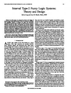
2.2. Trajectory Calculation Module The rear axle mid-point (x, y) has been designated as the reference point of the vehicle for performing the necessary calculations. Robot position is completely specified by three variables, i.e., x, y, and θT (Refer Fig. 1). The trajectory calculation module of FLC determines the vehicle’s next location (x′, y′) and orientation (Φ′), for every displacement per unit time, from the present location (x, y), orientation (Φ) and FLS output, steering angle (θT), as shown in Fig. 2. Calculations involved in this module are based on vehicles kinematical equations are discussed here. This cycle is repeated, based on new vehicle location, orientation, and FLS output steering angle, until the vehicle reaches its final destination. Linear Path Approximation: In this approximation, the front axle mid-point (xa, ya) is subjected to a small linear motion directed by the front tyres angle, as a consequence of which a linear displacement of the rear axle mid-point from (x, y) to (x′, y′) can be seen, as shown in Fig. 1. If the vehicle velocity is v, the distance between front and rear axles is d, and angle of front tyres w.r.t. horizontal axis is γ = Φ + θT, then the LPA algorithmic transformation equations are as follows [12]: Φ′ = Φ + sin–1 [v. sin θT/d]
Figure 1: Linear Path Approximation.
Figure 2: FLC for Navigational Control.
(1)
x′ = x + d. cos Φ + v. cos γ – d. cos Φ′
(2)
y′ = y + d. sin Φ + v. sin γ – d. sin Φ′
(3)
3. TYPE-2 AND INTERVAL TYPE-2 FUZZY SETS AND SYSTEMS Fuzzy logic comprises FSs, a way of representing non-statistical uncertainty and approximate reasoning, and the fuzzy operations used to make inferences. Unlike traditional Aristotelian two-valued logic, in fuzzy logic, belongingness of a variable to a set occurs by a degree over the range [0 1], which is represented by a Membership Function (MF). Type-1 fuzzification is a process of getting one crisp membership grade in [0 1] for every crisp input over the Universe of Discourse (UOD) and the sets are termed as T1 FSs. Such a T1 FS, A, with MF µA(x) is expressed, in fuzzy mathematics, as
I NTERVAL T YPE -2 F UZZY S YSTEM F OR A UTONOMOUS N AVIGATIONAL C ONTROL
A = {(x, µA (x))| ∀ ∈ X}
(4)
A =
or as, A=
[
i
f
,
f
i
]
(5)
where ‘/’ denotes a tuple rather than a division and ‘ ∫ ’ denotes union, over all admissible x, rather than mathematical integration. For discrete universes of discourse, ‘ ∫ ’ is replaced by ‘Σ’.
3.1. Type-2 Fuzzy Sets Most FLSs encode human reasoning into a program to make decisions and/or control a system. However, use of T1 FSs to model words cannot be appreciated as word are uncertain themselves [7-11]. The concept of T2 FSs [5] was initially proposed as an extension of T1 FSs [6] by Lotfi Zadeh as a generalization to the original concept, where the membership grade(s) is(are) not one crisp value for a crisp input over the UOD, but is another single (multiple) T1 FS(s), called secondary MF(s). Such a fuzzification is called general type-2 fuzzification and the sets are called T2 FSs. A T2 FS, , is characterized by a T2 MF, µ ( x, u ), where denoted as A A x ∈ X and u ∈ Jx ⊆ [0, 1], i.e.,
= {(x, u), ( µ A ( x, u ))| ∀ x ∈ X, u ∈ J ⊆ [0, 1]} A x
∫ ∫ x ∈X
u ∈J x
µ A ( x, u ) /( x, u ), J x ⊆ [0,1]
FOU ( A ) =
µ A (x = x′, u) ≡ µ A (x′) =
∫
u ∈J x
in which 0 ≤ fx′ (u) ≤ 1. As ∀ x′ ∈ X, we drop the prime notation on µ A (x′), and refer to µ A (x) as a T1 secondary MF. Based on the concept of secondary sets, we can reinterpret a T2 FS as the union of all secondary T1 FSs, i.e., using (8), in a vertical-slice manner, as we can re-express A
= {x, ( µ A (x)) | ∀ x ∈ X} A
(9)
∫
x ∈X
µ A ( x) / x =
∫
x ∈X
J
x ∈X
...(12)
x
A =
∫ ∫ x ∈X
u ∈J x
1/( x, u ), J x ⊆ [0 1]
(10) The domain of a secondary MF is called the primary membership of x. In (10), Jx is the primary membership of x, where Jx ⊆ [0 1] for all x ∈ X. The amplitude of a secondary MF is called a secondary grade. In (10), fx(u) is a secondary grade. If X and Jx are both discretized into N and Mi values respectively, then the right-most part of (10) can be expressed as
(13)
and (8) reduces to µ A (x = x′, u) ≡ µ A (x′) =
∫
u ∈J x
1/ u ; J x ′ ⊆ [0 1]
(14)
3.3. FOU Representation There are many ways to express FOU [9, 11, 14], and so are
the approaches to describe IT2 FS. FOU of an IT2 FS, say A , can be expressed using only lower and upper bounds of uncertainty involved that are termed as LMF and UMF and are denoted as µ A (x) and µ A (x) respectively, for x ∈ X. Mathematically,
and
µ A (x) = FOU ( A ); x ∈ X
(15)
µ A (x) = FOU ( A ); x ∈ X
(16)
In line with (12), FOU ( A ) =
f (u ) /(u ) / x; J x ⊆ [0,1] ∫u ∈J x x
...(11)
Computational complexities increase exponentially with the number of T2 FSs in an FLS [13]. However, the burden of complexities reduces many folds with a special case of T2 FSs called IT2 FSs, where all secondary MFs of every T2 FS become interval sets (i.e., µ A (x, u) = 1) rather than T1 FSs. Mathematically, from (7), we have
or as,
= A
k =1
(uik ) /(uik ) / xi
3.2. Interval Type-2 Fuzzy Sets
(7)
f x ′ (u ) /(u ); J x ′ ⊆ [0,1] (8)
i =1
xi
The term FOU is very useful, as it not only focuses our attention on the uncertainties inherent in the specific T2 FS, whose shape is a direct consequence of the nature of these uncertainties, but also provides a very convenient verbal description of the entire domain of support for all the secondary grades of a T2 FS.
(6)
Vertical slice of µ A (x, u) at each value of x, say x = x′, the 2D plane whose axes are u and µ A (x′, u), is called secondary MF of µ A (x, u), i.e.,
Mi
∑ ∑ f
197
Uncertainty in the primary memberships of a T2 FS, A , consists of a bounded region called FOU. It is the union of all primary memberships, i.e.,
can also in which 0 ≤ µ A (x, u) ≤ 1 and, alternatively, A be expressed as = A
N
N ON -H OLONOMIC V EHICLES
OF
x ∈X
x ∈X
J x and FOU ( A ) =
J x, where J x and J x denote the lower and upper
bounds on Jx, respectively. Note that if µ A (x) = µ A (x), i.e., all secondary uncertainties disappear, IT2 FS reduces to T1 FS. Stated mathematically,
µ A ( x) |µ A ( x ) = µ A ( x ) = µA(x)
(17)
IT2 FLS has been well standardized in [14] for various operators, defuzzification, and type-reduction methods etc.
198
I NTERNATIONAL J OURNAL
OF
I NFORMATI ON T ECHNOLOGY
3.4. Fuzzy Operators for IT2 FSs Operations of crisp set theory viz. union, intersection and complement, are also applicable in fuzzy set theory. These operations are computationally much easier for the case of IT2 FSs [9, 11] as compared to the case of general T2 FSs [13]. Consider two general T2 FSs A and B over a UOD, X. Using Zadeh's Extension Principle [5], the membership grades for the union, intersection and complement of general
∫
b i ∈[ f i H
µ i , f i H G
µ
Gi
]
(1/ b i ); y ∈ Y
(22)
where µ G i (y) and µGi (y) are the lower and upper membership grades of µ Gi (y). Suppose that N out of M rules in the IT2 FLS get fired, where N ≤ M, and the combined output set, µ B ( y ) , is obtained by combining the output consequent FSs, with the help of t-conorms, of all the fired rules. This is expressed mathematically as µ B ( y) =
= 1/[ µ B (x), µ B (x)] have been defined as follows [13]:
N
µ
(23)
B i
i=1
µ A
µ B = 1/[ µ A (x) ∨ µ B (x), µ A (x) ∨ µ B (x)]
(18)
µ A
µ B = 1/[ µ A (x) H µ B (x), µ A (x) H
(19)
¬ µ A = 1/[1 – µ A (x), 1 – µ A (x)]
K NOW LEDGE M ANAGEMENT
µ B i (y) =
T2 FSs A = 1/FOU( A ) = 1/[ µ A (x), µ A(x)] and B = 1/ FOU( B )
µ B (x)]
AND
(20)
Here, H and ∨ denote the t-norm and t-conorm. , and ¬ are referred to as join, meet and negation respectively, to distinguish them from the operators used in T1 FLSs, i.e., union, intersection and complement.
4. FUZZY LOGIC CONTROLLER (FLC) FLS receives two inputs, i.e., vehicle co-ordinate, x, and vehicle orientation, Φ, w.r.t. horizontal axis, to deliver an output steer, θT, (Refer Fig. 2) to direct the vehicle towards the destination. Table 1 lists all T1 FSs for both inputs and an output, while Table 2 lists all possible (35) linguistic fuzzy rules in the form of rule matrix. Usually, in an FLS, words (uncertain) are modeled using T1FSs (certain) and used to specify IF-THEN fuzzy rules. However, in this paper, to handle uncertainties associated with the use of words, we enhanced T1 FSs to IT2 FSs.
3.5. Fuzzy Rulebase Rules are the kernel of every FLS, and may be provided by experts or extracted from numerical data. In either case, rules are expressed as a collection of IF-THEN statements. A multi-input multi-output (MIMO) rulebase can be considered as a group of multi-input single-output (MISO) rulebases; hence, it is sufficient to concentrate on a MISO rulebase [14]. Consider an FLS having p antecedents, x1 ∈ X1, x2 ∈ X2,..., xp ∈ Xp, (denoted as x collectively) and one consequent y ∈ Y. Assume there are M rules and the ith rule has the form: Ri : IF x1 is F1i and x2 is F2i and ... and xp is Fpi THEN y is G ; i = 1, 2, ..., M. i
This rule represents a T2 relation between the input space, X1× X2× ... × Xp, and the output space, Y, of the IT2 FLS. Fki represent the antecedent FSs with associated µ Fki(xk) MFs (k = 1, 2,…,p) and Gi represents consequent FS of ith rule with associated MF µ G i(y). For a crisp input vector, i.e., x = x′, to an IT2 FLS, The result of the input and antecedent operations, is an IT1 set, called firing set, i.e.,
(a) Crisp inputs location along horizontal axis (x) and vehicle angle w.r.t. horizontal axis (Φ) are fuzzified using T1 FSs initially, and then the FSs of input Φ only are enhanced to IT2 FSs. (b) Calculate the firing interval using fuzzy t-norms (MIN or PRODUCT) on LMF and UMF. (c) Fuzzy rules are fired twice for each single crisp input, firstly, for LMF and secondly, for UMF that leads to two level clipping of output T1 consequent FSs, as shown by dark black shaded regions in Fig. 3 for two fired rules. (d) Resultant output FS, for all fired rules, is aggregated by using MAX operator (t-conorm). Table 1 Fuzzy Sets for Input and Output Variables [12] Fuzyy Input # 1 = x (Co-ordinate) Name
i i i i Fi(x′) = [ f ( x ′ ) , f ( x ′ )] º [ f , f ]
= [ µ F1 ( x′1 )H ...H
4.1. Algorithmic Flow
(21)
µ Fp ( x′p ), µ F1 ( x ′1 )H ...H
µ Fp ( x′ p ) ] The ith rule, Ri, fired output consequent set, µBi(y), is an IT2 FS:
Range
MF Type
[0 0 20 70]
Trapezoidal
LV (Left Vertical)
[60 80 100]
Triangular
VE (Vertical)
[90 100 110]
Triangular
LE (Left)
RV(Right Vertical) RI (Right)
[100 120 140]
Triangular
[130 180 200 200]
Trapezoidal Contd.
I NTERVAL T YPE -2 F UZZY S YSTEM F OR A UTONOMOUS N AVIGATIONAL C ONTROL Fuzyy Input # 2 = (Orientation) Name LB (Left) LU (Left Upper) LV (Left Vertical) VE (Vertical) RV (Right Vertical) RU (Right Upper) RB (Right Below)
Range
MF Type
[170 225 280] [120 155 190] [ 90 112.5 135] [ 80 90 100] [ 45 67.5 90] [ –10 35 60] [–100 –45 10]
Triangular Triangular Triangular Triangular Triangular Triangular Triangular
Fuzyy Output # 1 = (Steer) Name
Range
MF Type
NB (Negative Big) [–35 – 35 – 17] NM (Negative Medium) [–30, – 17, –7] NS (Negative Small) [ –14, – 7 0] ZE (Zero) [ –7, 0 7] PS (Positive Small) [0 7 14] PS (Positive Medium) [7 17 30] PB (Positive Big) [17 35 35]
Triangular Triangular Triangular Triangular Triangular Triangular Triangular
OF
N ON -H OLONOMIC V EHICLES
199
(f) Here, crisp output θT is computed as mean of both centroids [θTL, θTR]. Mathematically, θT = mean (θTL, θTR)
(24)
5. SIMULATION RESULTS A screen snap shot of the designed GUI, for navigation of non-holonomic autonomous vehicle, is shown in Fig. 4. Navigational space of 200 × 200 square units is provided to see the traces of the vehicle when simulated. Simulations can be performed in customized display by selecting no trails, trailing front tyres, trailing rear tyres or trailing vehicle’s boundary, etc. The following are the observations derived from mobile robot navigation simulations: (a) The t-norms MIN or PRODUCT do not create much difference, however, from detailed analysis tabulated in Table 3, it can be observed that MSE or RMSE with MIN t-norm is lesser than that of PRODUCT t-norm in both T1 and IT2 FLSs.
Table 2 Rule Set for Autonomous Vehicle Navigation [12] x (Location) F (Orientation) RB RU RV VE LV LU LB
LE
LV
VE
RV
RI
PS NS NM NM NB NB NB
PM NM PS NS NM NB NB
PM PM PS ZE NS NM NM
PB PB PM PM PS NS NM
PB PB PB PM PM PS NS
Figure 4: Vehicle Traces with Different Locations, Orientation and FOUs in Vehicle Angles in GUI Based Simulation Environment.
(b) Simulations for navigation of non-holonomic four wheeled vehicle are carried out from seven locations tabulated in Table 3, distributed all around the designated area, with initial vehicle angles 0° and 180° and with FOU in vehicle angle, Φ, equal to 0 and 3. Figure 3: Rule Firing on IT2 FLS.
(e) Centroids θTL and θTR for each of aggregated LMF and UMF is then computed as:
∑ = ∑
N
θTL
y µ B ( yi )
i =1 i N i =1
µ B ( yi )
∑ ∑
N
and θTR =
y µ B ( yi )
i =1 i N i =1
µ B ( yi )
(c) FOU, if introduced, in vehicle location, x, and/or steering angle, θT, shows little improvements. The reason is very small contribution in calculation of next location of the vehicle as observed from kinematic equations discussed in Section 2.2. (d) The response of the IT2 FLS, with FOU 3 in Φ, has been found to be better than that of T1 FLS, when FOU is 0. Firstly, from visual analysis (Refer Fig. 4)
200
I NTERNATIONAL J OURNAL
OF
I NFORMATI ON T ECHNOLOGY
one can see that the vehicle is better aligned in IT2 FLS than that in T1 FLS, and secondly the errors MSE or RMSE are comparatively lesser in IT2 than in T1 FLS as shown in Table 3.
K NOW LEDGE M ANAGEMENT
high degree of expertise and maneuvering. However, designing robust FLS for autonomous navigation of nonholonomic vehicles, that can cope up with changing environmental conditions, are still on our future research agenda.
Table 3 Comparison of Two t-norms and FOU in
REFERENCES
Detoured From Target S. No. Vehicle Angle
AND
X
Y
IT2 (FOU = 3) T1(FOU = 0) Min Prod Min Prod
1
0
20
50
–0.3
–1.1
– 3.1
– 3.1
2
0
20
100
0.8
–0.1
–6.6
–7.0
3
0
20
150
–8.6
–10.6
–15.6
–16.8
4
0
100
40
–0.9
–1.4
–0.1
–1.0
5
0
180
50
–0.9
–0.4
1.3
1.8
6
0
180
100
0.5
1.9
5.8
5.8
7*
0
180
150
21.1
21.8
16.6
16.5
8
180
20
50
0.1
–0.3
–3.7
–3.5
9
180
20
100
–2.8
–3.2
–7.9
–7.9
10*
180
20
150
–23.3
–22.7
–18.5
–18.4
11
180
100
40
–0.8
–0.7
1.0
–1.0
12
180
180
50
–0.8
–1.3
1.1
1.4
13
180
180
100
–0.4
0.1
4.7
5.2
14
180
180
150
8.0
9.2
14.6
15.0
MSE
81.28
86.21
90.23
94.23
RMSE
9.02
9.29
9.50
9.71
(e) In Table 3, S. Nos. 7 and 10 are '*'-marked to highlight the poor performance of IT2 FLS than that of T1 FLS as vertical room left for steering the vehicle is not sufficient for IT2 FSs. However, it was seen that as FOU in Φ is decreased with increasing y-coordinate, the parking performance of the vehicle again improves.
6. CONCLUSIONS AND FURTHER SCOPE We have proposed designing of FLS for better navigational strategy for non-holonomic vehicles, where vehicle orientation, ?, has been fuzzified using IT2 FSs. Use of MIN as t-norm operator further increases the accuracy of the vehicle reaching at the designated parking location. This paper explores some strategic aspects (e.g., choice of t-norm operators and amount of FOU in vehicle orientation) in simulation environment for autonomous control of non-holonomic vehicles that otherwise requires
[1]
L. Garcia-Perez, M. Garcia-Alegre, “A Simulation Environment to Test Fuzzy Navigation Strategies Based on Perceptions”, In: IEEE International Conference on Fuzzy Systems, 2, pp. 590-593, 2001.
[2]
J. A. Freeman, “Fuzzy Systems for Control Applications: The Truck Backer-Upper”, The Mathematica Journal: Artificial Intelligence, 4 (1), pp. 64-69, 1994.
[3]
A. Scheuer, T. Fraichard, “Planning Continuous-Curvature Paths for Car Like Robots”, In: IEEE/RSJ International Conference on Intelligent Robots and Systems, 3, Osaka, Japan, pp.1304-1311, 1996.
[4]
L. Garcia-Perez, M. Garcia-Alegre, A. Ribeiro, D. Guinea, “A Simulation Environment to Test Fuzzy Navigation Strategies Based on Perceptions”, In: IV Workshop on Physical Agents, Alicance, Spain, pp. 87-98, 2003.
[5]
L. A. Zadeh, “The Concept of a Linguistic Variable and Its Application to Approximate Reasoning-1”, Information Sciences, 8, pp. 199-249, 1975.
[6]
L. A. Zadeh, “Fuzzy Sets”, Information and Control, 8, pp. 338-353, 1965.
[7]
N. N. Karnik, J. M. Mendel, L. Qilian, “Type-2 Fuzzy Logic Systems”, IEEE Transactions on Fuzzy Systems, 7(6), pp. 643-658, 1999.
[8]
J. M. Mendel, Uncertainty, “Fuzzy Logic, and Signal Processing”, Signal Processing, 80 (6), pp. 913-933, 2000.
[9]
Q. Liang, J. M. Mendel, “Interval Type-2 Fuzzy Logic Systems: Theory and Design”, IEEE Transactions on Fuzzy Systems, 8(5), pp. 535-550, 2000.
[10] J. M. Mendel, R. I. John, “Type-2 Fuzzy Sets Made Simple”, IEEE Transactions on Fuzzy Systems, 10(2), pp. 117-127, 2002. [11] J. M. Mendel, R. I. John, F. Liu, “Interval Type-2 Fuzzy Logic Systems Made Simple”, IEEE Transactions on Fuzzy Systems, 14(6), pp. 808-821, 2006. [12] V. Mutneja, S. Singh, N. Gill, J. S. Saini, “Mobile Robot Navigation using IT2-FLS, IEEE National Conference on Applications of Intelligent Systems”, Sonepat, India, pp.18-23, 2008. [13] N. N. Karnik, J. M. Mendel, “Operations on Type-2 Fuzzy Sets”, International Journal on Fuzzy Sets & Systems, 122, pp. 327-348, 2001. [14] J. M. Mendel, “Advances in Type-2 Fuzzy Sets and Systems”, Information Sciences, 177, pp. 84-110, 2007.