Inverse Parameter Estimation using Hamilton-Jacobi ... - KTH DiVA

Inverse Parameter Estimation using Hamilton-Jacobi Equations

MIKAEL

HELIN

Master of Science Thesis Stockholm, Sweden 2013

Inverse Parameter Estimation using Hamilton-Jacobi Equations

MIKAEL

HELIN

2D1020, Master’s Thesis in Numerical Analysis (30 ECTS credits) Degree Progr. in Engineering Physics 270 credits Royal Institute of Technology year 2013

Supervisor at KTH was Anders Szepessy Examiner was Michael Hanke TRITA-MAT-E 2013:26 ISRN-KTH/MAT/E--13/26--SE

Royal Institute of Technology School of Engineering Sciences KTH SCI SE-100 44 Stockholm, Sweden URL: www.kth.se/sci

Abstract In this degree project, a solution on a coarse grid is recovered by fitting a partial differential equation to a few known data points. The PDE to consider is the heat equation and the Dupire’s equation with their synthetic data, including synthetic data from the Black-Scholes formula. The approach to fit a PDE is by optimal control to derive discrete approximations to regularized Hamilton characteristic equations to which discrete stepping schemes, and parameters for smoothness, are examined. By non-parametric numerical implementation the dervied method is tested and then a few suggestions on possible improvements are given. Keywords: Hamilton-Jacobi equation. Optimal control. Euler method.

Referat Inversa parameteruppskattningar genom tillämpning av Hamilton-Jacobi ekvationer I detta examensarbete återskapas en lösning på ett glest rutnät genom att anpassa en partiell differentialekvation till några givna datapunkter. De partiella differentialekvationer med deras motsvarande syntetiska data som betraktas är värmeledningsekvationen och Dupires ekvation inklusive syntetiska data från BlackScholes formel. Tillvägagångssättet att anpassa en PDE är att med hjälp av optimal styrning härleda diskreta approximationer på ett system av regulariserade Hamilton karakteristiska ekvationer till vilka olika diskreta stegmetoder och parametrar för släthet undersöks. Med en icke-parametrisk numerisk implementation prövas den härledda metoden och slutligen föreslås möjliga förbättringar till metoden. Nyckelord: Hamilton-Jacobi ekvationer. Optimal styrning. Eulers stegmetoder.

Contents I Introduction with Basic Theory

1

1 Notation and Introduction 1.1 Overview . . . . . . . . . . . . . . . . . . . . . . . . . . . . . . 1.1.1 The Model Problem . . . . . . . . . . . . . . . . . . . 1.1.2 The Finance Problem . . . . . . . . . . . . . . . . . . . 1.2 Notation . . . . . . . . . . . . . . . . . . . . . . . . . . . . . . 1.2.1 The Column Vector Convention, Elementwise Multiplication and the Vector Valued Function with its Jacobian 1.2.2 Notation for Discretization and Approximation . . . . 1.2.3 Train of Pulses . . . . . . . . . . . . . . . . . . . . . . 1.2.4 Notation for Differential Equations and their Approximations . . . . . . . . . . . . . . . . . . . . . . . . . . 1.2.5 Notation for Stepping Schemes and a Modified Midpoint Method . . . . . . . . . . . . . . . . . . . . . . . . . . 1.2.6 Some Additional Notation . . . . . . . . . . . . . . . .

3 3 5 7 10 10 11 12 13 14 17

2 Creating Synthetic Data 2.1 Choosing a Continuous Solution to the Model Problem . . . . 2.1.1 A First Simple Application . . . . . . . . . . . . . . . . 2.2 Choosing Discrete Synthetic Data to the Model Problem . . . 2.2.1 Discrete Representations of the Model Problem . . . . 2.2.2 Comparison of Different Synthetic Data and Experiments with Noisy Heat Conductivity . . . . . . . . . . 2.3 Choosing Synthetic Data to the Finance Problem . . . . . . . 2.4 Von Neumann Stability Analysis . . . . . . . . . . . . . . . . .

21 22 23 25 25

3 Optimal control 3.1 Definitions . . . . . . . . . . . . 3.2 The Hamilton-Jacobi Equation 3.3 Lipschitz Continuity . . . . . . 3.4 The Hamilton Characteristics .

49 49 51 52 54

. . . .

. . . .

. . . .

. . . .

. . . .

. . . .

. . . .

. . . .

. . . .

. . . .

. . . .

. . . .

. . . .

. . . .

. . . .

. . . .

. . . .

32 37 44

3.4.1 3.4.2 3.4.3

3.5

Method by Lagrange . . . . . . . . . . . . . . . . . . . Some Property of the Optimal Control . . . . . . . . . Obtaining the Hamilton-Jacobi-Bellman Equation by Continuous Time Dynamic Programming . . . . . . . . . . 3.4.4 Deriving the Characteristic Equations to the HamiltonJacobi Equation . . . . . . . . . . . . . . . . . . . . . . 3.4.5 Deriving the Value Function from the Hamilton-JacobiBellman Equation . . . . . . . . . . . . . . . . . . . . . 3.4.6 The Pontryagin Principle with an Application . . . . . Additional Comments to Optimal Control . . . . . . . . . . .

II Application with Results

54 55 56 59 60 61 64

65

4 Solving the Model Problem 67 4.1 Deriving the Hamilton Characteristic Equations . . . . . . . . 68 4.1.1 A Continuous Approach in Deriving Characteristic Equations . . . . . . . . . . . . . . . . . . . . . . . . . . . . 69 4.1.2 Choosing the Optimal Control . . . . . . . . . . . . . . 73 4.1.3 Regularizing the Optimal Cost Function . . . . . . . . 75 4.1.4 Solving the Hamilton Characteristics . . . . . . . . . . 79 4.1.5 The Hamilton-Jacobi Characteristic Equations From the Discrete Approximation to the Model Problem . . . . . 82 4.2 The Results . . . . . . . . . . . . . . . . . . . . . . . . . . . . 84 4.2.1 A Minimal Description of the Solving Algorithm . . . . 84 4.2.2 Testing with a Coarse Grid . . . . . . . . . . . . . . . 86 4.2.3 Synthetic Solution Given as Start Solution . . . . . . . 93 5 Solving the Finance Problem 97 5.1 Deriving the Hamilton Characteristics . . . . . . . . . . . . . 97 5.1.1 A Suggestion for an Advanced Alternative to the Dupire’s Equation . . . . . . . . . . . . . . . . . . . . . . . . . . 99 5.1.2 A Simple Alternative to the Dupire’s Equation . . . . . 100 5.1.3 The Trice-Ruby Parameters . . . . . . . . . . . . . . . 101 5.2 The Results . . . . . . . . . . . . . . . . . . . . . . . . . . . . 102 5.2.1 Improved Results . . . . . . . . . . . . . . . . . . . . . 108 5.2.2 Recovering Black-Scholes Data with Varying Global Volatility . . . . . . . . . . . . . . . . . . . . . . . . . . . . . 108 5.2.3 The +MH method . . . . . . . . . . . . . . . . . . . . 111 5.2.4 Solving by use of Black-Scholes Formula . . . . . . . . 113

6 Conclusion

119

Bibliography

127

Part I Introduction with Basic Theory

1

Chapter 1 Notation and Introduction 1.1

Overview

We usually think of cause and effect rather than its reverse, effect and its cause. However, it is not uncommon to face situations where one needs to think in reverse manner, i.e. that from ’effect’ try to figure out the ’cause’. To give some clearer picture; imagine a simple problem in ballistics: A forward problem is to figure out the trajectory of a cannon ball given its initial conditions. Forward problems are in general much easier to solve than inverse problems. Opposed to the given forward problem, an inverse problem is when one finds this cannon ball buried into the ground and wants to find out which location the cannon ball was shot from. In this example the ’cause’ is the firing and how the cannon is directed and the ’effect’ is where the ball hits or lands. Another example is how a traveler “thinks forward” when traveling by metro to the art museum. The lost traveler could ask anyone for directions by metro to the art museum and then easily get there. The reverse, if the lost traveler does not remember where he entered the subway system and asks people awkwardly “Where did I enter the subway?” then the task of finding back to point of entry into the subway is harder than the task of traveling to the art museum. The traveler could for example provide information (data), such as he entered the subway 20 minutes ago, and by that information one is able to figure out some handful number of answers. More technically speaking, an inverse problem is when one has some given data and from them tries to find out some parameters, equations or other properties that yield the same data for the corresponding forward problem. When the inverse problem is solved then its result can be used for solving other problems forward provided the parameters are estimated. There are 3

CHAPTER 1. NOTATION AND INTRODUCTION

many benefits where one should solve the inverse problem first. One obvious reason is when some forward problem cannot be solved until its corresponding inverse problem is solved first. Another possible reason is when one wins computing time by solving the inverse problem first before solving any other problems. An analog to won computing time is the time saved when using dynamic programming for solving optimization problems.1 And one could be interested to estimate the parameter space by solving the inverse problem. I will only mention suggestions on how to recover parameters without actually recovering any parameters. In this degree project, I work with the heat equation and the Dupire’s equation to which for some given data points the inverse problem is to recover the remaining unknown data points. And to do this, I use optimal control. Optimal control is a branch of mathematics that is an extension to calculus of variations and developed mostly by the mathematician Pontryagin in the Soviet Union and applied mathematician Bellman from USA. A quick explanation in optimal control is in Chapter 3 where the Hamilton-Jacobi-Bellman equation is derived by use of continuous dynamic programming and then further I explain and derive the HamiltonJacobi characteristic equations (1.6).2 The derivation in Chapter 3 is applied and partially mimicked in chapters 4.1 and 5.1. In Chapter 4.1 I derive and in Chapter 4.2 I numerically solve regularized Hamilton characteristic equations related to the problems dealing with the heat equation explained in Chapter 1.1.1. The title of this degree project is thoroughly explained in the end of Chapter 1.1.1. In Chapter 5.1 I derive and in Chapter 5.2 I numerically solve regularized Hamilton characteristic equations related to the problems dealing with the Dupire’s equation explained in Chapter 1.1.2. A reason for different approaches on deriving characteristic equations is to ensure that the derived characteristic equations are correct. It has shown that issues with convergence for synthetic data is related to the dimensions of its grid as well as it has shown that convergence of the solution is related to the quality of its corresponding synthetic data. Chapter 2 is mainly written in consideration of grid dimensions and quality of synthetic data. The numerical work in this degree project is about a few numerical methods used for solving discrete approximations of the Hamilton characteristic equations. The implementation used is with non-parametric control. Different stepping methods in time, results from smoothness and different grids are tested and evaluated. In the 1

A computational benefit with dynamic programming is that one does not need to compute every possible path to find the optimal solution. A few similar benefits can be obtained by solving inverse problems. 2 The system of equations (1.6) is as well a regularized approximation. The notation for approximations are explained in Chapter 1.2. Regularized means that the equations are manipulated in such way that the problem becomes well-posed in some sense.

4

1.1. OVERVIEW

final chapter, chapter 6, I have my conclusion on solving these approximations of Hamilton characteristic equations. In this degree project, I do not discuss about current technological or mathematical advancements in optimal control but instead give a few ideas of improvement explained in chapter 5.2.1. The work in this degree project, is basically by experimentation to test and verify some of the theory presented in [13],[14],[15].

1.1.1

The Model Problem

To explain things more simple, we need a model problem. Dr. David, a secret scientist at Area 51, wants to study the effects of healing on chronic blood cells by use of light emitting ore. For best effect, Dr. David chooses to have a stick emitting green light, to resemble a lantern, made out of kryptonite. It is well-known that the radiation from the very exotic crystallized metal has marvelous effects on living creatures on earth.3 To be able to conduct the experiment, Dr. David needs help in knowing the heat distribution inside this stick for computing effects of light emission onto his living test subjects. So assume we have a thin rod of kryptonite of length 2 with a heat conductivity that varies both by time and space. The rod has ice on its both ends, such that the temperature at the ends stays constantly at 0◦ C. Denote time by t ∈ [0, 1], space by x ∈ [0, 2] and the heat in the rod by X = X(t, x) ∈ R and let the domain Ω be such that Ω = [0, 1] × [0, 2]. The model equation we use in this text is the one dimensional heat equation of the form Xt − (σXx )x = 0

(1.1)

X(0, x) = g(x)

(1.2)

X(t, 0) = X(t, 2) = 0

(1.3)

with initial condition and boundary conditions

where σ = σ(t, x) is a parameter for heat conductivity such that σ : Ω → [0, ∞) and partial derivatives Xt (t, x) and Xx (t, x) such that Xt (t, x) =

∂ X(t, x) ∂t

Xx (t, x) =

∂ X(t, x). ∂x

and

3

As a reference there are several issues of Marvel comics to attest this fact.

5


To be able to test and examine inverse problems, we need given data, and such data I have chosen to be synthetic rather than real.4 The true data or ˆˆ the true solution which we derive by synthetic means we denote by X. When measuring data from the real world it might include some noise, so sometimes I add noise into the models. The given data or measured data we denote by ˆˆ ˆ Normally, in real world problems X X. is never known and all we have is a ˆ few given samples of X. The first problem, which we call the model problem, is to find the parameter σ : Ω → R such that min σ

Z

Ω

1 ¯ ˆ x)]2 µ(t, x) dx dt = [X(t, x) − X(t, 2 X 1 ¯ a , xb ) − X(t ˆ a , xb ))2 (1.4) = min (X(t k k k k σ 2 ak ,bk

¯ x) solves (1.1)-(1.3) and where µ(t, x) is the sum of impulse funcwhere X(t, tions such that X δ(t − tak , x − xbk ) (1.5) µ(t, x) = ak ,bk

ˆ a , xb ) are known for all given ak and bk . Consider σ as some provided X(t k k control variable, so what we look for is a control σ that minimizes the error in (1.4). A main objective with this degree project is to find a solution to the problem (1.1)-(1.5) and instead of solving (1.1)-(1.5) we solve another easier problem numerically, namely the system of regularized Hamilton characteristic equations5 ¯ x)), ¯ t (t, x) = H ς (X(t, ¯ x), λ(t, X λ (1.6) ς ¯ ¯ x)), ¯ −λt (t, x) = HX (X(t, x), λ(t, and compare the approximate solution by the Hamilton characteristic equations (1.6) to its synthetic solution by measuring the error Z

Ω

1 ¯ ˆ x)]2 µ(t, x) dx dt. [X(t, x) − X(t, 2

Unfortunately, the solution to (1.6) may be very different to the solution to (1.1)-(1.5). Experimentally, another task is to examine the quality of the solution to (1.6) by use of different numerical schemes. Such schemes are forward Euler method, backward Euler method and some other methods used for stepping in time. 4

Since I failed to find some authentic kryptonite for making real measurements I had to synthesize data. 5 The variable ς is a smoothness parameter explained in chapter 4.1.3

6

1.1. OVERVIEW

Opposed to curve fitting a function to its given data, the term calibration is used for fitting the parameters of a PDE to its given data. It was previously mentioned that in this degree project we recover remaining unknown data ¯ from some given data points X. ˆ By solution, I specifically mean the points X ¯ and not the calibrated parameters (or control) ¯ (or X) recovered data points X σ ¯ that minimizes (1.4).

1.1.2

The Finance Problem

Mr. J Timbo at Lake Valiente imports in Gwens Guinea. There will be a rain which is one sun cycle away from now.6 J Timbo needs 59,000 units of logs and

logs from the holy and sacred woods dance festival in the name of Esther, Until then, at the day of Esther, Mr. each unit costs 1C$ (Curtis dollar).

There are different ways Mr. J Timbo can acquire this timber. One way is to buy from Mr. Ramone and pay 59, 000C$ in cash and then keep the timber at the lake for a sun cycle. But if Mr. J Timbo buys the logs now, his capital is tied up for a full cycle. Another idea is to wait a full sun cycle and then purchase the logs, but then the drawback is that the market price of the logs may change. One reason why the price of the logs changes depends on the loved woodpeckers Nikki and Keririh. It is considered that when Nikki and Keririh drum holes into the trees, the value of the pecked timber increase since the characteristic markings in the logs is the trademark logo for the brand of “export quality logs from Gwens Guinea”. Depending on how active Nikki and Keririh are among a few other factors, such as storms and rains, decide the market price for logs. It is possible to estimate the drumming activity of Nikki and Keririh but to forecast storms and effects of storms (that cut logs in an orderly or messy way) is harder to predict.7 A brilliant idea is to buy an European call option for the price C from Mr. J Lloyd at the local bank. To see the definition of European call options, which in short are just called European calls, they can be found in [1], [2], [9], [13], [16], [17]. By far the best text in financial mathematics that I know of is [1]. 6

To us who believe the earth revolves around the sun a sun cycle is equivalent to a year. A sun cycle is not to be confused with the day cycle of evening and morning as described in Genesis 1:3-5. 7 Readers with knowledge in financial mathematics may look for keywords such as longrange dependence, fractional Brownian motion and Levy alpha-stable distribution to widen their knowledge in applications with stochastic noise. These keywords are not explained in this degree project.

7


The European call is definitely not an insurance, but by a most simple explanation it covers the cost above a certain predetermined price K. To be more specific, I explain the European call by an example; assume Mr. J Timbo and Mr. J Lloyd agrees on a contract that Mr. J Timbo has the right, but not obligation, to buy 59,000 units of logs for the price K a unit one sun cycle from today. The price K is called strike price or just strike. The fixed day of trade is called maturity. So if the market price for one unit of logs is above K on maturity, then naturally Mr. J Timbo chooses to buy (which is called to exercise the contract) 59,000 logs from Mr. J Lloyd. If the market price for logs at maturity is below K then Mr. J Timbo naturally chooses not to exercise the contract since the logs are cheaper to buy from the market. This kind of contract is called European call option and its underlying can be anything considered more or less liquid on the market such as currencies, stocks, commodities (timber) etc. To study the mathematics needed for understanding financial mathematics, such as understanding European call options, one excellent book is [10] and then to proceed with numerical methods for stochastic calculus the texts [13],[11] are quite handy. In this degree project I do not use any stochastic calculus to derive and explain Black-Scholes equation. Interested reader needs at least a month full-time studies to learn about stochastic calculus, so obviously such explanations are out of the scope of my degree project.8 What the Black-Scholes formula does, is to give the correct price or the fair price for an European call option which means that there exists only one price which is the correct price for each contract. If two traders have different price for the same asset, it is likely they want to trade with each others, and in the end one of the traders has losses due to wrongly priced contract. European call options, just like any other options, are assets. An important factor, when pricing the European call option, is knowing the volatility of the price of the underlying. Unfortunately it has shown that the Black-Scholes formula is not good enough for pricing European calls. When recovering the volatility (for example as an inverse problem) from different given prices of European call options,9 it has shown that the volatility is dependent of time, which is not a surprise since volatility change by time by intuition. It has also shown volatility is dependent of strike which indeed may be a surprise.10 The 8

The problem is that stochastic processes are nowhere differentiable and therefore requires its own branch of mathematics. 9 When the inverse problem is about estimating volatility for financial contracts, it is usually called Implied volatility estimation. Use the terms “implied volatility” in search engines to get better search results. 10 In the Black-Scholes model it is assumed that the noise is Gaussian, which is not the case. In reality the noise has fatter tails than the Gaussian distribution which in turn is the reason to the smile shape in volatility. Not only that the distribution for the noise has

8

1.1. OVERVIEW

volatility seems to increase for large K as well it seems to increase for small K and because of this phenomenon, that volatility depends on the space, it is called volatility smile or just smile. Plotting the volatility smile means one plots σ with respect to K and T or that one plots σ with respect to K with T fixed. In the Black-Scholes equation the price of the European call option is a function of time t (not to be confused with maturity) and its price of underlying at time t. Bruno Dupire improved understanding of the the Black-Scholes equation in his paper [2] where he derives an equation, named as Dupire’s equation for the call option as a function of the maturity and the strike. To explain the smile shape of volatility, let us return to Nikki and Keririh as an example. The activity of Nikki and Keririh can be predicted and approximated by a Gaussian distribution. On the other hand storms and rains are more rare events which also do have great impacts in the ecology for both the good and the bad. These weather events can be seen as rare or extreme events, with storms more rare than rain, that cause discontinuous price jumps causing fat tails in the probability distribution for the price changes of timber. The citizens at Lake Valiente are known to always pay back all debts. Therefore their elected Mayor Marshall is not afraid of losses, so he has decided that the local bank has zero interest rate on loans. Instead of using C as the price of the European call we use the variable X. The strike K is denoted by the letter x and the maturity T is denoted by t. When the Dupire’s equation has no interest rate, no dividends or other payments, then the equation for the price X of the European call option with timber as underlying becomes 1 Xt (t, x) − σ 2 (t, x)x2 Xxx (t, x) = 0 2

(1.7)

X(0, x) = max(1 − x, 0)

(1.8)

with initial condition since one unit of logs has the current cost 1C$. Notice how following boundary condition X(t, 0) = 1 (1.9) follows from equation (1.7) and initial condition (1.8). The boundary condition (1.9) means that the price for timber will remain at 1C$ a unit and this is a result from risk-neutral pricing which is not explained here since it requires knowledge in stochastic calculus. fatter tails, the noise distribution is also skewed, meaning the distribution is not symmetric around its mean.

9


The second model problem to solve in this degree project, which we call for the finance problem, is to solve (1.4)-(1.5) subject to (1.7)-(1.9). Notice that I have chosen that both the heat equation and Dupire’s equation share the same letters for notation which is an attempt to have somewhat universal notation for avoiding confusion. Even thought the heat equation and Dupire’s equation look similar, it will later show for various reasons that the finance problem is harder to solve than the model problem.

1.2

Notation

Here we define and explain much of the notation used in this text. Some of the notation we use here is not the same notation commonly used in other texts. The notation I layed is important to understand in this degree project, so therefore it is recommended for the reader to study and learn the defined notation in this Chapter before proceeding to read the other chapters.

1.2.1

The Column Vector Convention, Elementwise Multiplication and the Vector Valued Function with its Jacobian

Let y be a vector. In this text, every vector is a column vector if not stated different. If y is wanted as a row vector, then one uses the transpose, the superscript T, such that y T becomes a row vector. Notice also that any vector valued function F is also given as column if not stated different. If a vector valued function is wanted as a row, then again we use the transpose. m Let the elements for the matrix A be am n , for the matrix B be bn and for n the matrix C be cm . To make an elementwise product, such as A. ∗ B in Matlab, we define C =A⋆B

such that m m cm n = an b n

where the symbol ⋆ is used for the elementwise product. The elementwise product has lower priority than other matrix and vector multiplications and it has higher priority than addition and subtraction. For example it holds that AB ⋆ C = (AB) ⋆ C 6= A(B ⋆ C) and it holds that A ⋆ (B + C) = A ⋆ B + A ⋆ C. 10

1.2. NOTATION

Let y ∈ Rn and let F = F (y) be a function such that F : Rn → Rm with each component F1 (y), . . . , Fm (y) : Rn → R. We write F in vector form such as 



F1 (y)   ..  . F (y) =  .  Fm (y)

To differentiate F (y) with respect to y we have that  

∂ F (y) y1 1

···

∂ F (y) yn 1

∂ F (y) y1 m

···

∂ F (y) yn m

.. .

Fy (y) =  

.. .



 . 

The function Fy is called the Jacobian to F . Notice that if n = 1 then the Jacobian Fy is the gradient ∇y F which is a row vector.

1.2.2

Notation for Discretization and Approximation

Assume Ω ⊂ R+ × R where R+ includes zero. Let X = X(t, x) be a function such that X : Ω → R. Discretize the space x ∈ R in N equidistant steps of length ∆x and discretize time in M equidistant steps of length h = ∆t. The letter h is reserved only for step size in time in this text and is never used for the step size in space. Define Xnm such that Xnm = X(m∆t, n∆x) and Xm





X1m  ..  = .    XNm−1

for m = 0, . . . , M . Notice how the vector X m does not contain X0m nor XNm . So when X is continuous, we express it without superscript and when X is discrete we denote it with superscript and maybe also with subscript. By convention, we will assume that X m ∈ RN −1 and that m = 0, . . . , M . To include the boundary points X0m and XNm we define the vectors X↑m





X0m  ..  N = .  ∈R ,  XNm−1

X↓m





X1m  .  N  =  ..  ∈ R XNm 11


and Xlm





X0m  .  N +1  =  ..  ∈ R XNm

where the ↑, ↓, l signs as subscripts point where we include boundary values inside the vector or matrix. If we do not need to discretize time, then we use 

 ˜ = X(t) ˜ X = 

X(t, ∆x) .. . X(t, (N − 1)∆x)



 . 

When using approximations we put a bar over the variable, such as ˜¯ , X l ˜¯ is an approximation to X ˜ l . Sometimes we may use double which means X l bar, such that ¯m X n ¯ m is some approximation to X m and not necessarily equal to which means X n n ¯ nm . It is important to notice that X ¯ is not a vector when the approximation X X is scalar and there is no denotation of a superscript.

1.2.3

Train of Pulses

ˆ that we use for recovering unknown data. This given We have given data X ˆ data X is also used for estimating errors in later chapters. When performing ˆ Some are left out since the computations we may not use all given data X. they do not fit or coincide with the grid and some data are left out since we ˆ that we intend have by some reason chosen to not to use them. Given data X ˆ that we do not to use in the computation we say is wanted and given data X intend to use in the computation we say is unwanted. Let µ = µ(t, x) be a train of impulse functions such that µ(t, x) =

(

ˆ x) is known and wanted} δ(t, x), (t, x) ∈ {limε→0 Dε (t, x) : X(t, ˆ x) is known and wanted} 0, (t, x) ∈ / {limε→0 Dε (t, x) : X(t,

where Dε (t, x) = [t − ε, t + ε] × [x − ε, x + ε] 12

1.2. NOTATION

and let η = η(t, x) be a train of ones such that η(t, x) =

(

ˆ x) is known and wanted 1 X(t, ˆ x) is unknown or unwanted . 0 X(t,

The main purpose of defining µ and η is to measure errors. Notice that 1Z ˆ x) 2 µ(t, x) dx dt = X(t, x) − X(t, 2 Ω 2 1 X ˆ X(mh, n∆x) − X(mh, n∆x) η(mh, ∆x) (1.10) = 2 m,n

and as seen, double integrals are denoted with a single integral sign. Sometimes one needs to perturb X by ǫw where ǫ > 0 and w is some function to get 1Z ˆ x) 2 µ(t, x) dx dt = X(t, x) + ǫw(t, x) − X(t, 2 Ω 2 1 X ˆ = X(mh, n∆x) + ǫw(mh, n∆x) − X(mh, n∆x) η(mh, n∆x). (1.11) 2 m,n

If one differentiates (1.11) with respect to ǫ one gets Z Ω

=

ˆ x) w(t, x)µ(t, x) dx dt = X(t, x) + ǫw(t, x) − X(t,

X

ˆ X(mh, n∆x)+ǫw(mh, n∆x)−X(mh, n∆x) w(mh, n∆x)η(mh, n∆x).

m,n

(1.12)

The point is that when one uses some approximation to X it is important not to use any approximation to the trains µ or η in (1.10)-(1.12).

1.2.4

Notation for Differential Equations and their Approximations

To only define a Jacobian for differentiation is not sufficient. We need to extend the notation to involve other differentials, which do not transform vector valued functions into matrix valued functions as is the case with Jacobian. A dot over some variable is commonly used in mechanics and physics, meaning time differentiation, such as ˙ x) = d X(t, x) X(t, dt 13


while the prime symbol is for partial differentiation in space, such that X ′ (t, x) =

∂ X(t, x). ∂x

Define the operator D with a subscript and non-negative integer valued superscript p such that  

Dtp X m =   and

∂n X(m∆t, ∆x) ∂tn



 ..  .  ∂n X(m∆t, (N − 1)∆x) ∂tn

 

Dx X m =  

X ′ (m∆t, ∆x) .. . X ′ (m∆t, (N − 1)∆x)

   

and as can be seen we leave out the superscript if p = 1. Notice that D is exact and not some approximation. The inverse to Dp we denote by D−p , which partial means integration p times with respect to its subscript (which is not shown here). The operator D does not operate beyond the ⋆ operator, that is DX m ⋆ DY m = (DX m ) ⋆ (DY m ). ¯ and usually D ¯ can Normally one needs to approximate the operator D by D be represented by a matrix and a vector. An example is ˜¯ m = AX ˜¯ m + b ˜m ≈ D ¯ xX Dx X where A is a matrix to approximate the differentiation on X m and b is a vector to fix the boundary conditions to X m . Just as before, we may use double bar ¯ X ¯ u˜ may be ˜ m ≈ Dx X ˜ m and D to D for another approximation of D, i.e. D x x ¯ xX ˜ m even thought both are approximations to Dx X ˜ m . An different from D example of differentiation by use of the subscripts ↓ and ↑, define a forward ¯ + by differential D ¯m ¯m ¯ +X ¯ lm = X↓ − X↑ . D ∆x

1.2.5

Notation for Stepping Schemes and a Modified Midpoint Method

In mathematical articles, defined meanings for stepping and scheme are sometimes unclear, so therefore I define the words internal and external used for 14

1.2. NOTATION

schemes. To explain internal schemes and external schemes we choose an example with a half time step and an example with an approximation to forward differentiation in time. ˜ at t = (m + 1 )h. Let t 1 = (m + 1 )h. By Consider the function f = f (t, X) m+ 2 2 2 ˜ an internal scheme to approximate the half step length in f tm+ 1 , X(tm+ 1 ) 2 2 we mean a scheme such as

f tm+ 1 , 2

X m+1 + X m 2

˜ where the argument X(t m+ 1 ) in the function f is approximated by 2

X m+1 +X m . 2

˜ By an external scheme to approximate the half time step in f tm+ 1 , X(t m+ 21 ) 2 we mean a scheme such as

f (m + 1)h, X m+1 + f mh, X m

2

˜ which approximates the value f tm+ 1 , X(t m+ 1 ) . 2

2

Consider an approximation by using a forward step in time and consider the ˜ function f = f (X). By internal scheme to the approximation by using a forward step in time, we mean a scheme such as X m+1 − X m ) h which is an approximation to f (Dt X m ) and by the external scheme to the approximation by using a forward step in time, we mean a scheme such as f(

f (X m+1 ) − f (X m ) h m which is an approximation to [fX˜ (X )]Dt X m . Assume the intention is to numerically solve the equation ˜ = f (t, X). ˜ Dt X

(1.13)

There are different stepping methods used in time, such as forward Euler method, backward Euler method and anything between to solve (1.13) numerically. Define the trice parameter β to denote the type of stepping.11 The 11

Trice means in 13th to 16th century English very short moment of time, an instant, with no delay, as well as it means to haul with rope. See in phrases.org.uk, dictionary.com etc. In Swedish I think an equivalent word is “trissa”. I named this parameter to trice parameter, since by use of it we weight together variables at short instants of time.

15


equation (1.13) discretized in time with the step length h = ∆t and by the forward Euler method we have ¯ m+1 − X ¯ m = hf (mh, X ¯ m) X and by the backward Euler method we have ¯ m+1 − X ¯ m = hf ((m + 1)h, X ¯ m+1 ). X By introducing the trice parameter β we do not need to repeat explaining every special case with different stepping over and over again, so instead we simply write ¯ m+1 − X ¯ m = hf ((m + β)h, X ¯ m+β ) X which gives the forward Euler method for β = 0 and backward Euler method for β = 1. Further define ¯ m+β = β X ¯ m+1 + (1 − β)X ¯m X where there the trice parameter β becomes a weight between forward and backward stepping. In this text we usually allow the trice parameters β take values 0, 21 and 1. Notice that the trice parameter has internal scheme if not said different. When β = 12 we have with the internal scheme a discretization such that ¯ m+1 + X ¯m ¯ m+1 − X ¯ m = hf (m + 1 )h, X (1.14) X 2 2 which is slightly similar to the midpoint method, which is ¯ m + 1 hDt X m . ¯ m+1 − X ¯ m = hf (m + 1 )h, X X 2 2

When the trice parameter β is such that β = scheme the result ¯ m+1 − X ¯m = h X

1 2

then we have with the external

¯ m+1 + f mh, X ¯m f (m + 1)h, X 2

which is known as the Crank-Nicolson method or Trapezoidal rule.12 Since much of the experimental testing in this degree project involved the midpoint method like method (1.14), I call it for the modified midpoint method. Notice that X(t + h, x) = X(t, x) + hXt (t, x) + O(h2 ) 12

There is a Trapezoidal rule for integration and there is a Trapezoidal rule for differentiation.

16

1.2. NOTATION

which is a reason why the modified midpoint method is quite similar to the midpoint method. Since we deal with system of characteristic equations, that are coupled to each others, we need trice parameters for several variables. Considering that we need a trice parameter for X we denote that trice parameter by βX and considering that we need a trice parameter for λ we denote that trice parameter by βλ . By βtr we mean the vector βtr (βX , βλ ) where the first number in the bracket, βX , is the trice parameter for X and the second number in the bracket, βλ , is the trice parameter for λ. For clarity βtr (1, 0) for the equation ¯ m+βλ ) ¯ m+1 − X ¯ m = hf (X ¯ m+βX , λ X means and βtr (0, 21 ) means

¯m) ¯ m+1 − X ¯ m = hf (X ¯ m+1 , λ X ¯ m+ 12 ). ¯ m+1 − X ¯ m = hf (X ¯ m, λ X

The trice parameters defined so far, are all for internal schemes. Later in Chapter 5.1.3 I also define a new type of trice parameters that are for external schemes.

1.2.6

Some Additional Notation

A specific notation in this thesis is used for diagonal matrices. Define some function s = s(t, x) and discretize and denote it in the same way as the function X is discretized above in Chapter 1.2.2. Define a (N − 1) × (N − 1)diagonal matrix S m with the diagonal sm . Denote the diagonal matrix S m by using the bracket h i such that S m = hsm i. A vector of ones we can write as ˜1. As a special case, notice how any identity matrix can be written as h˜1i, but it is preferred to denote this matrix by the capital letter I. One may wonder what is the purpose with defining a notation for diagonal hsm i when there is the elementwise product, such that hsm iX m = sm ⋆ X m . A simple reason is that there is possiblity to take the inverse of a matrix while a vector does not have an inverse. Then instead, one may ask oneself for a reason to keep 17


the elementwise product ⋆ when there is the bracket notation h i for diagonal matrices. A good reason is that by the bracket notation h i one cannot do elementwise multiplication of two non-diagonal matrices. To discretize some function, for example x2 , we can write 



(∆x)2   .. . xf2 ↓ =  .   2 (N ∆x) Usually the dimension of matrices and vectors are suppressed or not mentioned in this text. So, performing some matrix operations we assume that the dimensions of matrices and vectors are of such dimension that the operations are permitted. Let the matrix C have the elements cm n and the matrices A and B have the m elements am and b respectively. To denote a matrix that consist of first, n n second and eighth column of C we define  

c1,2,8 =  

c11 .. .

c21 .. .

c81 .. .

c1N −1 c2N −1 c8N −1



 . 

The discretized approximation to the Dupire’s equation (1.7) can be written as ¯ x2 X ¯ β,...,M −1+β = 0 ¯ 1,...,M − X ¯ 0,...,M −1 − h hxf2 i[¯ σ β,...,M −1+β ]2 D X ↓ ↓ ↓ 2 ↓ ↓

where

[¯ σ↓β,...,M −1+β ]2 = [β σ ¯↓1,...,M + (1 − β)¯ σ↓0,...,M −1 ] ⋆ [β σ ¯↓1,...,M + (1 − β)¯ σ↓0,...,M −1 ]. The operator T is of use when taking a function for each element in a vector or matrix. For a given function s : R → R and a given point x ∈ Rn with components x1 , . . . , xn define the operator T by taking the function s for each component x1 , . . . , xn such as 



s(x1 )    Ts (x) =  ...   s(xn ) 18

1.2. NOTATION

or by taking the function s on each element in a matrix, with elements cn,m , such that   s(c0,1 ) · · · s(c0,M )   .. ..  Ts (C↑1...,M ) =  . .   s(cN −1,1 ) · · · s(cN −1,M )

where C ∈ RN ×M . Matlab uses the operator Ts which can be most easily understood by the example code x=1:10; sin(x)

When taking the norm of vectors and matrices, the elements may have different weight. We define the norm |A − B|C as |A − B|C

v uM −1 N −1 uX X m 2 m (am =t n − bn ) c n m=1 n=1

and if one likes to include the boundary points, then the subscripts ↓, ↑ and l are available for use. Errors can be measured in many ways, an example is ¯ β,...,M −1+β − X ˆ β,...,M −1+β |2β,...,M −1+β = |X η =

M −1 N −1 X X m=0 n=1

¯ nm+β − X ˆ nm+β )2 ηnm+β (1.15) (X

which is not averaged over its number of points. Who am I? Who is Illuminati? I am Mikael Helin born 24 March 1973.

19

Chapter 2 Creating Synthetic Data To get some qualitative understanding of ones synthetic data, it is good to obtain an exact formula for the continuous solution. One might need to simplify the continuous model to such extent that it is not anymore interesting to use the simplified model. However, the exact solution to the simplified model may give some good ideas to when a discrete approximation to the original equation is bad. In Chapter 2.4 the stability for a finite discretization to a grid, by using a simplified solution by von Neumann analysis, is discussed. Even thought when there exists a synthetic solution, for some discrete scheme, a slight deviation of the synthetic data, with the same scheme, may cause the new discrete solution to diverge, as is discussed or shown in Chapter 2.2.2, Chapter 4.2.2 and Chapter ??. In Chapter 4.2 we will see that if synthetic data exists, it does not imply there exists a solution to ones given data, however such discussion are left to Chapter 4. In Chapter 2.1; I choose such physical properties to the heat equation that makes it easy to derive an exact formula as solution and then in Chapter 2.1.1 we have an application on an inverse problem, that does not deal with Hamilton-Jacobi equations or optimal control. In Chapter 2.2.1, I create methods for generating synthetic data as approximate solutions to some discrete approximation to the heat equation. The approximate solution is derived in Chapter 2.2.1 and is compared to the exact solution derived in Chapter 2.1 with results explained in Chapter 2.2.2 where different grid dimensions and stepping are tested. Further in Chapter 2.2.2 I also do some tests with noise in the conductivity to see the solutions behavior. In Chapter 2.3, I repeat some of the examination done on synthetic data generated for the model problem, on synthetic data generated for the finance problem.

21

CHAPTER 2. CREATING SYNTHETIC DATA

2.1

Choosing a Continuous Solution to the Model Problem

To make it simple for us, assume that the conductivity σ is a strictly positive constant and that X is separable with respect to its variables such that X(t, x) = τ (t)ξ(x) then equation (1.1) can be written as τ˙ (t)ξ(x) − στ (t)ξ ′′ (x) = 0

(2.1)

which we divide by τ (t)ξ(t) 6= 0 to obtain the eigenvalue problem σξ ′′ (x) τ˙ (t) = = −λ τ (t) ξ(x) where the eigenvalue λ is some real valued constant. That λ is constant follows ′′ (x) by ττ˙ (t) is independent of x and that σξξ(x) is independent of t. Our eigenvalue (t) problem implies that τ (t) has the solution τ (t) = e−λt . If λ < 0 we get that X(t, x) grows with t which is non-physical and is therefore rejected. Assuming X(t, x) is smooth and if λ = 0 then we get the trivial solution X(t, x) = 0 since X(t, 0) = X(t, 2) = 0. What is left is the case where λ > 0 which yields a solution such that s

s

λ λ ξ(x) = a cos( x) + b sin( x) σ σ and since X(t, 0) = 0 it follows that a = 0 and since X(t, 2) = 0 it follows that s λ sin(2 )=0 σ which holds for all eigenvalues λ = λn satisfying λn =

σπ 2 n2 4

with n as some positive integer. By superposition of every solution corresponding to every eigenvalue, the solution to (2.1) becomes X(t, x) =

∞ X

bn e−

n=1

22

σπ 2 n2 t 4

sin(

πn x) 2

2.1. CHOOSING A CONTINUOUS SOLUTION TO THE MODEL PROBLEM

where the Fourier coefficients bn are calculated by bn =

Z

0

2

X(0, x) sin(

πn x) dx. 2

Choosing X(0, x) = sin( π2 x) we get that b1 = 1 and all remaining Fourier coefficients equal to zero. Choosing further σ = π42 we get that π X(t, x) = e−t sin( x) 2

(2.2)

which is the unique solution to Xt (t, x) − with conditions

4 ′′ X (t, x) = 0 π2

X(0, x) = sin( π2 x) X(t, 0) = 0 . X(t, 2) = 0

(2.3)

(2.4)

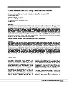
Since we have the analytic solution (2.2) we are ready to compare it with a discrete approximate solution to equation (2.3)-(2.4). The results of the comparisons are shown in Figures 2.2-2.4 and explained in Chapter 2.2.2. The solution to the equation (2.3)-(2.4) is shown in Figure 2.1.

2.1.1

A First Simple Application

Let c(t) > 0 for t > 0 be a differentiable function with the conditions c′ (t) 6= 0 and c(0) = 0. Then the solution π X(t, x) = e−c(t) sin( x) 2

(2.5)

is the unique solution to the partial differential equation Xt (t, x) −

π2 Xxx (t, x) = 0 4c′ (t)

(2.6)

ˆ x) in Table 2.1 with the conditions (2.4). Assume we are given the data X(t, 1 2 for the times t = 3 and t = 3 and want to estimate k1 = c′ ( 31 ) and k2 = c′ ( 23 ) in equation (2.6) with conditions (2.4). The idea is that c(t) is linearized to k1 t for t = 13 and c(t) is linearized to k2 t for t = 32 . To estimate k¯p for p = 1, 2 in each known point (t, x) one may use following formula

ˆ p , x) X( 1 3 k¯p = − ln t sin( π2 x) 23

(2.7)

CHAPTER 2. CREATING SYNTHETIC DATA 2

Solution with constant conductivity σ=4/π

1

Heat X

0.8 0.6 0.4 0.2 0 2 1.5

1 0.8

1

0.6 0.4

0.5 Space x

0.2 0

0

Time t

Figure 2.1: The unique solution (2.2) to the heat equation (2.3) with initial and boundary conditions (2.4).

derived from equation (2.5) with c(t) = kt and then use the values in Table 2.1. The estimates k¯1 and k¯2 from data in Table 2.1 are given in Table 2.2. As can be seen in Table 2.2 the sample variance for all estimated linearized k¯ seems to decay over time which in turn might rise some suspicion that noise is involved in the data and that this noise cancels itself over time. Instead of taking means for k¯1 and k¯2 as a final estimate, one can instead use regression. By finding a k¯1 that minimizes the summed square of errors 19 X

¯ 1 , n∆x) − X( ˆ 1 , n∆x))2 = 0.0045 (X( 3 3 n=1 we obtain k¯1 = 0.9037 and by finding a k¯2 that minimizes the summed square of errors 19 X ¯ 2 , n∆x) − X( ˆ 2 , n∆x))2 = 0.0011 (X( 3 3 n=1 we obtain k¯2 = 0.8975. Notice that the optimal constants k¯1 and k¯2 are slightly off their means of k¯1 and k¯2 respectively. To obtain c¯(t) one could second order ¯ ¯ polynomial fit c¯(t) such that c¯(0) = 0, c¯( 31 ) = k31 and c¯( 23 ) = 2k32 . 24

2.2. CHOOSING DISCRETE SYNTHETIC DATA TO THE MODEL PROBLEM

space x 0.1 0.2 0.3 0.4 0.5 0.6 0.7 0.8 0.9 1.0 1.1 1.2 1.3 1.4 1.5 1.6 1.7 1.8 1.9

ˆ 1 , x) heat X( 3 0.1157 0.2361 0.3538 0.4600 0.5486 0.6183 0.6709 0.7086 0.7322 0.7406 0.7307 0.6996 0.6473 0.5778 0.4970 0.4098 0.3176 0.2197 0.1143

ˆ 2 , x) heat X( 3 0.0863 0.1661 0.2397 0.3087 0.3736 0.4331 0.4837 0.5209 0.5420 0.5474 0.5394 0.5204 0.4913 0.4516 0.3997 0.3344 0.2567 0.1710 0.0838

Table 2.1: Some given data to the model problem. The data is given at the times t = 13 and t = 32 .

2.2

Choosing Discrete Synthetic Data to the Model Problem

One can create discrete data by quite many different means. The methods I tested are finite difference method and finite element method in space. For stepping in time I chose the forward Euler method, modified midpoint method and backward Euler method. The stencil when using finite difference method is of 3 points and the interpolating functions in the finite elements method ¯ for X and piecewise constant approxiare piecewise linear approximations X mations σ ¯ for σ.

2.2.1

Discrete Representations of the Model Problem

The next task is to derive the weak formulation to equation (1.1). There are standard examples similar to our heat equation with weak formulation in section 1.1.1 in [4], section 6.2.2 in [7], section 5.3 in [6] and section 1.5 in [8]. 25


space x 0.1 0.2 0.3 0.4 0.5 0.6 0.7 0.8 0.9 1.0 1.1 1.2 1.3 1.4 1.5 1.6 1.7 1.8 1.9 mean k¯ variance k¯

estimated k¯1 0.9043 0.8068 0.7478 0.7353 0.7615 0.8067 0.8514 0.8830 0.8979 0.9011 0.9043 0.9212 0.9586 1.0099 1.0575 1.0824 1.0720 1.0232 0.9406 0.9087 0.0116

estimated k¯2 0.8924 0.9317 0.9579 0.9658 0.9568 0.9371 0.9164 0.9030 0.9001 0.9039 0.9073 0.9043 0.8928 0.8745 0.8556 0.8460 0.8554 0.8878 0.9356 0.9066 0.0012

Table 2.2: The constant k¯p is estimated by formula (2.7) by use of the data given in Table 2.1. Notice how the sample variance is much smaller for the sample mean E[k¯1 ] = 0.9066 at time t = 13 than for the sample mean E[k¯2 ] = 0.9087 at time t = 23 .

Multiply equation (1.1) by some admissible test function φ = φ(x) such that φ(0) = φ(2) = 0 and then partial integrate with respect to x from 0 to 2 to obtain the weak formulation to (1.1) such that Z

0

2

[Xt (t, x) − (σ(t, x)Xx (t, x))x ]φ(x) dx = =

Z

0

2

Xt (t, x)φ(x) + σ(t, x)Xx (t, x)φ′ (x) dx− − [σ(t, x)Xx (t, x)φ(x)]20 = =

Z

0

2

Xt (t, x)φ(x) + σ(t, x)Xx (t, x)φ′ (x) dx = 0 (2.8) 26


which we write in bilinear form as (Xt , φ) = −(σXx , φ′ ).

(2.9)

The idea with the weak formulation is that if there is a large class of functions, preferably an infinite amount of admissible test functions φ, such where the weak formulation holds, then with appropriate regularization assumptions on σ, the integrand inside the weak formulation can be assumed pointwise zero. The next purpose is to write the bilinear form (2.9) as a linear system by some smart choice of test functions φ. Let h = N2 for some N ∈ N and define the basis functions   

φk (x) =  

1 (x h 1 − h (x

− kh) + 1, x ∈ [(k − 1)h, kh] ∩ [0, 2] − kh) + 1, x ∈ [kh, (k + 1)h] ∩ [0, 2] 0, x ∈ / [(k − 1)h, (k + 1)h] ∩ [0, 2]

(2.10)

for k = 0, . . . , N and Galerkin approximate X by the interpolating function ¯ such that X N X ¯ X(t, k∆x)φk (x). X(t, x) ≈ X(t, x) = k=0

When using Galerkin approximations in the weak formulation it is called the Galerkin method or finite elements method. My favorite text that explains the Galerkin method is [4]. The texts [6],[7],[8] also explain the Galerkin’s method. By reference to the texts [4],[6],[7] and [8], I leave it to any reader in doubt to further examine convergence for any approximation used in this thesis. Make piecewise constant approximations of the conductivity by use of the approximate points σ ¯nm such that σ ¯nm =

m σn+1 + σnm 2

(2.11)

and then approximate σ by σ ¯ (t, x) such that it becomes piecewise constant, that is σ(t, x) ≈ σ ¯ (t, x) =

−1 M −1 N X X

σ ¯nm I[(m− 1 )∆t,(m+ 1 )∆t) (t)I[n∆x,(n+1)∆x) (x) 2

m=0 n=0

2

where we have N steps in space and M steps in time. By this approximation, notice that the convention of the notation I have made in section 1.2 still holds, since σ ¯nm = σ ¯ (m∆t, n∆x). That I have chosen an average in (2.11) is 27


not necessary. As some sloppy explanation, the choice of average as in (2.11), m is an approximation to intermediate step “σn+ 1 ” which is found in following 2 finite difference approximation

Dx (σnm Dx Xnm )

≈

Dx (σnm

m m Xn+ 1 − X n− 1

)≈ ∆x m m m m m Xn − Xn−1 m Xn+1 − Xn − σn− 1 ≈ ≈ σn+ 1 2 2 (∆x)2 (∆x)2 m m m − Xnm σnm + σn−1 Xnm − Xn−1 σ m + σnm Xn+1 − = ≈ n+1 2 (∆x)2 2 (∆x)2 m m Xm − Xm m Xn − Xn−1 =σ ¯nm n+1 2 n − σ ¯n−1 . (2.12) (∆x) (∆x)2 2

2

By using the differencing operator ∆− as a backward difference operator such m that ∆− Xnm = Xnm − Xn−1 and by using ∆+ as a forward difference operator m m such that ∆+ Xn = Xn+1 − Xnm we get from (2.12) that m m m Xn+1 − Xnm m Xn − Xn−1 − σ ¯ = n−1 (∆x)2 (∆x)2 m Xm − Xm ∆+ Xnm m ∆+ Xn−1 ¯nm = ∆ σ ¯ (2.13) = ∆− σ ¯nm n+1 2 n = ∆− σ + n−1 (∆x) (∆x)2 (∆x)2

¯nm Dx (σnm Dx Xnm ) ≈ σ

which one can easily verify has the same result if one uses the central difference operator only. To derive a stiffness matrix and a load vector we fix time at ¯ t = m∆t and use the approximations X(m∆t, x) and σ ¯ (m∆t, x) in the bilinear form (2.9) to obtain

¯ x (m∆t, x), φ′ (x)) = (¯ σ (m∆t, x)X k Z k∆x Z (k+1)∆x ¯ ′ ′ ¯ X (m∆t, x) X (m∆t, x) m m =σ ¯k−1 dx − σ ¯k dx = ∆x ∆x (k−1)∆x k∆x m ¯m ¯m − X ¯m ¯m X k m ∆+ Xk−1 m Xk − Xk−1 −σ ¯km k+1 = ∆+ σ ¯k−1 (2.14) =σ ¯k−1 ∆x ∆x (∆x)2 28


and 1 Z k∆x ¯ t (m∆t, x)(x − (k − 1)∆x) dx+ ¯ X (Xt (m∆t, x), φk (x)) = ∆x (k−1)∆x 1 Z (k+1)∆x ¯ Xt (m∆t, x)(−x + (k + 1)∆x) dx = + ∆x k∆x Z 0 1 ¯ t (m∆t, x + k∆x)(x + ∆x) dx+ = X ∆x −∆x 1 Z ∆x ¯ + Xt (m∆t, x + k∆x)(−x + ∆x) dx = ∆x 0 m ¯m − X ¯ k−1 1 Z0 X ¯ km ]t (x + ∆x) dx+ x+X = [ k ∆x −∆x ∆x ¯m − X ¯m 1 Z ∆x X k ¯ km ]t (−x + ∆x) dx = x+X [ k+1 + ∆x 0 ∆x m m hX ¯ km − X ¯ k−1 ¯m − X ¯ k−1 ¯m X X ¯ km ∆x− ∆x − k ∆x − k ∆x + X = 3 2 2 i ¯m − X ¯ km ¯m − X ¯ km ¯m X X X ¯ km ∆x = − k+1 ∆x − k ∆x + k+1 ∆x + X t 3 2 2 h ∆x i ¯ m + 2∆x X ¯ m + ∆x X ¯m = (2.15) X k 6 k+1 3 6 k−1 t for k = 1, . . . , N − 1. The operator D+ is already defined in Chapter 1.2 but as a reminder I define it again as ¯ ↓m − X ¯ ↑m X m ¯ D+ Xl = ∆x which is quite convenient, since Matlab seems to compute faster by use of the diff command than by corresponding matrix multiplication. Using the results (2.14) and (2.15) in the bilinear equation (2.9) we have that m m i ¯ k−1 ∆+ σ ¯k−1 ∆+ X ¯m + 2X ¯m + 1X ¯m = X 6 k+1 3 k 6 k−1 t (∆x)2

h1

for k = 1, . . . , N − 1 which forms the systems of linear equations ¯ tm = D+ (¯ ¯ lm ) BX σ↑m · D+ X 29


where the (N − 1) × (N − 1)-matrix B is either the identity matrix, which is used for the finite difference method, or 

B=

4   1 

1  6  



1   4 1   ... ... ...   1 4 1   1 4

which is used for the finite element method. Notice that σ ¯↑m

σ↓m + σ↑m = 2

which is corresponds to the average (2.11). Discretizing in time and using the trice parameter β then we have that m+β ¯ ¯ m+β ¯ m+1 − X ¯ m ) = hD ¯ h¯ B(X iD+ Xl . + σ↑

¯ is a (N − 1) × N -matrix and D ¯ + is a N × (N + 1)-matrix. Notice that D + For a more compact notation, define the (N − 1) × (N − 1)-matrix A¯m+β such that m+β ¯ ¯ m ¯ h¯ ¯m = D A¯m+β X iD+ Xl + σ↑ in where we took use of the boundary condition X(t, 0) = X(t, 2) = 0. By use of above results we write equation (1.1) in discrete form as ¯ m+1 − X ¯ m ) = hA¯m+β X ¯ m+β B(X

(2.16)

which after some rearrangement gives ¯ m+1 = [B + h(1 − β)A¯m+β ]X ¯m [B − hβ A¯m+β ]X

(2.17)

for m = 0, . . . , M − 1. There is a finite element method for the heat equation described in Chapter 16 in [7] with discussion of stability and error estimates. The heat equation is a parabolic equation and Chapter 8 in [8] is about discretization and errors of solutions to parabolic equations as well as the text [6] has several Chapters considering error analysis for parabolic equations. Error analysis in this text is in Chapter 2.4. To study the error in recovered conductivity can be quite interesting, since recovered parameters can be used in other equations. However, I will not put any emphasis on parameter recovery in this thesis. What I do, is from a 30


handful amount of given data points recover the remaining data points. Then from these recovered data points it is possible to compute a parameter surface. Assuming X(t, x) solves the heat equation (1.1), and if I had an approximate ¯ x) for every grid point, then I would choose to estimate the solution X(t, ¯ βtr ,...,M −1+βtr from parameter space σ ¯ xX ¯ β,...,M −1+β = σ ¯ β,...,M −1+β · D

1 ¯ −1 ¯ 1,...,M ¯ 0,...,M −1 ] D [X −X ∆t x

(2.18)

¯ 0,...,M from σ and then interpolate and extrapolate σ ¯ β,...,M −1+β . There are additional ways to recover the conductivity, which I personally think are not as good as (2.18). One additional way is discussed in Chapter 3.4.6 and in ¯ 0,...,M by use of equathe Chapters 4.1.2-4.1.3. The method by obtaining σ 0,...,M ¯ tion (2.18) requires that X is known and the reason why the method by 0,...,M ¯ by use of equation (2.18) is preferred is that it is directly obtaining σ linked to its corresponding PDE while other methods do not have as close relationship to the corresponding PDE. Since data from the real world does not normally use forward Euler method or backward Euler method or some method in between for stepping in time, I have chosen to generate data by different stepping methods and then to recover remaining data by the same or different stepping methods. In real world applications, it may be very difficult to decide what stepping method is for best practice, so some tests with synthetic data can be valuable in choosing methods.1 As is explained in Chapter 4.2.2 sometimes one fails to obtain a good solution when there are different trice parameters for synthetic data and solved data. Sometimes there is noise added into different parts of data to examine convergence and robustness of the numerical algorithms. In Chapter 2.2.2 I study the effects from noise in the conductivity. In designing synthetic data presented in this thesis, I did not expand (σXx )x into σx Xx + σXxx even thought I myself designed σ(t, x). Using σx Xx + σXxx together with a time derivative Xt reminds about the convection-diffusion equation and for such equations there are plenty of methods and schemes one can use and discussing these methods are out of the scope of this degree project. Stability for our numerical schemes are discussed further in Chapter 2.4. 1

A possible improvement for generating data is to try more accurate Runge-Kutta methods. These types of tests are not done in this thesis.

31


2.2.2

Comparison of Different Synthetic Data and Experiments with Noisy Heat Conductivity

For testing purpose and to make it very simple for us, we choose σ = π42 in the whole domain to get that A¯m = A¯ is constant, such that equation (2.17) becomes ¯X ¯ m+1 = [B + h(1 − β)A] ¯X ¯m [B − hβ A]

that we rearrange and use together with a given discrete initial condition X(0, x) = X 0 to get ¯ m = (I − h[B − hβ A] ¯ −1 A) ¯ mX 0. X

When the matrix B = I∆x then the method is the finite difference method, which is sometimes preferred for slightly faster computations. Notice that with a small step ∆x that BX ≈ X∆x for B obtained from the finite element method. It is intuitive to assume that the error grows the further one steps, so therefore I choose to examine the error at the final step X M . For N = 20 steps in space and M = 12 steps in time my Matlab code yielded an error that was acceptable for β ≥ 0.05 with B derived from the finite elements method. It is possible to extend the domain [ 12 , 1] for β if one shortens the time step as is explained in Chapter 2.4. To reduce the step length in space when using the forward Euler method for stepping in time does not really help in reducing the error. The sum of squared errors X ¯ M n

ˆˆ M 2 (Xn − X n )

for different β by the finite difference method is plotted in Figure 2.2 with the error 2.4335·10−3 for the forward Euler method (β = 0), the error 2.4165·10−3 for the backward Euler method (β = 1) and the error that takes the minimal value 4.7185 · 10−8 at β = 0.48. Having β = 0.48 is almost the modified midpoint method. In Figure 2.3 we got results from a grid with N = 20 steps in space and M = 120 steps in time where one can see that the error at time t = 1 is the lowest for β = 0.25. In Figure 2.4 we got results from a grid with N = 200 steps in space and M = 48000 steps in time where one can see that the error is the lowest for forward Euler method when stepping in time. The conclusion I make from the experiment in comparing data generated by the finite element method and data generated by the finite difference method 32


is that they are quite similar when β ≥ 21 . To use the finite difference method is a bit faster than the finite element method. Experimentation showed that when having β ≤ 12 , the finite differences method is to prefer over the finite element method since if the finite differences method diverged also the finite elements method on the same grid diverges. On the other hand by experimentation, when the finite elements method diverges it showed there is still possibility for the finite element method to converge. If there is any doubt on what is a good method for the heat equation, then to be on the safe side, I suggest that one uses anything between and including the modified midpoint method and backward Euler method for stepping in time. −5

N=20, M=12, B is identity matrix

x 10 12

average of squared displacements

10

8

6

4

2

0

0.1

0.2

0.3

0.4

0.5 β

0.6

0.7

0.8

0.9

1

Figure 2.2: Error at the time t = 1 with respect to trice parameter β. The finite difference method was used to obtain this plot.

Until this point, the conductivity was constant. If the conductivity is allowed to change, obtaining an exact solution becomes more difficult if not impossible. To create synthetic data, it is preferable with respect to stability to use anything from the modified midpoint method to the backward Euler method when the dimension of the grid is N = 20 steps in space and M = 12 steps in time. To generalize the model for heat conductivity, we extend it by allowing the conductivity to change in both time and space. Let σ(t, x) =

σ+ + σ− σ+ − σ− + sin(2πx) sin(3πt) 2.2 2.2 33

(2.19)


−6


x 10


2.5

2

1.5

1

0.5

0

0.1

0.2

0.3

0.4

0.5 β

0.6

0.7

0.8

0.9

1


−11


x 10


6

5

4

3

2

1 0

0.1

0.2

0.3

0.4

0.5 β

0.6

0.7

0.8

0.9

1


34

2.2. CHOOSING DISCRETE SYNTHETIC DATA TO THE MODEL PROBLEM Conductivity

0.5 0.4 0.3 0.2 2 1

1.5

0.8 1

0.6 0.4

0.5 Space x

0.2 0

0

Time t

Figure 2.5: Plot of the conductivity (2.19) which is without noise and taking 4.8 3.2 values in the interval [ 1.1π 2 , 1.1π 2 ]. with σ+ and σ− such that σ+ =

4 4 + 2 2 π 5π

and

4 4 − 2. 2 π 5π Adding 10% noise to the conductivity σ(t, x) is done by σ− =

σ(t, x) = [

σ+ + σ− σ+ − σ− + sin(2πx) sin(3πt)](0.9 + 0.2W (t, x)) 2.2 2.2

(2.20)

where W (t, x) is a random variable from the uniform distribution such that W (t, x) ∈ [0, 1]. The conductivity (2.19) can be seen in Figure 2.5 and the conductivity (2.20) can be seen in Figure 2.6. The conductivity (2.19) yields ˆ clean , shown in Figure 2.7. The conductivity (2.20) the approximate solution, X ˆ noise , with noise. The relative error yields an approximate solution, X ˆ noise (n∆x, m∆t) − X ˆ clean (n∆x, m∆t) X ˆ clean (n∆x, m∆t) X is shown in Figure 2.8 and the squared error ˆ noise (n∆x, m∆t) − X ˆ clean (n∆x, m∆t)]2 [X 35

CHAPTER 2. CREATING SYNTHETIC DATA Conductivity with 10% noise

0.5 0.4 0.3 0.2 2 1

1.5

0.8 1

0.6 0.4

0.5 Space x

0.2 0

0

Time t

Figure 2.6: Plot of the conductivity (2.20). Here the noise has the amplitude 10% such that the conductivity takes values in the interval [ 3.2 , 4.8 ]. π2 π2

is shown in Figure 2.9. One can see that the relative noise in the solution with sample standard deviation 2.5185 · 10−3 is smaller than the relative noise in conductivity which has the sample standard deviation 2.1089 · 10−2 . Considering input noise (noise in conductivity) and output noise (noise in solution) the noise is reduced by an order of 10. Using the modified midpoint method we get input noise to 2.1089 · 10−2 and output noise to 2.2338 · 10−3 which again is a reduction of order 10. Plots when using the modified midpoint method for discretizing in time give very similar figures to those given in Figure 2.9 and are not shown here. Other sizes of grids as well as other finite difference discretizations also showed that most of the noise is near the boundary of x. By manipulating the noise in different ways I was never able to find out any reason why the noise is larger at the boundaries, even thought I removed the noise in σ near the boundaries. A possibility is that errors somewhat cancel each others far from the boundaries. If one was to recover parameters from a solution, then I think that estimates near the boundaries are those that are most off and most difficult to estimate accurately. Normally for inverse problems, we measure values and not parameters and therefore we should instead apply noise on synthetic data as is done in Chapter 4.2. 36

2.3. CHOOSING SYNTHETIC DATA TO THE FINANCE PROBLEM Heat without noise

1 0.8 0.6 0.4 0.2 0 2 1.5

1 0.8

1

0.6 0.4

0.5 Space x

0

0.2 0

Time t

Figure 2.7: Discrete solution when the conductivity is given by (2.19). The backward Euler method was used for stepping in time. Notice the small bumps on the surface.

2.3

Choosing Synthetic Data to the Finance Problem

Let there be N steps in strike (space) and M steps in maturity (time). Let the volatility σ for the price changes of timber be Gaussian with the fixed value σ = 0.2. Assume the price of timber right now is 1C$ and Mr. J Timbo is ready to pay right now X(1, x) · 5.9 · 104 C$ for an European call option giving him the right, but not obligation, to buy 59k units of logs for the price x · 5.9 · 104 C$ at the time of maturity t = 1 sun cycles from today. Let N (·) be the cumulative distribution function of the standard normal distribution. The price for one European call option, for one unit of timber, by the Black-Scholes formula in our case becomes

√ √ 5 t t 5 X(t, x) = N − √ ln x + − N − √ ln x − x. 10 10 t t

37

(2.21)

CHAPTER 2. CREATING SYNTHETIC DATA Relative error from noise

0.03 0.02 0.01 0 −0.01 −0.02 −0.03 2 1.5

1 0.8

1

0.6 0.4

0.5 Space x

0.2

0

0

Time t

Figure 2.8: Relative error in the solution caused by the noise in the conductivity (2.20). What we see is the solution with conductivity (2.20) divided by the solution with conductivity (2.19) less one. The backward Euler method was used for stepping in time. The price for the contract is the current price and changes by time.2 Discretizing the Dupire’s equation we get that

with

^ ¯ m+1 − X ¯ m = h σ (m + β)h, x 2 x2 · D ¯ 2X ¯ m+β X 2 

^ 2  σ (m + β)h, x x2 =  

which in our special case simplifies to

that we rearrange into

2

(¯ σ1m+β ∆x)2 .. . m+βtr 2 (¯ σN −1 (N − 1)∆x)

   

¯ 2X ¯ m+β ¯ m+1 − X ¯ m = h hxf2 iD X 50

¯ m = (I + [I − β h hxf2 iD ¯ 2 ]−1 h hxf2 iD ¯ 2 )m X 0 X 50 50

See for example [17] for the full formula.

38

2.3. CHOOSING SYNTHETIC DATA TO THE FINANCE PROBLEM Squared error from noise −5

x 10

3 2.5 2 1.5 1 0.5 0 2 1.5

1 0.8

1

0.6 0.4

0.5 0

Space x

0.2 0

Time t

Figure 2.9: Sum of squared errors in the discrete points. What is shown here is the sum of squared differences between the solutions, where the difference in the solutions is the solution with conductivity (2.20) less the the solution with conductivity (2.19). The backward Euler method was used for stepping in time.

with

 

X0 =  

max[1 − ∆x, 0] .. . max[1 − (N − 1)∆x, 0]



 . 

For the heat equation we had a smooth initial condition and we know that the error grows by time but unfortunately for the Dupire’s equation there is a troublesome discontinuity. Since there is an irregularity at X(0, 1), I have chosen to plot the whole surface for the error, such that the error Enm+β =

1 ¯ m+β ˆˆ m+β 2 (Xn −X ) n NM

is plotted for each point, m = 0, . . . , M − 1 and n = 0, . . . , N . In Figure 2.11 the result can be seen for β = 12 . The error peaks at the point (∆t, 1) which one can partially be explained by the discontinuity of the second order derivative X ′′ (0, 1). As can be seen, the error is of the size 1% compared to current price of a unit timber. The error for other trice parameters is about the same. I tried to eliminate the error by using the Black-Scholes formula at 39


the point (∆t, 1), i.e. I used the exact value at the point (∆t, 1), and noticed that the peak was reduced by about 75% and then found out that at x = 1 the remaining errors did not really get reduced nearly as much when stepping in time. One can read more about this in chapter 5.1.1. For stability analysis, one can read in chapter 2.4. Solution by BS−formula with r=0 and σ=0.2

1

Price X (C$)

0.8 0.6 0.4 1 0.2

0.8 0.6

0 2

0.4

1.5 0.2

1 0.5 0

Strike x (C$)

0

Maturity t (years)

Figure 2.10: Solution by use of Black-Scholes formula with interest rate r = 0 and with constant volatility σ = 0.2. The underlying stock has the value 1C$.

Since the Black-Scholes formula deals with a global volatility and the Dupire’s equation deals with a local volatility one should keep in mind that these volatilities are different. I used the image in Figure 2.12 to generate local volatility smiles. The white color is given the value σ = 0.15 and the black color is given the value σ = 0.25 and all intermediate values are linear interpolations between these two volatilities. The average volatility is about σ ≈ 0.2 and it varies up to about 25% from its mean. Comparing the plots between synthetic data from constant volatility and synthetic data from varying volatility, both generated by the Dupire’s equation, one can see that their difference is of order 1%, which is of same order as the difference between the solution from the Dupire’s equation with constant volatility and the solution from the Black-Scholes formula with constant volatility σ = 0.2. The difference in synthetic data, the price generated by Black-Scholes formula (2.21) with constant volatility less the price generated by Dupire’s equation with constant volatil40

2.3. CHOOSING SYNTHETIC DATA TO THE FINANCE PROBLEM

BS Xhathat less flat Xhathat

−3

x 10

Price X (C$)

6 4

1 0.8

2 0.6 0 2

0.4 1.5 0.2

1

Maturity t (years)

0.5 0

Strike x (C$)

0

Figure 2.11: The difference between synthetic data generated by the BlackScholes formula with constant volatility σ = 0.2 and synthetic data generated by the same constant volatility.

Figure 2.12: The synthetic volatility smile is taken from a 242x480 pixel image. The darker color the higher volatility. Notice the constant color at the boundaries.

41


flat Xhathat less Xhathat generated from image data

−3

x 10

Price X (C$)

1 6 0.8

4 2

0.6

0 0.4

2 1.5 0.2

1

Maturity t (years)

0.5 0

Strike x (C$)

0

Figure 2.13: The difference between synthetic data generated by constant volatility σ = 0.2 and synthetic data generated by the volatility in Figure 2.12 where white color represents the volatility σ = 0.15 and black color represents the volatility σ = 0.25.

ity can be seen in Figure 2.11. The difference in synthetic data generated by different volatilities, varying or constant, using the Dupire’s equation is shown in Figure 2.13. A study of the plots in Figure 2.11 and Figure 2.13 should give an idea why it is hard to estimate the volatility parameter. For the heat equation we studied noise in conductivity. For the Dupire’s equation the result from noise is different. To show the limit in numerical computational precision to compute small numbers, allow the maturity to be t = 31 with strike x = 2 then the price with respect to volatility σ is as in Figure 2.14(a). As can be seen the price for σ = 0.15 is about e−39.2542 ≈ 8.9558·10−18 and for σ = 0.25 the price is about e−17.2939 ≈ 3.0857 · 10−8 showing that the price barely changes for σ in the interval [0.15, 0.25]. At the other boundary it is even harsher, allow the maturity to be t = 13 with strike x = 0.1 then the price with respect to volatility σ is as in Figure 2.14(b). As can be seen the price is a straight line such that the price is about e−0.1054 ≈ 0.9 for all σ ∈ [0.15, 0.25] almost as if the price is independent of σ. By using BlackScholes formula without any transform, it is quite hard to obtain accurate implied volatility when the strike is far from current underlying price S(0) 42

2.3. CHOOSING SYNTHETIC DATA TO THE FINANCE PROBLEM

and even harder when maturities are near current time t = 0. The very good news is that the price X(t, x) in Black-Scholes formula is quite insensitive to noise in volatility at the boundaries. Opposed to the case with the heat equation, which is sensitive to noise in conductivity at the boundaries, the Dupire’s equation is not sensitive to noise in volatility near the boundaries. To me, the effect from propagation of computational errors in price for strikes far from current underlying price to nearby points is unknown. For a grid with N = 20 steps in strike and M = 12 steps in maturity the infinity norm of the error is of order 10−2 as can be seen in Figure 2.11. Increasing the steps in maturity from M = 12 steps to M = 12000 steps the infinity norm of the error is still of order 10−2 as can be seen in Figure 2.15. For both grids, the synthetic data was generated by the backward Euler method by using the Dupire’s equation. Using the same method, but with N = 1000 steps in strike and M = 1000 steps in maturity, one can see that the infiniy norm for the error is reduced by a factor around 20.

Logarithm of price by BS formula with t=1/3 and x=2.

Logarithm of price by BS formula with t=1/3 and x=0.1. 1

−20

0.5

−25

0 ln(X)

ln(X)

−15

−30

−0.5

−35

−1

−40 0.15

0.16

0.17

0.18

0.19

0.2 σ

0.21

0.22

0.23

0.24

−1.5 0.15

0.25

(a) The logarithm of price X by BlackScholes formula with respect to volatility. The maturity is t = 31 and the strike is x = 2.

0.16

0.17

0.18

0.19

0.2 σ

0.21

0.22

0.23

0.24

0.25

(b) The logarithm of price X by BlackScholes formula with respect to volatility. The maturity is t = 13 and the strike is 1 x = 10 .

Figure 2.14: The logarithm of price X by Black-Scholes formula with respect 1 to volatility. The maturity is t = 13 and the strikes are x = 2 and x = 10 respectively.

43


Figure 2.15: A plot of synthetic solution by Black-Scholes formula less another synthetic solution by Dupire’s equation. There are N = 20 steps in strike and there are M = 12000 steps in maturity. The difference between the solutions is at the 10th step in strike.

2.4

Von Neumann Stability Analysis

Texts recommended for study in stability analysis are chapter 6.5 in [12] and chapter 8 in [6]. Let L be some operator and let f = f (t, x, X(t, x)) be some function. Assume we are given the equation LX(t, x) = f (t, x, X(t, x)) which ˜ ˜ we write in its discrete form as L˜X(t) = f˜(t, X(t)) with its approximation ˜ ˜ ˜ ˜ ¯ ¯ ¯ written as L¯h X(t) = fh (t, X(t)). By consistent one means ˜¯ ˜ lim L˜¯h X(t) = L˜X(t)

h→0

and that

˜¯ = f˜(t, X). ˜ lim f˜¯h (t, X)

h→0

By stability one means that L˜¯h has a uniformly bounded inverse and by convergence one means

˜¯ − f˜(t, X)| ˜¯ − L˜X(t)| ˜ ˜ = 0. lim |L˜¯h X(t) + |f˜¯h (t, X)

h→0

From Lax Equivalence theorem we know that for consistent finite difference models, the stability is necessary and also suffient condition for convergence. 44

2.4. VON NEUMANN STABILITY ANALYSIS

Figure 2.16: A plot of synthetic solution by Black-Scholes formula less another synthetic solution by Dupire’s equation. There are N = 1000 steps in strike and there are M = 1000 steps in time. The difference between the solutions is at the 500th step in strike.

Considering a heat equation with constant conductivity c, it has the partial differential equation Xt (t, x) − cXxx (t, x) = 0. (2.22) To make some stability analysis, we consider an interval for the constant c, where the interval is taken from studying the model problem, such that 2.88 5.28 ≤c≤ 2 2 π π where c is computed by assuming the heat equation in the model problem has , 5.28 ]. To consider an interval for the constant conductivity in the interval [ 2.88 π2 π2 constant c for the finance problem, it may be chosen such that 0≤c≤

1 8

3 since 0 ≤ 12 x2 σ 2 ≤ 81 for 0 ≤ x ≤ 2 and 20 ≤ σ ≤ 41 . To make stability analysis using the original equation, the Dupire’s equation, even with constant volatility is too complex. Instead we use the simplified equation (2.22) for

45


stability analysis to the Dupire’s equation. For the finane problem, when trying to recover data, a larger interval for the parameter σ is assumed, such 1 3 that 10 ≤ σ ≤ 10 yielding an interval to c such that 0≤c≤

9 . 50

Discretisize an approximation to the partial differential equation (2.22) to obtain h ¯ n+1 ¯n ¯n ¯n i ¯ n+1 ¯ n+1 ¯ n+1 − X ¯ n = hc β Xm+1 − 2Xm + Xm−1 + (1 − β) Xm+1 − 2Xm + Xm−1 X m m (∆x)2 (∆x)2 n ¯m and by assuming X = a(n)eimω as a solution one obtains the growth factor ¯ n+1 X , after some rearrangement to give Gω , defined by Gω ≡ X¯mn = a(n+1) a(n) m

Gω = 1 +

1 (∆x)2 2hc(cos ω−1)

−β

.

It is easy to see that G0 = 1 so assume for the rest of this chapter that cos ω 6= 1. Using the frequency ω = lem, we get that

π , 2

to fit the initial condition to the model prob-

G π2 = 1 −

1 (∆x)2 2hc

+β

< 1.

By von Neumann stability analysis it is considered that |Gω | ≤ 1 for all ω is a necessary and sufficient condition for stability. First consider only ω = 12 where the condition |G π2 | ≤ 1 implies (∆x)2 + 2hcβ ≥ hc which is clearly true for all trice parameters β ≥ 12 and which also seemed to be true by experimental inspection. If the trice parameter β is such that 0 ≤ β < 12 then we get that h≤

(∆x)2 (∆x)2 ≤ c(1 − 2β) c

1 and c = π42 it is a good suggestion by and by inserting the values ∆x = 10 1 von Neumann stability analysis to take the time step h ≤ 54 however as seen 1 in Figure 2.2 the synthetic data is accurate for the larger time step h = 12

46

2.4. VON NEUMANN STABILITY ANALYSIS

by the fact that we did not take enough time steps to notice any effects of divergence. Increaing the constant conductivity from σ = π42 to σ = π52 for synthetic data in the model problem on the same grid yielded synthetic data where one could start to notice slight divergence for β = 0. The results for synthetic data become interesting when allowing the conduc1 tivity vary. This time by experimental testing with step length ∆x = 10 in 1 space and step length h = 12 in time and varying conductivity (2.19) gave synthetic data that diverged as expected by the stability analysis. The synthetic data had for the time t = 1 astronomical values of order 107 . We conclude that on a grid with the dimensions N = 20 steps in space and M = 12 steps in time with varying conductivity (2.19) yield such results in synthetic data that are very different from corresponding case with constant conductivity σ = π42 . One should consider all ω to look for worst case scenarios in the von Neumann 2 stability analysis. If β = 0 then we obtain the well-known result h ≤ (∆x) 2c which is as half as much as for the case with the frequency ω = 21 . Choosing 1 the step length h = 120 should by von Neumann stability analysis be be good enough for use in the model problem for any β. 2

1 9 with ∆x = 10 and c = 50 one is For the finance problem, using h ≤ (∆x) 2c 1 suggested to take h ≤ 36 however, for the finance problem I choose to solve on a grid with the dimensions N = 20 steps in space (strike) and M = 12 steps in time (maturity). Using the knowledge that max volatility in synthetic data actually is σ = 51 it is suggested one use the slighty larger time 1 2 ≈ 12 . I used this grid for recovering data for the finance problem, step h ≤ 25 larger grids become quite computing intensive without substansial increase of accurary in the solution. They owe me more than 10 years youth of life and KTH is involved in this. Pay me for this!

47

Chapter 3 Optimal control To study optimal control theory a quick start is to look in section 10.3 in [3] that covers existence and uniqueness of Hamilton-Jacobi equations and continuous dynamic programming. In [13] one can also study optimal control theory with applications related to this degree project, especially the Pontryagin principle. Other suitable texts with optimal control related to this degree project can be found in [14],[15],[16]. ˜ Assume that in this chapter vector valued variables, such as X(t), can be ˜ extended to include one or both boundary points, for example X(t) is ex˜ tended to Xl (t), without loss of generality. The only requirement is that all vector valued variables are of such dimension that all vector and matrix operations are valid. Defining some Lagrangian and use of optimal control is explained in chapter 3.4.6. One can skip chapter 3.4.6, since what is done there is repeated in chapter 4.1. Fortunately chapter 3.4.6 is short and is more general than what is presented in chapter 4.1 since the theory in chapter 4.1 is restricted to an application using the dynamics of the heat equation only.

3.1

Definitions

Assume αmin < αmax are constants and let AN ⊂ RN where AN is such that each of its elements are in the interval A = [αmin , αmax ] ⊂ R. The set AN is ˜ = X(t) ˜ ˜ : R+ → RN denotes a N -dimensional cube. Let X be such that X ˜ the path where X(t) is the spatial discretization and vector valued function derived from its corresponding continuous path X = X(t, x) such that X : ˜ α R+ ×R → R. Let u = u(t, X, ˜ ) be a function such that u : R+ ×RN ×AN → R 49

CHAPTER 3. OPTIMAL CONTROL

which we say to be the cost function. Assume that we like to compute a cost, where we have a control α ˜=α ˜ (t) such that α ˜ : R+ → AN where α ˜ (t) is the discrete and vector valued function derived from its corresponding continuous control α = α(t, x) such that α : R+ × R → A, and where we have the running ˜ cost L[X(t), α ˜ (t)], which is a function such that L : RN × AN → R and where ˜ 1 )) such that g : RN → R we have the final cost or terminal cost g = g(X(t with t1 as final time and t0 as initial time. The times t0 and t1 are considered fixed. The total cost is expressed as the cost function u(t0 , X 0 , α ˜ ) such that ˜ 1 )) + u(t0 , X , α ˜ ) = g(X(t 0

Z

t1

t0

˜ L[X(s), α ˜ (s)] ds

(3.1)

˜ 0 ) given. The set AN is called control with the initial condition X 0 = X(t space and normally looks more complex than the one we have defined here. One may for example allow the control space depend on space and time. An example of a cost function is when Captain Red rents a phantom airship from General Ivan to transport timber from Gwens Guinea to Lake Valiente. The costs are usage of O12 fuel and the rent of the airship. Here the running cost is the use of fuel, the final cost is the rent of the phantom airship and the control is the route Captain Red drives this airship from Gwens Guinea to Lake Valiente. For more detailed examples in optimal control, see section 9.1.1. in [13], chapter 2 in [15] and chapter 3-4 in [14]. In this text, for the model problem and finance problem there are no final costs nor running costs dependent of the control, which leaves us with a cost function of the form 0

u(t0 , X , α ˜) =

Z

t1

t0

˜ L[X(s)] ds.

(3.2)

In this section, we will however use the cost function (3.1) to be somewhat more general in formulating optimal control. Assume that the control α ˜ gives us the path by following dynamics

˜˙ = f t, X(t), ˜ X α ˜ (t) ,

(3.3)

˜ for all t0 < t < t1 with given initial condition X(0) and where f is some given ˜ functional. Let ν = ν t, X(t) be a function such that ν : R+ × RN → R. Normally when attempting to compute and evaluate the following optimal cost function, ˜ ˜ ν t, X(t) = infN u t, X(t), α ˜ (s) (3.4) α∈A ˜

50

3.2. THE HAMILTON-JACOBI EQUATION

one faces several obstacles, such as existence and uniqueness among others. Real world problems are rarely well-posed as we will experience in chapter 4 and chapter 5. In this chapter we assume we have a well-posed problem. Before explaining the meaning of well-posed I explain a little about the function ν which we call for the value function. One might for some reason need to use other arguments than those that are in the value function and therefore instead define its dual with the wanted arguments, which we then call for the ˜ where v is a functional ˜ λ), dual value function denoted by the letter v = v(X, N N such that v : R × R → R. The dual function is studied further in chapter 3.4.1 and again in chapter 3.4.6. There are many different definitions on what well-posed means. One is that a unique solution exists and that the behavior of the solution hardly changes when there is a slight change in its initial condition. The definition to wellposed by Hadamard, which is used in [13], is that a unique solution exists and that the solution depends continuously on given data. A problem that is not well-posed is called ill-posed. There are several ways to minimize the cost function, such as dynamic programming, the Pontryagin minimum principle and different computational algorithms. Every approach have their advantage and disadvantage. A list about these advantages and disadvantages can be read in chapter 3.5 and they can be found in [13].

3.2

The Hamilton-Jacobi Equation

˜ be a function such that ν : R+ × RN → R and let t ∈ [t0 , t1 ] ⊂ Let ν = ν(t, X) ˜ ∈ RN . Assume H is a function such that H : [t0 , t1 ] × RN × R → R. R+ and X Hamilton-Jacobi equations are non-linear PDE of the form ˜ νx ) = 0, νt + H(t, X,

t0 < t < t1 ,

(3.5)

with initial condition ˜ 0 )) = g(X(t ˜ 0 )) ν(t0 , X(t or final condition ˜ 1 )) = g(X(t ˜ 1 )) ν(t1 , X(t where g is a known function such that g : RN → R. The function H is called the Hamiltonian. If one is given a Hamilton-Jacobi equation in the time interval [t0 , t1 ] with a terminal condition at time t1 instead of an initial condition at time t0 then by substituting t by t1 + t0 − t one gets another HamiltonJacobi equation in the same time interval [t0 , t1 ] with an initial condition at 51


t0 . With the same substitution one can substitute a Hamilton-Jacobi equation with an initial condition to get another Hamilton-Jacobi equation with a terminal condition. To study the existence of some solutions to (3.5) the approach in [3],[13] and many other texts is to consider an approximate problem to equation (3.5) such that ǫ ˜ νxǫ ) = ǫνxx νtǫ + H(t, X,

with initial condition

(3.6)

˜ = g(X) ˜ ν ǫ (0, X)

ǫ by which one hopes that the term ǫνxx regularizes the solution to (3.5). The method by letting a positive ǫ → 0 is called vanishing viscosity. In chapter 10.1 in [3] there is a motivation for using vanishing viscosity solutions as well as the consistency of viscosity solutions to equation (3.5) is showed. Reading further into chapter 10.2 in [3] one can see that Theorem 1 states there exists at most one viscosity solution to (3.5). The idea by choosing viscosity solutions is to circumvent different problems, such as jumps, infinite derivatives among many other obstacles. One says the solution is regularized when adding viscosity to counter these nasty obstacles, i.e. if possible, then by regularization one tries to approximate the problem by a well-posed viscosity solution.

3.3

Lipschitz Continuity

We need some way to measure the distance between points. For some space M , assume there is an associated distance function, a so called metric, d : M × M 7→ R such that it holds for all x, y, z ∈ M , 1. d(x, y) ≥ 0, 2. d(x, y) = 0 if and only if x = y, 3. d(x, y) = d(y, x), 4. d(x, y) ≤ d(x, z) + d(z, y), for points x, y, z ∈ M . If there exists some metric for all points in M then (M, d) is said to be a metric space. The first condition is called the nonnegativity condition, that is to ensure that we do not have a negative distance. The second condition says that we only have the distance 0 for points at the same location, or that points in same location have the distance zero. The third condition is a symmetry condition, that says that the distance from x to y is the same as the distance from y to x. Finally, the fourth condition is 52

3.3. LIPSCHITZ CONTINUITY

a triangle inequality, which says that the distance between two points x and y is less or equal to the distance between the two points via a third point z. A function f : M 7→ N , where (M, d) and (N, d) are metric spaces, is said to be Lipschitz continuous if there exists some constant K > 0 such that d(f (x), f (y)) ≤ Kd(x, y) for all x, y ∈ M . Assume f (x) is Lipschitz continuous in M and let [a, b] ∈ M then with the metric d(x, y) = |x−y| and by definition of the derivative and by the definition of Lipschitz continuity we have that |f ′ (x)| = lim | h→0

f (x + h) − f (x) d(f (x + h), f (x)) | = lim ≤ h→0 h d(0, h) Kd(x + h, x) ≤ lim = lim K = K. (3.7) h→0 h→0 d(0, h)

That f (x) is Lipschitz continuous yields itself −K|x − a| + f (a) ≤ f (x) ≤ K|x − a| + f (a).

(3.8)

With Lipschitz continuity with the same metric in integrals one obtains Z

b

a

Z f (x) − f (a) dx ≤

b

a

|f (x) − f (a)| dx ≤ K

Z

b

a

|x − a| dx = =

K (b − a)2 (3.9) 2

which yields −

Z b K K (b − a)2 + f (a)(b − a) ≤ f (x) dx ≤ (x − a)2 + f (a)(b − a). (3.10) 2 2 a

One may obtain K by K = sup |f ′ (x)|, x∈M

which is called the Lipschitz constant provided f is differentiable. When f is a function of several variables, for example x1 , . . . , xn , then we may call f Lipschitz continuous with respect to xk , if f is Lipschitz continuous when all variables except xk are held constant. A function f with its domain in a metric space (M, d), is said to be uniformly continuous, if for every real number ǫ > 0 there exists a δ > 0 such that d(f (x), f (y)) < ǫ for all d(x, y) < δ. It can be shown that all Lipschitz continuous functions are uniformly continuous and that all uniform continuous functions are continuous, but one cannot guarantee that a continuous function is Lipschitz continuous nor uniformly continuous. 53


An example of continuous function that is not Lipschitz continuous neither uniform continuous is f (x) = x1 for M = (0, 1]. So we remark here that if a function is Lipschitz continuous then we usually are more than satisfied with that than with a continuous function and if Lipschitz continuity is easy to show then one should use it.

3.4 3.4.1

The Hamilton Characteristics Method by Lagrange

Before deriving the Pontryagin principle we look at its predecessor in optimization. Assume that we have the real valued function F = F (x, y) subject to y = f (x) that we seek to optimize F (x, y) with respect to x. At optimum it follows that d F (x, f (x)) = Fx + Fy fx = 0. dx

(3.11)

An alternate method, by Lagrange, is to define G = G(x, y, λ) such that G(x, y, λ) = F (x, y) + λ[y − f (x)] then if Gx = Fx − λf ′ = 0 and Gy = Fy + λ = 0 and Gλ = y − f (x) = 0 then critical F is reached which is quite easy to validate. The variable λ is called Lagrange multiplier and the function G is called Lagrangian. Assume we want to minimize the cost ˜ 1 )) + g(X(t

Z

t1

t0

˜ L[X(s), α ˜ (s)] ds

with respect to the control α ˜ (s) and subject to the dynamics (3.3) which is ˜˙ ˜ X(t) − f (t, X(t), α ˜ (t)) = 0. 54

3.4. THE HAMILTON CHARACTERISTICS

Notice that the cost is the same as in (3.1). Multiply by the Lagrange mul˜ tiplier −λ(t) into the dynamics and integrate from t0 to t1 to form the Lagrangian ˜ α ˜ λ, L(X, ˜ ; t0 , X 0 ) = ˜ 1 )) + = g(X(t

Z

t1

t0

˜ ˜ ˜˙ ˜ L[X(s), α ˜ (s)] − λ(s)[ X(s) − f (s, X(s), α ˜ (s))] ds (3.12)

˜ 0 ) and form the dual value function where X 0 = X(t ˜ = g(X(t ˜ λ) ˜ 1 )) + v(X,

Z

t1

t0

˜ ˜ ˜˙ ˜ L[X(s), α ˜ ∗ (s)] − λ(s)[ X(s) − f (s, X(s), α ˜ ∗ (s))] ds

(3.13) where α (s) ∈ A is some optimal control. Partial differentiation with respect ˜ on the Lagrangian (3.12) as is done in chapter 3.4.6 yields the equation to λ of dynamics (3.3). It remains to motivate, which is done in chapter 3.4.6, that the Lagrangian with an optimal control α∗ which is the dual value function ˜ has the same optimal control and value as ν(t, X(t)). ˜ λ) ˜ v(X, ∗

3.4.2

N

Some Property of the Optimal Control

Let t and h > 0 be such that t0 ≤ t < t + h ≤ t1 . The optimal control α ˜∗ = α ˜ ∗ (s) ∈ AN is derived in chapter 3.4.3. In this chapter we mostly assume the optimal control α ˜ ∗ is known for the time interval s ∈ [t + h, t1 ]. Having the optimal control α ˜ ∗ for the time interval s ∈ [t, t1 ] it naturally follows by the definition (3.4) that ˜ ν(t, X(t)) =

Z

t

t+h

˜ ˜ + h), α L[X(s), α ˜ ∗ (s)] ds + u(t + h, X(t ˜ ∗ |[t+h,t1 ] )

where α ˜ ∗ |[t+h,t1 ] = α ˜ ∗ |[t+h,t1 ] (s) is the control α ˜ ∗ in the interval [t + h, t1 ]. Suppose the control α ˜ ∗ |[t+h,t1 ] is not optimal over [t + h, t1 ] then there exists ∗∗ another control α ˜ |[t+h,t1 ] = α ˜ ∗∗ |[t+h,t1 ] (s) ∈ AN for the times s ∈ [t + h, t1 ] such that ˜ ν(t, X(t)) >

Z

t

t+h

˜ ˜ + h), α L[X(s), α ˜ ∗ (s)] ds + u(t + h, X(t ˜ ∗∗ |[t+h,t1 ] )

(3.14)

but by definition, for any control α ˜=α ˜ (s) ∈ AN , we have that ˜ ˜ ˜ ν(t, X(t)) = u(t, X(t), α ˜ ∗ ) ≤ u(t, X(t), α ˜ ).

(3.15)

The inequality (3.14) is a contradiction to the inequality (3.15) yielding that the control α ˜ ∗∗ does not exists and therefore we conclude that α ˜ ∗ which is an 55


optimal control in the time interval [t, t1 ] is also an optimal control in the time interval [t + h, t1 ]. Assuming we have the optimal control α ˜ ∗ (s) for the time interval [t + h, t1 ]. Then by above result by h → 0 we have that the control α ˜ ∗ (s) is also optimal for the time interval (t, t1 ]. Knowing that α ˜ ∗ (s) is the optimal control in the time interval [t, t1 ] assume there exists some control α ˜ ∗∗ |[t,t+h) = α ˜ ∗∗ |[t,t+h) (s) such that Z

t

t+h

˜ L[X(s), α ˜ ∗ (s)] ds >

Z

t+h

t

˜ L[X(s), α ˜ ∗∗ |[t,t+h) (s)] ds

˜ then the value function ν(t, X(t)) is not optimal and contradicting its own definition (3.15) yielding that the control α ˜ ∗∗ |[t,t+h) does not exists and therefore Z t+h Z t+h ∗ ˜ ˜ L[X(s), α ˜ (s)] ds ≤ L[X(s), α ˜ (s)] ds t

t

for any control α ˜ (s). Assuming we have the optimal control α ˜ ∗∗ |[t,t+h) (s) for the time interval [t, t + h). Then by above result by h → 0 we have that the control α ˜ ∗ (s) is also optimal for the point s = t. To obtain an optimal control for the interval [t, t1 ] it is enough to find the optimal control to every point s ∈ [t, t1 ].

3.4.3

Obtaining the Hamilton-Jacobi-Bellman Equation by Continuous Time Dynamic Programming

Dynamic programming is explained in many courses in optimization. For a thorough explanation with examples on discrete dynamic programming a text to look into is [5]. Dynamic programming for the continuous case are explained in [3],[13]. Assume we want to minimize (3.1) with given dynamics (3.3). The idea with dynamic programming is to track its solution backwards in time, that is we ˜ + h)) and then look for ν(t, X(t)). ˜ already have ν(t + h, X(t The derived equation, which is a result from trying to find the solution backwards when taking the limit h → 0 is called the Hamilton-Jacobi-Bellman equation and its proof can be found in Theorem 2 in section 10.3.3 in [3]. Here below comes a quick and dirty derivation of the Hamilton-Jacobi-Bellman equation. Let t and h > 0 be such that t0 ≤ t < t + h ≤ t1 . Denote the optimal control as 56


α ˜ ∗ . Consider we already have the optimal control in the interval s ∈ [t + h, t1 ] then ˜ ν(t, X(t)) =

inf N [

α(s)∈A ˜

=

Z

t+h

t

inf

N α(s)∈A ˜

˜ ˜ + h))] = L(X(s), α ˜ (s)) ds + ν(t + h, X(t

Z

t+h

t

˜ ˜ + h)). (3.16) L(X(s), α ˜ (s)) ds + ν(t + h, X(t

˜ is Lipschitz continuous and L is continuous then by taking the limit If X h → 0 we obtain ˜ α ˜ α νt + νxT f (t, X, ˜ ∗ ) + L(X, ˜∗) = 0 (3.17) subject to the final condition ˜ 1 )) = g(X(t ˜ 1 )). ν(t1 , X(t Notice that equation (3.17) is a Hamilton-Jacobi equation by equation (3.5) since ˜ νx ) = νxT f (t, X, ˜ α ˜ α H(t, X, ˜ ∗ ) + L(X, ˜∗) and further equation (3.17) is called the Hamilton-Jacobi-Bellman equation. Notice that the Hamilton-Jacobi-Bellman equation has a terminal condition and that this terminal condition is the final cost to its corresponding minimization problem (3.1). Normally, we do not have the optimal control given for the time interval [t, t1 ]. Assume that we have the optimal control for the time interval [t + h, t1 ] then we have that ˜ ν(t, X(t)) ≤

Z

t

t+h

˜ ˜ + h)) L[X(s), α ˜ (s)] ds + ν(t + h, X(t

(3.18)

where there is equality if the control in optimal and inequality if the control is ˜ not optimal. If the running cost L[X(s), α ˜ (s)] = 0 for all controls α ˜ (s) ∈ aN in the time interval [t, t + h) it follows that ˜ + h)) = ν(t, X(t)) ˜ ν(t + h, X(t

(3.19)

since there is no running cost in the time interval [t, t + h). Assume we are instead given equation (3.19) then 0=

Z

t

t+h

˜ L[X(s), α ˜ ∗ (s)] ds ≤ 57

Z

t

t+h

˜ L[X(s), α ˜ (s)] ds


˜ ∗ (s) as the optimal path where α(s) is some arbitrary control. Denote X corresponding to the optimal control α ˜ ∗ (t) and allow h → 0 then ˜ ∗ (t), α ˜ 0 = L[X ˜ ∗ (t)] ≤ L[X(t), α ˜ (t)]. What we showed is that where the running cost is zero for every admissible control then the value function does not change. We also showed that if the value function does not change then on an optimal path with corresponding optimal control the running cost is zero and with another control than an optimal control or another path than the optimal path the running cost is positive. ˜ Assume the running cost L[X(s), α ˜ (s)] is not zero in the time interval [t, t+h). Recall the inequality (3.18) 0≤

Z

t+h

t

˜ L[X(s), α ˜ (s)] ds + +

Z

t

t+h

Z

t

t+h

˜ dν(s, X(s)) =

Z

t

t+h

˜ L[X(s), α ˜ (s)] ds+

˜ ˜ ˜ νt (s, X(s)) + νX (s, X(s))f (s, X(s), α ˜ (s)) ds (3.20)

and allow h → 0 then we obtain the inequality ≤

0

˜ ˜ ˜ ˜ L[X(t), α ˜ (t)] + νt (t, X(t)) + νX (t, X(t))f (t, X(t), α ˜ (t)). (3.21)

If we have an optimal control α∗ (s) in the inequality (3.18) then the HamiltonJacobi-Bellman equation (3.17) follows. The Hamilton-Jacobi-Bellman equation (3.17) together with the inequality (3.21) gives ˜ ˜ ˜ L[X(t), α ˜ ∗ (t)] + νX (t, X(t))f (t, X(t), α ˜ ∗ (t)) ≤ ˜ ˜ ˜ ≤ L[X(t), α ˜ (t)] + νX (t, X(t))f (t, X(t), α ˜ (t)) (3.22) that we write as the following very important result

T ˜ ˜ ˜ (t) + L X(t), α ˜ (t) ]. α ˜ ∗ (t) ∈ argminα(t) ˜ [νx f t, X, α

(3.23)

The property (3.23) is called the Pontryagin principle. To be one the safe side, let us see what the inequality (3.22) really means. Integrate the inequality (3.22) from t to t + h to obtain Z

t

t+h

˜ ˜ ˜ L[X(s), α ˜ ∗ (s)] + νX (s, X(s))f (s, X(s), α ˜ ∗ (s)) ds ≤ ≤

Z

t

t+h

˜ ˜ ˜ L[X(s), α ˜ (s)] + νX (s, X(s))f (s, X(s), α ˜ (s)) ds. (3.24) 58


Use the Hamilton-Jacobi-Bellman equation (3.17) in the inequality (3.24) to obtain 0≤

Z

t

t+h

˜ ˜ ˜ ˜ L[X(s), α ˜ (s)] + νt (s, X(s)) + νX (s, X(s))f (s, X(s), α ˜ (s)) ds = = =

Z

t

Z

t+h

t t+h

˜ L[X(s), α ˜ (s)] ds +

Z

t

t+h

˜ dν(s, X(s)) ds =

˜ ˜ + h)) − ν(t, X(t)) ˜ L[X(s), α ˜ (s)] ds + ν(t + h, X(t (3.25)

which is the inequality (3.20). With the results from chapter 3.4.2 and the instantaneous optimal control (3.23) we can get the optimal control for the time interval [t, t1 ].

3.4.4

Deriving the Characteristic Equations to the Hamilton-Jacobi Equation

The Hamilton-Jacobi-Bellman equation is a special case of a Hamilton-Jacobi equation. In this chapter we deal with the characteristic equations to the Hamilton-Jacobi equation. Assume we have the Hamilton-Jacobi equation ˜ νx ) = 0 νt + H(t, X, ˜ as a vector with components λ ˜ k = ν ˜ and assume X ˜ follows and then define λ Xk the characteristic equation ˜ ˜˙ ˜ X(s) = Hλ˜ (t, X(s), λ(s)) that is

(3.26)

˜ ˜˙ k (s) = H˜ (t, X(s), ˜ X λ(s)) λk

˜ are for k = 1, . . . , d. The boundary and initial or terminal conditions for X normally given and preserved for the characteristic equation (3.26). Derive νt ˜ k to obtain with respect to X −

X ˙ ∂ ˜ + ˜ k′ ν ˜ ˜ ˜ λ) X νX˜k = HX˜k (t, X, Xk ′ Xk ∂t ′ k

which gives us the second characteristic equation ˜˙ = H ˜ (t, X, ˜ ˜ λ). −λ X

(3.27)

˜ 1 )) = g(X(t ˜ 1 )) Assuming the value function has the final condition ν(t1 , X(t ˜ ˜ ˜ it is evident that λ has the final condition λ(t1 ) = DX˜ g(X(t1 )). So if we were 59


to use the Hamiltonian from the Hamilton-Jacobi-Bellman equation (3.17) in equation (3.26) we get the dynamics (3.3) and the Hamilton-Jacobi-Bellman equation (3.17) in (3.27) gives us ˜˙ = λ ˜ T f ˜ (t, X, ˜ α ˜ α −λ ˜ ∗ ) + LX˜ (X, ˜ ∗ ). X Basically, what we have motivated in chapter 3.4.3 is that the optimal solution to (3.1) with the dynamics (3.3) also solves the Hamilton-Jacobi-Bellman equation (3.17) and in this chapter we motivated that the solution to a Hamilton-Jacobi equation (3.17) yields the Hamilton characteristic equations (3.26)-(3.27). To show the reverse, that a system of characteristic equations (3.26)-(3.27) have an existing value function subject to a certain dynamics is not always possible. The Hamilton characteristic equations (3.26)(3.27) together with the Pontryagin principle (3.23) and the final condition ˜ 1 )) = g(X(t ˜ 1 )) are necessary but not sufficient conditions for an optiν(t1 , X(t mal control. As explained in the abstract and in the introduction, the purpose in this degree project, is to obtain some characteristic equations by different means and to test if they solve their intended control problem.

3.4.5

Deriving the Value Function from the Hamilton-Jacobi-Bellman Equation

We saw in chapter 3.4.3 how continuous dynamic programming on the value function (3.16) lead to the Hamilton-Jacobi-Bellman equation (3.17). One may ask oneself what is the meaning of equation (3.17)? Now assume we go the reverse way, i.e. assume we have the Hamilton-Jacobi-Bellman equation (3.17) given. Note that we are not yet aware that α ˜ ∗ is the optimal control d in equation (3.17). By the chain rule for dt ν and by using the dynamics (3.3) we get the equation d ˜ = L(t, X, ˜ α ˜∗) − ν(t, X) dt that we integrate from t to t + h to have ˜ ν(t, X(t)) = ≥

Z

t+h

t

inf N [

α(s)∈A ˜

Z

t

˜ α ˜ + h)) ≥ L(s, X, ˜ ∗ ) ds + ν(t + h, X(t

t+h

˜ α ˜ + h))] = ν(t, X(t)) ˜ L(s, X, ˜ ) ds + ν(t + h, X(t (3.28)

˜ where the last equality holds by the definition of ν(t, X(t)). Since by definition ˜ ˜ ˜ 1 )) + ν(t, X(t)) ≤ u(t, X(t), α ˜ ) = g(X(t 60

Z

t

t1

˜ L(s, X(s), α ˜ ) ds

(3.29)


for all controls α ˜ we have that ˜ ν(t, X(t)) =

˜ 1 )) + inf N [g(t1 , X(t

α(s)∈A ˜

Z

t

t1

˜ L(s, X(s), α ˜ ) ds].

˜ We conclude that if ν(t, X(t)) solves the Hamilton-Jacobi-Bellman equation ˜ (3.17) and that X(t) has the dynamics (3.3) then its solution corresponds to the optimal value to control problem (3.1).

3.4.6

The Pontryagin Principle with an Application

In the final cost, consider now g = 0. Define the function ˜ α ˜ T f (t, X, ˜ λ, ˜ α ˜ α B(t, X, ˜ ) = L(X, ˜) + λ ˜)

(3.30)

˜ is a Lagrange multiplier and then assume we are given the Lagrangian where λ ˜ α ˜ λ, L(X, ˜ ; t0 , X 0 ) =

Z

t1

t0

˜ α ˜T X ˜ λ, ˜˙ dt B(t, X, ˜) − λ

(3.31)

˜ 0 ). For a shorter notation suppress the parameters t0 and where X 0 = X(t 0 X in L. Notice that equation (3.31) is the same as equation (3.12) but with g = 0. We said in chapter 3.4.1 that differentiation with respect to λ yielded ˜ by λ ˜ + ǫw˜ the constraint to the objective function. Therefore, substitute λ ˜ is already critical and let w˜ be some arbitrary perturbation. and assume λ Differentiate with respect to ǫ to obtain Z t1 d ˜ + ǫw, ˜ + ǫw, ˜ λ ˜˙ dt ˜ λ Bλ˜ (t, X, ˜ α ˜ )w ˜ − w˜ T X L(X, ˜ α ˜) = dǫ t0

˜ is already critical then in weak sense the equaand since w˜ is arbitrary and λ tion d ˜ + ǫw, ˜ λ lim L(X, ˜ α ˜) = 0 ǫ→0 dǫ yields the characteristic equation ˜ α ˜˙ = B˜ (t, X, ˜ λ, ˜ α X ˜ ) = f (t, X, ˜) λ

(3.32)

˜ The Lagrangian (3.31) reminds which describes as said the dynamics for X. about the cost function (3.1) and equation (3.32) reminds about the characteristic equation (3.26). Something of interest to figure out is if defining ˜ α ˜ k = ∂˜ L(X, ˜ λ, ˜ ) yields something that reminds about equation (3.27). Asλ ∂ Xk ˜ with λ ˜ k = ∂˜ L(X, ˜ α ˜ λ) ˜ λ, sume v(X, ˜ ) solves a Hamilton-Jacobi equation and ∂ Xk has such connection to our Lagrangian that there exists a control α ˜ ∗ such that 61


˜ = L(X, ˜ α ˜ λ) ˜ λ, v(X, ˜ ∗ ). If one considers the Lagrangian (3.31) as a cost func˜ becomes zero at such points where the Lagrangian tion then the function λ cannot change, and such points are at the terminal condition for the Hamilton˜ is Jacobi-Bellman equation. That the value function cannot change where X known was shown in chapter 3.4.2. ˜ = 0 as final condition since ˜ Assuming λ Next is to find the optimal path X. g = 0 then by partial integration of the cost function (3.31) we have that ˜ α ˜ λ, L(X, ˜) =

Z

t1

t0

˜ α ˜˙ T X ˜ 0 )T X(t ˜ λ, ˜ dt + λ(t ˜ 0) B(t, X, ˜) + λ

(3.33)

˜ by X ˜ + ǫw˜ with w(t in which we substitute X ˜ 0 ) = 0 since X 0 is known and then differentiate with respect to ǫ to obtain Z t1 d ˜ α ˜˙ T w˜ dt. ˜ α ˜ + ǫw, ˜ + ǫw, BX˜ (X ˜ λ, ˜ )w˜ + λ L(X ˜ λ, ˜) = dǫ t0

˜ is critical and let w˜ be some arbitrary perturbation, then Assume X lim ǫ→0

d ˜ α ˜ + ǫw, L(X ˜ λ, ˜) = 0 dǫ

and since w˜ is arbitrary it follows that in weak sense ˜˙ = B ˜ (t, X, ˜ α ˜ λ, −λ ˜) X

(3.34)

which is the second characteristic equation and indeed reminds about equation (3.27). By choosing the optimal control ˜ T f (t, X, ˜ ˜ )+λ ˜ α ˜ ˜ ˜ )] = argminα∈A ˜ )] (3.35) α ˜ ∗ ∈ argminα∈A N [L(X, α N [B(t, X, λ, α ˜ ˜ which one should compare with (3.23), we have that ˜ α ˜ ˜ λ, ˜ λ). B(t, X, ˜ ∗ ) = H(t, X, The property (3.35) is the Pontryagin principle as mentioned before in (3.23). The equations (3.32) and (3.34) are called Hamilton characteristic equations ˜ = 0 with given equations λ ˜ = v˜ ˜ λ) which one also derives from vt + H(t, X, X ˜ ˜˙ ˜ and X(s) = Hλ˜ (t, X(s), λ(s)). And if the Hamilton-Jacobi equation is a Hamilton-Jacobi-Bellman equation, then its solution is the optimal value to corresponding control problem.

62


Let us have an application using the Pontryagin principle. Assume we like to minimize Z 1 ˜ L[X(s)] ds 0

subject to the dynamics

˜˙ ˜ ′′ (t) X(t) =σ ˜ (t) · X

(3.36)

˜ ˜ with given initial condition X(0) = X 0 and final condition X(1) = 0. Define the function ˜ α ˜ T h˜ ˜ λ, ˜ +λ ˜ ′′ (t) B(X, ˜ ) = L[X] α(t)iX where h˜ α(t)i is a diagonal matrix which notation is explained in Chapter 1.2.6. Define the Lagrangian ˜ α ˜ λ, L(X, ˜) =

Z

1

0

˜ α ˜T X ˜ λ, ˜˙ dt = B(X, ˜) − λ =

Z

0

1

˜˙ T X ˜ T (0)X(0). ˜ α ˜ dt − λ ˜ ˜ λ, (3.37) B(X, ˜) + λ

Assume that the function s[·, ·] ∈ R is such that ˜ ˜ α ˜ ˜ ˜ )] = L[X(t)] ˜ ˜ ˜ λ, + s[λ(t), X(t)] B(X, ˜ ∗ ) = argminα∈A N [B(X, λ, α ˜ then ˜ α ˜ λ, L(X, ˜) =

Z

0

1

˜ ˜T X ˜ ˜ ˜˙ dt = L[X(t)] + s[λ(t), X(t)] −λ Z

0

1

˜˙ T X ˜ T (0)X(0). ˜ ˜ dt − λ ˜ ˜ ˜ (3.38) L[X(t)] + s[λ(t), X(t)] +λ

˜ to find a critical λ ˜ Differentiating the Lagrangian (3.37) with respect to λ ˜ to yields equation (3.36) and differentiating equation (3.38) with respect to λ ˜ yields find a critical λ T ˜ ˜˙ = s˜ [λ(t), ˜ X X(t)] λ

˜ to find a Next step is to differentiate the Lagrangian (3.38) with respect to X ˜ which yields critical X T ˜˙ = L ˜ [X] ˜ ˜ T + s ˜ [λ(t), ˜ −λ X(t)] . X X

A problem with the derived Hamilton characteristic equations are their smoothness. I have written about smoothing in chapter 4 and chapter 5. In chapter 5.2 there are a few test results regarding use of the heat equation (3.36) in solving the finance problem. 63


3.5

Additional Comments to Optimal Control

A discrete representation of an approximation to problem (3.1) is m

M

u¯ = g¯ + ∆t

M −1 X

¯m , α L(X ¯m ) ′

′

m′ =m

and a discrete approximation to (3.3) is ¯ m+1 − X ¯ m = hf (X ¯ m+β , α X ¯ m+β ) for which one might want to use discrete dynamic programming. Even thought if there is only two values for the control, the computational work still increases exponentially with the dimension N and the discrete dynamic programming is therefore usually of no use. In later sections, by using the Pontryagin principle on our model problem (1.1)-(1.5) and finance problem (1.4)-(1.5),(1.7)-(1.9), we derive their respective Hamilton characteristics. The Hamilton characteristics are discretized ˜˙ in opposite directions in time is ˜˙ and λ both in time and space. To step X called the symplectic Euler method and are under certain circumstances shown to be stable. In this degree project, one objective, is to experimentally examine and evaluate different stepping methods, such as the symplectic Euler method. Below is a list comparing dynamic programming versus Pontryagin principle: Advantages with the Dynamic Programming equation: • Converges to a global minimum. Advantages with the Pontryagin principle: • High dimensional problems, with N ≫ 1, can often be solved.

Drawbacks with the Dynamic Programming equation:

• Cannot be computed for high dimension since computational work increases exponentially with the dimension N in the discrete case. Drawbacks with the Pontryagin principle: • Converges to local minimum. • May not converge to the intended control problem. • Additional errors from regularization. They tortured me with mind control weapons. I am illuminated by their microwaves. Hollywood is singing to me in their lyrics by them and myself. 64

Part II Application with Results

65

Chapter 4 Solving the Model Problem Chapter 4.1 in this thesis is about deriving a numerical method for solving specifically the model problem. Chapter 4.2 is about testing the numerical method derived for the model problem in Chapter 4.1. Without loss of generality one can change the variables X, λ and σ in Chapter 4.1.1 and in Chapter ¯ and σ ¯ λ ¯ as presented in 4.1.2. 4.1.3 to their corresponding approximations X, In the beginning of this thesis project I was solving a control problem with the dynamics for the Dupire’s equation, the finance problem, as in Chapter 5 and encountered some obstacles and thought I was wrong. Then instead I solved successfully the model problem as in Chapter 4.1.1-4.1.4 to find out my approach for the finance problem was right. I considers the Chapter 4.1.1-4.1.4 as the source of my personal understanding of control theory. By understanding the Chapter 4.1.1-4.1.4 one has then enough motivation to program numerical code for solving the model problem. In Chapter 4.1.4 I explain how the discrete approximations of the regularized Hamilton characteristic equations can be configured for solving with a root solver. One can also skip Chapter 4.1.1-4.1.3 and only focus on Chapter 3 and Chapter 4.1.5 to derive exactly the same regularized Hamilton characteristic equations as are derived in Chapter 4.1.3. Without much of understanding of control theory, there is some possibility by reading only Chapter 4.1.4 and the notation in Chapter 1.2 to be able to construct a solver to the model problem. To keep it simple, here is no discussion of spaces used in functional theory. A reader interested in different spaces for proper settings used in functional theory may look into Appendix D and Chapter 5 in [3]. For simplicity, when its appropriate, we assume different functions are admissible wherever and whenever needed. In Chapter 4.1.5 I start by immediately discretizing the model problem opposed to do a later discretization and then do some sufficient approximations 67

CHAPTER 4. SOLVING THE MODEL PROBLEM

such that one can apply the method derived in Chapter 3. One might feel that Chapter 4.1.1-4.1.3 are not needed when there is Chapter 4.1.5 and Chapter 3 but I have chosen to show different approaches to obtain the same discrete approximation to the Hamilton characteristic equations. If one does the approach discretizing from start as in 4.1.5 then one is not limited to piecewise linear approximations as explained in Chapter 4.1.2. As will be seen, there exists one case where one is limited to piecewise linear approximations unless one does some work around which is not presented in this thesis. My suggestion is to either discretize and approximate as late as possible or then as early as possible. Neither of my suggestions limit one to use the piecewise linear approximation only. By studying the whole of Chapter 4.1, one can quite easily self decide when to apply the discretization and the approximation. Normally the approximation is performed before the discretization, but not always. Every possible case, when to and how to perform approximation and discretization, is obviously not considered nor explained.

4.1

Deriving the Hamilton Characteristic Equations

ˆ given we intend to find a solution to the model With some data points X problem (1.1)-(1.5), that is we wish to estimate all remaining points to X. One might like to start by discretizing equation (1.1) with its initial condition (1.2) in space such that ˜ − Dx (˜ ˜ =0 Dt X σ ⋆ Dx X) with given initial condition

˜ ˜ 0. X(0) =X

(4.1) (4.2)

Equation (4.1) is equation (3.3) with α ˜ = σ ˜ as control. The intention, is to mimic the method outlined in Chapter 3 by use of some clever choice of approximation. Looking at the Pontryagin principle (3.35) it should be quite convenient to have a control that is separable in equation (3.35) and it should be also convenient if equation (3.35) would not contain any derivatives of the control. Following chain rule will be more evident later. In some Lagrangian including a Lagrange multiplier λ there is the term λ(t, x)(σ(t, x)X ′ (t, x))′ = = (λ(t, x)σ(t, x)X ′ (t, x))′ − σ(t, x)λ′ (t, x)X ′ (t, x) (4.3) which gives some difficulties since the control σ is not separable. The reason why I want a separable σ(t, x) is shown in Chapter 4.1.2 where we minimize 68

4.1. DERIVING THE HAMILTON CHARACTERISTIC EQUATIONS

with respect to the control when we apply the Pontryagin principle. The only good approach that I know of, is to use a spatial integration or a spatial summation to obtain a separable control that is not differentiated. One approach is to design a continuous Lagrangian with a double integral as can be seen in Chapter 4.1.1 for which I then by use of the finite element method get a discrete model. Integrating with respect to space the above chain rule (4.3) one obtains Z

2

0

′

′

λ(t, x)(σ(t, x)X (t, x)) dx = −

Z

2

0

σ(t, x)λ′ (t, x)X ′ (t, x) dx

where the boundary conditions λ(t, 0) = λ(t, 2) = 0 were used. A reason why the Lagrange multiplier λ has the boundary condition λ(t, 0) = λ(t, 2) = 0 is that the value function cannot change where X(t, x) is known. As will be shown in Chapter 4.1.1, there are further other motivations to why λ(t, 0) = λ(t, 2) = 0. A method using summation instead of integration to get a separable control can be found Chapter 4.1.5. Approximation by the finite difference method is shown to be quite close to the approximation by finite element method as studied in Chapter 2. In my computations for solving the Hamilton characteristic equations, I found it better to use finite difference method over the finite element method, since it was faster and a bit more accurate. A motivation for the legacy to use the finite difference method is by lumping the mass matrix such that m m ¯ n−1 ¯ nm + X ¯ n+1 X + 4X ¯ m → 0 for ∆x → 0, −X n 6 ¯ the discretization of the finite element method conthat is, for a smooth X verges to the discretization of the finite difference method.

4.1.1

A Continuous Approach in Deriving Characteristic Equations

My first approach is to design the cost function by use of the continuous Lagrangian L(X, λ, σ) such that Z

1 ˆ x))2 µ(t, x)− (X(t, x) − X(t, Ω 2 − λ(t, x)[Xt (t, x) − (σ(t, x)X ′ (t, x))′ ] dx dt = Z 1 ˆ x))2 µ(t, x) − λ(t, x)Xt (t, x)− = (X(t, x) − X(t, Ω 2

L(X, λ, σ) =

′

′

− σ(t, x)λ (t, x)X (t, x) dx dt + 69

Z

0

1

[σ(t, x)λ(t, x)X ′ (t, x)]2x=0 dt (4.4)


in which the chain rule is of use and σ(t, x) becomes separable. A motivation to get the Lagrangian (4.4) is that we want to find an optimal cost Z

Ω

1 ˆ x))2 µ(t, x) dx dt (X(t, x) − X(t, 2

(4.5)

subject to the heat equation Xt (t, x) − (σ(t, x)X ′ (t, x))′ = 0 and if we multiply the Lagrange multiplier −λ(t, x) to the heat equation we get that −λ(t, x)[Xt (t, x) − (σ(t, x)X ′ (t, x))′ ] = 0 which we integrate in the domain Ω to obtain −

Z

Ω

λ(t, x)[Xt (t, x) − (σ(t, x)X ′ (t, x))′ ] dx dt = 0

and add it into the cost (4.5) to finally obtain the Lagrangian (4.4). The next step is to find a critical Lagrange multiplier λ to see if it yields the heat equation. If we substitute λ by λ + ǫw where ǫ ∈ R+ and where w = w(t, x) is some arbitrary test function or perturbation, then by differentiation with respect to ǫ, one has the result Z d L(X, λ + ǫw, σ) = − w(t, x)[Xt (t, x) − (σ(t, x)X ′ (t, x))′ ] dx dt dǫ Ω

and if one searches for ǫ giving a critical point for every admissible w, it has to hold that d L(X, λ + ǫw, σ) = 0 dǫ which in weak sense for ǫ → 0 yields the heat equation

′

Xt (t, x) − σ(t, x)X ′ (t, x)

=0

(4.6)

as desired. One might stop here, but its worth to examine further to see what we get if we differentiate after performing the integration by parts in equation (4.4), that is we search for some ǫ such that Z d L(X, λ + ǫw, σ) = −w(t, x)Xt (t, x) − σ(t, x)w′ (t, x)X ′ (t, x) dx dt+ dǫ Ω

+

Z

1

0

[σ(t, x)w(t, x)X ′ (t, x)]2x=0 dt = 0 (4.7)

70


which with arbitrary perturbation w(t, x) gives that it should hold that w(t, 0) = w(t, 2) = 0, since σ(t, x)X ′ (t, x) does not need to be zero at the boundaries thus the boundary conditions are X(t, 0) = X(t, 2) = 0. That the perturbation w(t, x) is zero at the boundaries implies that the Lagrange multiplier λ(t, x) needs to be known for x = 0 and for x = 2. The derived heat equation (4.6) is also the first characteristic equation to the Lagrangian (4.4). To get the next characteristic equation, let us get rid of Xt (t, x) in the Lagrangian (4.4) by performing partial integration in time so that we can find a critical point with respect to X(t, x). 1 By partial integration of the Lagrangian (4.4) in time we obtain Z

L(X, λ, σ) = +

Ω

Z

0

1

1 ˆ x))2 µ(t, x) + λt (t, x)X(t, x)− (X(t, x) − X(t, 2 − σ(t, x)λ′ (t, x)X ′ (t, x) dx dt+

[σ(t, x)λ(t, x)X ′ (t, x)]2x=0 dt +

Z

0

2

[λ(t, x)X(t, x)]1t=0 dx. (4.8)

Substitute X by X + ǫw where w is some arbitrary perturbation, then by the usual differentiation to get critical points we have that Z d ˆ x))µ(t, x)w(t, x)+ L(X + ǫw, λ, σ) = (X(t, x) + ǫw(t, x) − X(t, dǫ Ω + λt (t, x)w(t, x) − σ(t, x)λ′ (t, x)w′ (t, x) dx dt+

+

Z

0

1

[σ(t, x)λ(t, x)w′ (t, x)]2x=0 dt +

Z

0

2

[λ(t, x)w(t, x)]1t=0 dx = 0. (4.9)

Notice that we limit ǫ to zero this time, meaning we assume X is already critical, that is ǫ = 0 is constructed to give the critical value in (4.9). Since X(0, x) is a given initial condition it follows that there is no perturbation, that is w(0, x) = 0, and since w(t, x) is arbitrary it follows that λ(1, x) = 0 which fits well with the motivation that the value function does not change for t = 1 since there we have a terminal condition. Further it follows for arbitrary w(t, x) in equation (4.9) that λ(t, 0)w′ (t, 0) = λ(t, 2)w′ (t, 2) = 0. 1

It might look confusing, but in functional theory also functions are considered to be points.

71


At the boundaries we have that X(t, x) and not X ′ (t, x) are known, yielding w(t, 0) = w(t, 2) = 0, so therefore the boundary conditions for the Lagrange multiplier λ(t, x) become such that λ(t, 0) = λ(t, 2) = 0 which is consistent with the previous condition saying λ(t, 0) and λ(t, 2) should be known. What we are left with from equation (4.9) is Z d ˆ x))µ(t, x)w(t, x)+ lim L(X + ǫw, λ, σ) = (X(t, x) − X(t, ǫ→0 dǫ Ω + λt (t, x)w(t, x) − σ(t, x)λ′ (t, x)w′ (t, x) dx dt =

=

Z

Ω

ˆ x)]µ(t, x)w(t, x)+ [X(t, x) − X(t,

+ λt (t, x)w(t, x) + (σ(t, x)λ′ (t, x))′ w(t, x) dx dt = 0 (4.10) and since the perturbation w(t, x) is chosen arbitrary it follows in weak sense that ˆ x)]η(t, x) + (σ(t, x)λ′ (t, x))′ . −λt (t, x) = [X(t, x) − X(t,

(4.11)

Given equation (4.6) or (4.11) we can obtain their corresponding weak forms (4.7) or (4.10) respectively. By assuming both equations (4.7) and (4.10) hold and then integrating them by parts one obtains the Lagrangian L(X, λ, σ) =

Z

Ω

1 ˆ x))2 µ(t, x) − λ(t, x)Xt (t, x)− (X(t, x) − X(t, 2 − σ(t, x)λ′ (t, x)X ′ (t, x) dx dt. (4.12)

The equation (4.11) is the second characteristic equation we looked for. All the derived results in this Chapter hold also for approximations to λ, X and σ as stated before. And as told, we have derived the boundary conditions to λ without using the knowledge that λ = 0 where the value function cannot change. To make closer connection to the theory in Chapter 3 one partial integrates with respect to space x and is left with an integral with respect to time t only. By piecewise linear approximations, the partial integration with respect to x becomes much easier to perform and even possible to do by hand. If one likes to discretize the results we got in this Chapter then one can choose the perturbations w to be basis functions in the similar fashion as in Chapter 2. The next step is to find an pointwise optimal control σ to the integrand inside the Lagrangian (4.12). 72


4.1.2

Choosing the Optimal Control

In Chapter 3.4.6 we took the local minimum for the Hamiltonian. Here we consider local minimum to both the continuous and the approximation to the Hamiltonian. If one likes to use an approximation at this point then one is restricted to piecewise linear approximations such as follows in this chapter unless one derives some alternative work around not presented here. If one chooses to use the exact result to approximate later, then one can also use other approximations than the piecewise linear approximations. The reason to why and how one is restricted to piecewise linear approximations is soon ¯ such that evident. Piecewise linear approximate X by the function X N −1 ¯ x) = X X(t, ¯ k∆x)φk (x) X(t, x) ≈ X(t, k=1

¯ (t, x) such that and piecewise constant approximate the control α = σ by σ ¯ (t, x) = σ(t, x) ≈ σ

N X

σ ¯ (t, k∆x)I(kh,(k+1)h] (x)

k=0

¯ x) such that and also piecewise linear approximate the function λ(t, x) by λ(t, N −1 ¯ x) = X λ(t, ¯ k∆x)φk (x). λ(t, x) ≈ λ(t, k=1

¯ σ ¯ λ, ¯ ). The aim is to find an optiAssume we approximate L(X, λ, σ) by L(X, ¯ σ ¯ λ, ¯ ) by mimick¯ to L(X, mal control σ to L(X, λ, σ) and an optimal control σ ing the ideas in Chapter 3.4.6, by use of Pontryagin principle, we do pointwise minimizing 1 ˆ x))2 η(t, x) − σ(t, x)λ′ (t, x)X ′ (t, x) (X(t, x) − X(t, 2 and

1 ¯ ¯ ′ (t, x)X ′ (t, x) ˆ x))2 η(t, x) − σ ¯ (t, x)λ (X(t, x) − X(t, 2 with respect to their controls by defining the function s(x) such that s(x) =

(

σ+ x, x ≥ 0 σ− x, x < 0

with σmin = min(σ− , σ+ ) 73

(4.13)


and σmax = max(σ− , σ+ ). For clarity, we have αmin = σmin and αmax = σmax . By using s(x) for minimizing the Lagrangian we define the dual value function v(X, λ) to the optimal value function such that v(X, λ) = L(X, λ, σ ∗ )

¯ to the dual value function v(X, ¯ such that ¯ λ) ¯ λ) and the approximation v¯(X, ¯ = L(X, ¯ σ ¯ λ) ¯ λ, ¯∗) v¯(X,

where σ ∗ and σ ¯ ∗ are optimal controls such that

σ ∗ (t, x)λ′ (t, x)X ′ (t, x) = s(λ′ (t, x)X ′ (t, x)) and

¯ ′ (t, x)X ¯ ′ (t, x)X ¯ ′ (t, x) = s(λ ¯ ′ (t, x)) σ ¯ ∗ (t, x)λ

respectively. To understand this choice of optimal control, see the explanation in Chapter 3.4.6. This pointwise minimization gives us following dual to the value function v(X, λ) =

Z

Ω

1 ˆ x))2 µ(t, x)− (X(t, x) − X(t, 2 − λ(t, x)Xt (t, x) − s(λ′ (t, x)X ′ (t, x)) dx dt (4.14)

with σ+ = σmax and σ− = σmin . Clearly, what we have done is to choose an optimal control α(t, x) = σ(t, x) given by σ(t, x) = s′ (λ′ (t, x)X ′ (t, x)). ¯ to σ we have chosen For the piecewise constant approximation σ ¯ ′ (t, x)X ¯ ′ (t, x)) ¯ (t, x) = s′ (λ σ

for x ∈ nh, (n + 1)∆x where n = 0, . . . , N − 1. A property, which is not of much concern, follows ¯ σ) = L(X, ¯ σ ¯ λ, ¯ λ, ¯) L(X, (4.15)

meaning we did not need to approximate σ at the first place. If one was to use basis functions φk of second order or higher order in the weak form, then (4.15) would not hold and the reason why we are limited to piecewise linear approximation. If one chooses to approximate later, then one is not limited to use some other approximation than the piecewise linear approximation. The function s(x) is not differentiable for x = 0 so the next step is to regularize the function s(x) in such manner that we can use the technique similar to what was derived in Chapter 3. 74


4.1.3

Regularizing the Optimal Cost Function

The function s(x) is not differentiable for x = 0 so therefore smoothen s(x) by the function sς (x) with ς as some smoothing parameter. It is easier to find a smooth approximate function to s′ (x) than to s(x) since s′ (x) is a step function which one can smoothen by arctan or tanh. Using arctan to smoothen s′ (x) we create the function s′ς (x) =

σ+ + σ− σ+ − σ− x + arctan( ) 2 π ς

(4.16)

which we integrate once to obtain sς (x) =

σ+ + σ− σ+ − σ− x σ+ − σ− x2 x+ x arctan( ) − ς ln(1 + 2 ). 2 π ς 2π ς

(4.17)

Notice how lim sς (x) = s(x)

ς→0

and lim s′ (x) ς→0 ς

= s′ (x)

therefore define s0 (x) = s(x). If one lets ς → ∞ then s′ς (x) becomes constant and sς (x) becomes a line. The idea is to start with a large ς and then let ς limit to zero. The regularized dual value function vς (X, λ) we define as vς (X, λ) =

Z

Ω

1 ˆ x))2 µ(t, x)− (X(t, x) − X(t, 2 − λ(t, x)Xt (t, x) − sς (λ′ (t, x)X ′ (t, x)) dx dt. (4.18)

Notice how lim vς (X, λ) = v(X, λ)

ς→0

and therefore define v0 (X, λ) = v(X, λ). For the definition of vς (X, λ) it is assumed that ς ∈ [0, ∞). With the regularized dual value function, my suggestion is to substitute the controls in equation (4.6) and (4.11) by σ(t, x) = s′ς (λ′ (t, x)X ′ (t, x)) and

¯ ′ (t, y)X ¯ ′ (t, y)) ¯ (t, x) = s′ς (λ σ 75


¯ into respective respectively. The approach in inserting the controls σ and σ equation (4.6) and (4.11) is not really what we look for. It is better to derive and show they are appropriate as controls to be on the safe side. However, assuming the surface for X and λ are estimated, there are so far two different ways explained on how to estimate the control itself. My personal choice is in first hand use the original equation as suggested in Chapter 2 for parameter fitting. Notice that the regularized value function (4.18) is Lipschitz and smooth, making us ready to use ideas outlined in section 3. Take equation (4.18) and substitute λ by λ + ǫw where w is some disturbance and ǫ some real variable. Assuming λ is already critical and then deriving with respect to ǫ we get that lim ǫ→0

d vς (X, λ + ǫw) = dǫ Z

=− =

Z

Ω

Ω

Xt (t, x)w(t, x) + s′ς (λ′ (t, x)X ′ (t, x))X ′ (t, x)w′ (t, x) dx dt =

−Xt (t, x)w(t, x) + (s′ς (λ′ (t, x)X ′ (t, x))X ′ (t, x))′ w(t, x) dx dt+ −

Z

0

1

[s′ς (λ′ (t, x)X ′ (t, x))X ′ (t, x)w(t, x)]2x=0 dt = 0 (4.19)

and since w(t, x) is arbitrary it follows that Xt (t, x) =

s′ς

′

′

′

′

λ (t, x)X (t, x) X (t, x) ,

(4.20)

which converges to the heat equation when ς → 0 and which is the heat equation for ς = 0. Let us call the first characteristic equation (4.20) for the regularized heat equation which means (4.20) is the heat equation with the heat ′ ′ ′ conductivity σ(t, x) = sς λ (t, x)X (t, x) . Just like before, we obtain that λ(t, 0) and λ(t, 2) should be known functions since we have no perturbation for λ at the borders. If one was to use finite difference method on equation (4.20) one has

˜ ⋆ DX(t) ˜ ˜ ˜ Dt X(t) = D[Ts′ς Dλ(t) ⋆ DX(t)].

(4.21)

To express equation (4.21) by approximations is easily done by adding bars into the notation. If one is given equation (4.20) one can easily derive the weak form in (4.19). Another option in using the finite difference method is to use finite element method. Applying the piecewise linear approximation together with the test function w(t, x) = T (t)ϕk (x) then in the weak form we 76


get that Z

1

0

Z

(k+1)h

(k−1)h

+

¯ (t, x)T (t)ϕ (x) dx dt+ X t k Z

1

0

Z

(k+1)h

(k−1)h

=

¯ ′ (t, x)X ¯ ′ (t, x))X ¯ ′ (t, x)T (t)ϕ′ (x) dx dt = s′ς (λ k

Z

0

Z

0

Z

(k+1)h

(k−1)h

¯ (t, x)T (t)ϕ (x) dx dt+ X t k

1 Z 1 Z kh ¯ ′ (t, x)X ¯ ′ (t, x))X ¯ ′ (t, x)T (t) dx dt+ + s′ (λ h 0 (k−1)h ς 1 Z 1 Z (k+1)h ′ ¯ ′ ¯ ′ (t, x))X ¯ ′ (t, x)T (t) dx dt = sς (λ (t, x)X − h 0 kh Z 1 Z (k+1)h ¯ (t, x)T (t)ϕ (x) dx dt+ X = 0

+

1

1

s′ς (

(k−1)h

t

k

¯ (k − 1)h) ∆ X(t, ¯ (k − 1)h) ¯ (k − 1)h) ∆ X(t, ∆+ λ(t, + + ) T (t) dt+ h h h Z 1 ¯ ¯ ¯ ′ ∆+ λ(t, kh) ∆+ X(t, kh) ∆+ X(t, kh) − sς ( ) T (t) dt = 0 (4.22) h h h 0

that for arbitrary T (t) gives ¯ (t, (k − 1)h) + 4X ¯ t (t, kh) + X ¯ t (t, (k + 1)h) X t − 6 ¯ (k − 1)h) ∆ X(t, ¯ (k − 1)h) ∆ X(t, ¯ (k − 1)h) ∆+ λ(t, + + − ∆+ [s′ς ( ) ] = 0 (4.23) h h h h

which reminds about the results in Chapter 2 where we also used the forward differencing operator ∆+ . Using partial integration on the dual value function (4.18) one obtains vς (X, λ) =

Z

Ω

1 ˆ x))2 µ(t, x)+ (X(t, x) − X(t, 2 ′

′

+ λt (t, x)X(t, x) − sς (λ (t, x)X (t, x)) dx dt +

Z

0

2

[λ(t, x)X(t, x)]1t=0 dx. (4.24)

Take the dual value function (4.24) and substitute X by X + ǫw where w is some arbitrary perturbation and ǫ some real variable. Assuming X is already 77


critical and then differentiate with respect to ǫ to obtain Z d ˆ x))µ(t, x)w(t, x)+ lim vς (X + ǫw, λ) = (X(t, x) − X(t, ǫ→0 dǫ Ω + λt (t, x)w(t, x) − s′ς (λ′ (t, x)X ′ (t, x))λ′ (t, x)w′ (t, x) dt dx+

+ =

Z

Ω

Z

0

2

[λ(t, x)w(t, x)]1t=0 dx =

ˆ x))µ(t, x)w(t, x)+ (X(t, x) − X(t,

+ λt (t, x)w(t, x) + (s′ς (λ′ (t, x)X ′ (t, x))λ′ (t, x))′ w(t, x) dt dx+ Z

0

1

[s′ς (λ′ (t, x)X ′ (t, x))λ′ (t, x)w(t, x)]2x=0 dt+ +

Z

2

0

[λ(t, x)w(t, x)]1t=0 dx = 0. (4.25)

Since the initial condition X(0, x) is given we have that its perturbation is w(0, x) = 0 and since w(1, x) is arbitrary, we have λ(1, x) = 0. Because the boundary conditions X(t, 0) = X(t, 2) = 0 are known it follows that their perturbations are w(t, 0) = w(t, 2) = 0 which we use together with λ(1, x) = 0 and that we have an arbitrary w(t, x) in equation (4.25) we obtain the second characteristic equation; which is ˆ x))η(t, x) + (s′ς (λ′ (t, x)X ′ (t, x))λ′ (t, x))′ . (4.26) −λt (t, x) = (X(t, x) − X(t, If one was to use finite differences method on equation (4.26) one gets

ˆ˜ ˜ = (X(t) ˜ ⋆ Dx X(t) ˜ ˜ − X(t)) ˜ −Dt λ(t) ⋆ η˜(t) + Dx [Ts′ς Dx λ(t) ⋆ Dx λ(t)]. (4.27) To express equation (4.27) by approximation is easily done by adding bars into the notation. If we are given equation (4.26) one can easily derive the weak form (4.25). Just as before, another option to use the finite difference method is to use finite elements method. Applying the piecewise linear approximation together with the test function w(t, x) = T (t)ϕk (x) in the weak form in (4.25) 78


one gets ¯ (t, (k − 1)h) + 4λ ¯ (t, kh) + λ ¯ (t, (k + 1)h) λ t t t h + 6 ˆ (k − 1)h))η(t, (k − 1)h) (X(t, (k − 1)h) − X(t, + +h 6 ˆ kh))η(t, kh) 4(X(t, kh) − X(t, + +h 6 ˆ (k + 1)h))η(t, (k + 1)h) (X(t, (k + 1)h) − X(t, +h + 6 ¯ ¯ ¯ ′ ∆+ λ(t, (k − 1)h) ∆+ X(t, (k − 1)h) ∆+ λ(t, (k − 1)h) = 0 (4.28) ) + ∆+ sς ( h h h since T (t) is arbitrary.

4.1.4

Solving the Hamilton Characteristics

To solve the Hamilton characteristic equations, I used fsolve in Matlab. For simplicity and for faster computations the finite differences method was used. The equations we have is the discrete approximation to the characteristic equation (4.21) which is

¯ m+βλ ⋆ D ¯ m+1 − X ¯ m = hD ¯ [T ′ D ¯ m+βX ⋆ D ¯ m+βX ] ¯ xλ ¯ xX ¯ xX X x sς

(4.29)

and the discrete approximation to the characteristic equation (4.27) which is ¯ m+1 = h(X ¯m − λ ¯ m+βX − X ˆ m+βX ) ⋆ η m+βX + λ ¯ m+βλ ⋆ D ¯ m+βλ ]. (4.30) ¯ m+βX ⋆ D ¯ xλ ¯ x [Ts′ D ¯ xX ¯ xλ + hD ς where βλ is the trice parameter for λ and βX is the trice parameter for X. Define ¯ m+1 , β , β ) ¯m, λ ¯ m, X ¯ m+1 , λ f 2m = f m (X X λ and

¯m, λ ¯ m+1 , β , β ) ¯ m, X ¯ m+1 , λ f 2m+1 = f M +m (X X λ

respectively by

¯ m+βλ ⋆ D ¯ m+βλ ] ¯ m+1 − X ¯ m − hD ¯ [T ′ D ¯ m+βX ⋆ D ¯ xλ ¯ xX ¯ xλ f 2m = X x sς 79


and by ¯ m+1 − h(X ¯m − λ ¯ m+βX − X ˆ m+βX ) ⋆ η m+βX − f 2m+1 = λ ¯ ¯ m+βλ ] (4.31) ¯ ¯ m+βλ m+βX ¯ ¯ xλ ¯ ⋆D ⋆ Dx X − hDx [Ts′ς Dx λ for m = 0, . . . , M − 1. The intention is to find the roots to f 2m and f 2m+1 . One can also define F = F (X 0,...,M , λ0,...,M ; βX , βλ ) such that  

F = 

f0 .. . f 2M −1



 . 

The task is to find X 1,...,M and λ0,...,M −1 such that F = 0. One might like to rearrange X 0,...,M and λ0,...,M into one vector as argument to F and then use for example the Newton method. In Matlab fsolve takes matrices as argument, so no rearrangement of matrices into vectors is needed for fsolve unless one likes to provide a Jacobian to fsolve. A disadvantage is when one needs to compute the Jacobian to F which consumes much memory and is CPU intensive. One might be tempted to fix some of the arguments and divide the problem into smaller parts, for example such method where one finds the root for each f m at a time but unfortunately this will not work. I have tried by keeping λ fixed and find the root with respect to X and then switch to keep X fixed and find the root with respect to λ and then switch back and forth with either λ or X fixed to solve the root for F . To fix half the elements at the time, to not have a full Jacobian, showed to increase the computation time as well as it showed to narrow the domain of convergence. Something of great interest when using fsolve is that the computation time increases considerably with respect to N spatial steps, it increases much more than with M steps in time. I have tried to solve the problem on a multi-CPU server with 120GB RAM with a grid of the size N = 200 and M = 120 and there was not enough of memory. On my personal laptop, with a Intel Core 2 Duo processor and 4GB RAM, I was able to do computations in a few minutes with N = 20 and M = 120. Assuming that it is the Jacobian that takes the most memory, one could assume that the memory usage quadruples when one doubles N . Studying the process table and memory consumption I saw that for the grid N = 10 and M = 120 my Matlab code used 150MB memory, for the grid N = 20 and M = 120 my Matlab code used 442MB memory and for 80


the grid N = 40 and M = 120 my Matlab code used 2,229MB memory. So by assuming that memory usage is proportional to N 2 , then half of 120GB should be enough for N = 200. I cannot explain the memory hog on the big server. All these memory measurements are calculated without the Matlab program itself. The measurements are done by looking at the peak memory consumption in the process table less when there are no variables in Matlab.2 What one could do, is to build an own solver or use some open source solver that consumes less memory than Matlab fsolve. Instead of computing the error Z

Ω

1 (u − uˆ)2 µ dx dt 2

(4.32)

I computed the error X

m,n

2 m (um ˆm n −u n ) ηn

(4.33)

and I compared it with the synthetic data by X

m,n

2 (um ˆm n −u n) .

(4.34)

In real world applications it is not normally possible to compute the error estimate (4.34) since the solution is not known so one is left to rely on the error estimate (4.33). However, qualitative plots of solutions can reveal divergence which are good to know. To obtain a start solution, one can use interpolation and extrapolation by use of polynomials. The initial condition is always given and I have chosen given data from the synthetic data for the times t = 31 and t = 23 . A first ¯ m are then estimate for the points X 3 ˆ0 m2 m ¯ m = max[0, 9 (X ˆ 0 − 2X ˆ M3 + X ˆ M3 + X ˆ 2M ˆ 2M 3 ) 3 ) X − (3X − 4X + X 0] 2 2 M 2 M (4.35) as a second order polynomial fit for m = 0, . . . , M . 2

Matlab itself used about 160MB of memory which is not computed into the memory usage.

81


4.1.5

The Hamilton-Jacobi Characteristic Equations From the Discrete Approximation to the Model Problem

If one wants to discretize the problem immediately, then we have from Chapter 2 that the discrete heat equation is

˜ − Dx σ ˜ Dt X(t) ˜ (t) ⋆ Dx X(t) =0 which corresponds to equation (3.3) and then we have the cost in its discrete form as Z 1 1 ˜ ˆ˜ 2 |X(t) − X(t)| µ ˜(t) dt 0 2 which corresponds to the right-hand side of equation (3.2). This time to obtain a separable σ ˜ (t) summation in space is used. When using approximations, I ¯ −1 such that choose to left-hand multiply the heat equation by existing D x ¯ −1 D X(t) ˜¯ − hσ ¯ X(t) ˜ ˜¯ (t)iD D =0 t x which I let in some sense correspond to equation (3.3) and then again left-hand ˜¯ T to get the equation ¯ x λ(t)] multiply the equation by the multiplier −[D ˜¯ T [D ¯ −1 D X(t) ˜¯ − hσ ¯ x X(t)] ˜ ¯ x λ(t)] ˜¯ (t)iD =0 −[D t ˜¯ (t) is separable.3 Define following Lagrangian where σ ˜¯ σ ˜¯ λ, ˆ˜ 2 ¯˜ − X(t)| ¯ ˜¯ T ¯ −1 ˜¯ ¯ x X(t)] ˜ ˜¯ ) = 1 |X(t) ˜¯ (t)iD L(X, η˜(t) − [Dx λ(t)] [Dx Dt X(t) − hσ 2 (4.36) for which we use the function sς (·) and the ideas from Chapter 4.1.2 to find an optimal control and the ideas from 4.1.3 to regularize the control such that

˜¯ T hσ ˜¯ ⋆ D ˜¯ ˜¯ ¯ x λ(t)] ¯ x λ(t) ¯ x X(t) ¯ x X(t) ˜¯ ∗ (t)iD [D = ˜1T Tsς D

where ˜1 is column vector filled with ones. At this point with a regularized ˜¯ such that ˜¯ λ) Hamiltonian Hς (X, ˜¯ = B (X, ˜¯ σ ˜¯ − X(t)| ˆ˜ ˜¯ λ) ˜¯ λ, 2 ¯ ˜¯ ¯ ˜¯ ˜T ˜¯ ∗ ) = 1 |X(t) Hς (X, ς η˜(t) + 1 Tsς Dx λ(t) ⋆ Dx X(t) 2 3

¯ −1 is considered as a spatial summation. The left-hand side multiplication by D x

82


we can use the theory in Chapter 3.4.6 to derive the Hamilton characteristic function or then we can once again derive the Hamilton characteristic equation from the dual value function. The dual to the value function is ˜¯ = ˜¯ λ) v(X,

Z

1

0

1 ˜¯ ˆ˜ 2 ¯ ˜¯ T ¯ −1 ˜¯ |X(t) − X(t)| η˜(t) − [D λ(t)] Dx Dt X(t)+ 2 ˜¯ ⋆ D ˜¯ ¯ x λ(t) ¯ x X(t) + ˜1T Tsς D dt. (4.37)

˜¯ already yields a critical point, then by Assume that the Lagrange multiplier λ ˜¯ we have that finding a critical point λ d ˜¯ ˜¯ v(X, λ + ǫw) ˜ = dǫ Z 1 ˜¯ ¯ −1 D X(t)− ˜¯ ˜¯ ˜¯ dt = 0 T ¯T ¯ xT D ¯ ¯ ¯ x X(t) ′ D =− w(t) ˜ TD w(t) ˜ D hT λ(t)⋆ D X(t) iD t s x x x x lim ǫ→0

ς

0

(4.38)

for which an arbitrary perturbation w˜ we get in weak sense the discretized and regularized heat equation

˜¯ ⋆ D ˜¯ ¯ hT ′ D ˜¯ − D ¯ x λ(t) ¯ x X(t) ¯˜ ¯ x X(t) iD = 0. Dt X(t) x sς By use of following partial integration in the dual value function Z

1

0

˜¯ T D ¯ −1 D X(t) ˜¯ dt = − ¯ x λ(t)] [D t x

Z

0

1

˜¯ T D ¯ −1 X(t) ˜¯ dt ¯ x Dt λ(t)] [D x

we get following dual value function ˜¯ = ˜¯ λ) v(X,

Z

0

1

1 ˜¯ ˜¯ T ¯ −1 ˜¯ ˆ˜ 2 ¯ |X(t) − X(t)| η˜(t) + [Dx Dt λ(t)] Dx X(t)+ 2 ˜¯ ⋆ D ˜¯ ¯ x λ(t) ¯ x X(t) + ˜1T Tsς D dt (4.39)

˜¯ is already critical we have that and by assuming X

Z d ˜¯ ˜¯ = 1 (X(t) ˜¯ − X(t)) ˆ˜ T h˜ η (t)iw(t)+ ˜ v(X + ǫw, ˜ λ) ǫ→0 dǫ 0 ˜¯ T hT ′ D ˜¯ ⋆ D ˜¯ T D ¯ −1 w(t) ˜¯ ¯ x λ] ¯ x λ(t) ¯ x X(t) ¯ x w(t) ¯ x Dt λ(t)] + [D iD ˜ dt = 0 + [D sς x ˜ (4.40)

lim

which for an arbitrary perturbation w(t) ˜ yields

˜¯ T D ˜¯ ˜¯ ˆ˜ ¯ −1 +[D ˜¯ T ¯˜ T hTs′ D ¯ x Dt λ(t)] ¯ x λ] ¯ x λ(t)⋆ ¯ x X(t) ¯ x = 0. (X(t)− X(t)) h˜ η (t)i+[D D iD X ς 83


¯ −1 equal to the identity matrix, ¯ is symmetric and by setting D ¯D By assuming D we get the first characteristic equation, the regularized heat equation, to

˜¯ ⋆ D ˜¯ ¯ hT ′ D ˜¯ ˜¯ ¯ x λ(t) ¯ x X(t) ¯ x X(t) Dt X(t) =D iD x sς and the second characteristic equation to

˜¯ = h˜ ˜¯ ˜¯ ⋆ D ˜¯ − X(t)) ˆ˜ ¯˜ ¯ xλ ¯ x hTs′ D ¯ x λ(t) ¯ x X(t) −Dt λ(t) iD η (t)i(X(t) +D ς which one continues to discretize and solve as outlined in Chapter 4.1.4.

4.2

The Results

In Chapter 4.2.1 I have a minimal description of the algorithm solving the Hamilton characteristic equations. I have not put any emphasis on explaining the algorithm, the seven steps are shortly explained and I believe they are easy to follow. The algorithm is always more or less the same, but the methods for solving the control problem are different since they have different parameters. ¯ start smoothness ς, ¯ start λ, Parameters and values to consider are start X, division of ς by ∆ς > 1 to update ς, trice parameters βtr (βX , βλ ) and to limit computation time and number of iterations. Synthetic data can be created by different means yielding different solutions. Of all mentioned parameters and values, only ς is variable in the algorithm during the time solving the Hamilton characteristic equations. In Chapter 4.2.2 I have a coarse grid with N = 20 steps in space and M = 12 steps in time. Unfortunately this grid has setbacks for some trice parameters so therefore in Chapter 4.2.2 I have a denser grid such that there is N = 20 steps in space and M = 120 steps in time. It shows that solving the model problem, the numerical methods are quite stable, so in Chapter 4.2.3 I try to further eliminate some methods by having the exact solution as the start solution. In Chapter 4.2.2 I discuss how to derive some accurate data and a ¯ Further I explain the meaning of Table 4.1, which has the first estimate for λ. comments for the other tables. To read my final comments of the results for the model problem, please read further in Chapter 6.

4.2.1

A Minimal Description of the Solving Algorithm

This is a minimal description on how the algorithm of the solver works step by step: 84

4.2. THE RESULTS

Comment 1a 1b 1c 2 3 4 5

Description Synthetic data is generated by use of the forward Euler method. Synthetic data is generated by use of the modified midpoint method. Synthetic data is generated by use of the backward Euler method. ¯ zero everywhere. Start with λ The computed solution diverges. Convergence to wrong solution, deviated 10% from best computed solution or just too slow convergence. Ran out of computing time.

Table 4.1: If there is no comment on how synthetic data is generated, then the synthetic data is generated from a grid of the size N = 1000 steps in space and M = 6000 steps in time by use of the midpoint method. If the table does ¯ is the root computed by fsolve to not have comment ’2’ marked, then start λ ¯ is held fixed. If neither ’3’,’4’ or ’5’ is given the problem F = 0 where start X in the comments, then the printed result is some intermediate result before the algorithm exited.

1. Set a start smoothness parameter ς (for example ς = 100) and a division parameter ∆ς > 1 (for example ∆ς = 1.08) for dividing the smoothness on each update. Also set max number of iterations (for example 30) and max computation time (for example 120s). ¯ from given data X. ˆ Also 2. Interpolate and extrapolate a start solution X ¯ ¯ decide some start λ, for example λ = 0. 3. Iterate only one time (for example with fsolve) and print the intermediate result. 4. Check if the new solution is an improvement or good enough; if ’no’ then quit. 5. Update ς by ς :=

ς . ∆ς

6. Check if there is any iteration and computation time left; if ’yes’ then goto 3. 7. Update ς back to ς = ς∆ς if it was not used in the last computation. Print the final results and quit. 85


4.2.2

Testing with a Coarse Grid

From results in section 2 we have seen that the midpoint method for generating synthetic data gives a smaller error than by generating synthetic data by the backward Euler method. The error with the midpoint method is so small that there is no benefit in having a much denser grid with the forward or backward Euler method to create synthetic data, unless the real world application uses the forward or backward Euler method in its stepping. To create accurate synthetic data I used the the midpoint method on the grid with the dimensions N = 1000 steps in space and M = 6000 steps in time. By this grid, I consider the synthetic data be of such accuracy that errors off from the continuous solution can be neglected compared to other computational errors. When computing the model problem, if not marked different, its synthetic data is created by the accurate midpoint method on a grid with the dimension N = 1000 and M = 6000. See Table 4.1 to see the different markings used as comments for results shown in Table 4.2 to Table 4.7. By experience each new iteration gives a better result, but if one iteration yielded a less accurate result then usually all consequent iterations gave increasingly worse results. If the iterations diverged 10% away from their best solution, I considered them to be of unsatisfactory convergence and halted the computations. The halted computations are marked by the number ’4’ in the right-most column in the tables and the results for the last computation is shown in the tables. In the tables, where there is the header ς for the column, it denotes the last values of the smoothness ς when the computations stopped. For example, if the smoothness ς stopped at ς = 100 · 1.2−106 ≈ 4 · 10−7 , as for the first value of ς in Table 4.2, it means that the smoothness started at ς = 100 and was divided by ∆ς = 1.2 for 107 iterations. Clearly, the conductivity σ is the control α. Usually a formula or equation says more than words, so recalling the smoothness s′ς (x) in (4.16) we have s′ς (x) =

σ+ + σ− σ+ − σ− x + arctan( ) 2 π ς

serving as an approximation to the conductivity σ according to what we have ¯ Now I learned in Chapter 4.1. One needs to consider a start estimate to λ. ¯ converges towards zero. But just from looking at the happen to know that λ boundary conditions and the final condition for λ one might try by starting ¯ = 0 everywhere. With a large ς we have a quite “flat” control and λ = 0 with λ should correspond in some sense as a best fit of this constant control. The − when ς → ∞ and it is therefore advisvalue of this flat control is σ = σ+ +σ 2 σ+ +σ− able to set 2 as near to the mean of the control (conductivity) as possible. 86

4.2. THE RESULTS

¯ is computed by F = 0 with start If there is no mark ’2’ in the table then start λ ¯ fixed. Unfortunately, Matlab fsolve sometimes takes its time and cannot X ¯ as the root to F = 0 for fixed X. ¯ I think it simply always find a good start λ depends on that the Jacobian in this case is strongly under determined, i.e. ¯ m than elements in F . there are much less points λ n ¯ is derived by ˆ is given, then my start solution for X If only partial data X use of the second order polynomial given by equation (4.35) and if ’1a’,’1b’ or ’1c’ is not given in the table then it means that the synthetic data is taken from the accurate 1001 × 6001-grid explained above and then contracted to correct dimension. If any of ’1a’,’1b’ or ’1c’ is given in the tables then the synthetic data was generated on a grid of same dimensions as the grid where the discretized approximations of Hamilton characteristic equations were solved, i.e. the dimensions for the grids for generating synthetic data and solving the data is kept the same. I am never recovering a solution on a grid of the dimension1001 × 6001. Before running the computations there are a few points to consider. These are listed simply as bullets as can be seen below. After completing a set of computations I listed a few important observations as bullets. One may consider these bullets as some highlights that I do not want the reader to miss. Considerations: • Started with a coarse grid, since fsolve and the Jacobian needs a lot of memory and CPU time. Used only N = 20 steps in space and M = 12 steps in time. • Started with the smoothness ς = 100 and divided the smoothness ς by ∆ς = 1.2 in each iteration. • The computation time was limited to 2 minutes. • Handful of given data was given. The start solution was a second order polynomial approximation made from the handful given data. The size of the initial grid in this experiment was N = 20 steps in space and M = 12 steps in time. I started with a small grid since fsolve in Matlab requires much computer memory and is very CPU intensive. As seen in Chapter 2 with constant conductivity there is no problem in generating synthetic data on a grid of this size. However, creating synthetic data on this grid with the 87


βtr (βX , βλ ) βtr (1, 0)

βtr (1, 12 )

βtr (1, 1)

Error (4.33) 5.9 · 10−9 5.9 · 10−9 6.3 · 10−9 6.3 · 10−9 6.7 · 10−8 6.7 · 10−8 1.5 · 10−9 1.5 · 10−9 1.6 · 10−9 1.6 · 10−9 1.4 · 10−8 1.4 · 10−8 0.0057 0.0057 0.0091 0.0091 0.0141 0.0141

Error (4.34) 0.0083 0.0083 0.0072 0.0072 0.0077 0.0077 0.0083 0.0083 0.0091 0.0091 0.0096 0.0096 0.0342 0.0341 0.0421 0.0421 0.0715 0.0715

Stop time (s) 131 131 127 127 122 121 127 129 131 131 124 124 126 126 33 34 123 132

ς 100 · 1.2−106 100 · 1.2−106 100 · 1.2−105 100 · 1.2−105 100 · 1.2−102 100 · 1.2−102 100 · 1.2−109 100 · 1.2−109 100 · 1.2−109 100 · 1.2−109 100 · 1.2−106 100 · 1.2−106 100 · 1.2−59 100 · 1.2−59 100 · 1.2−40 100 · 1.2−40 100 · 1.2−55 100 · 1.2−55

Comment 5 2,5 1b,5 1b,2,5 1c,5 1c,2,5 5 2,5 1b,5 1b,2,5 1c,5 1c,2,5 5 2,5 1b,4 1b,2,4 1c,5 1c,2,5

Table 4.2: The smoothness parameter ς starts with the value ς = 100 and is divided by 1.2 in each iteration. Computing times are set to max 2 minutes. The size of the actual grid is N = 20 steps in space and M = 12 steps in time.

forward Euler method and varying conductivity (2.19) yielded a result that exploded. Constant or varying conductivity gave very different results for the synthetic data on this grid. To use the forward Euler method for varying conductivity one can shorten the time step to obtain synthetic data that does not explode. Simply speaking, creating synthetic data with varying conductivity opposed to constant conductivity by the Euler method was not possible on this coarse grid. It is possible to create synthetic data by the midpoint method and backward Euler method on this grid. Please pay attention to that the solution has a trice parameter βX and so does the synthetic data have another trice parameter β. First I choose to solve with the trice parameter βX = 0 for the solution on the grid with the dimension N = 20 steps in space and M = 12 steps in time to test different ¯ to compare their results. Trying to comsynthetic data and different start λ pute a solution with the trice parameter βX = 0 yielded always devastating ¯ = 0 as well as I computed start λ ¯ from F = 0 results. I have tried with start λ 88

4.2. THE RESULTS

¯ fixed and I also tried with different synthetic data generated with with start X trice parameters βX > 0. In almost every case there was divergence at or soon after the first step, so a simple conclusion is that solving with βX = 0 for the solution on this grid is of no use even thought if the synthetic data is smooth and exists. I do not know why there is this behavior but it is possible that when solving with the trice parameter βX = 0 its solution behaves as synthetic data with the trice parameter β = 0. Because of divergence, there is no table with results for the case when solving with βX = 0. To examine how bad the divergence was, I generated data with constant conductivity and found out that both for βtr (0, 0) and βtr (0, 12 ) there was divergence. The symplectic case βtr (0, 1) did converge but not as good as for cases with βX = 1 in the solver. The results for the cases βtr (0, 0) and βtr (0, 12 ) were so bad that they did not ¯ was the exact solution and with η = 1 for every even converge when start X grid point. Just as before I started with the smoothness ς = 100 and divided it by 1.2 in each iteration and I allowed the synthetic volatility σ vary. Solving with the trice parameter βX = 21 for the solution was not much better than solving with βX = 0, however solving with βX = 21 the first iteration was somewhat good, but succeeding iterations diverged and solving with βX = 12 the solution was not as “explosive” as when solving with βX = 0. The minimum error (4.33) was of order 0.01 and the minimum error (4.34) was of order 0.1. There is no table with results for the case βX = 21 for the solution. If given the correct ¯ the case with trice parameter β = 1 for solution as the start solution for X, X 2 the solution diverged unless the synthetic conductivity was constant. Using βX = 12 for the solution is a small improvement compared to βX = 0 for the solution but it is by no means any satisfactory improvement. There is possibility that if one uses the midpoint method for stepping in time in the solver and then does small updates (for example with ∆ς = 1.001) of the smoothness it might be that the method converges. However, I am looking for ways to banish methods and therefore, I do not feel it is necessary to examine methods with ∆ς near one for solving with βX = 12 . The computed results, when the trice parameter βX = 1 for the solution, are shown in Table 4.2. One can see that all is well for the cases βtr (1, 0) and βtr (1, 12 ) but not as good for the case βtr (1, 1). The synthetic data had varying conductivity and I started with the smoothness ς = 100 which was divided by ∆ς = 1.2 in each iteration. From Table 4.2 one can see that for the trice parameter βtr (1, 1) the result are of much worse accuracy than for βtr (1, 0) and βtr (1, 21 ). My conclusion is: When using a grid with the dimen89


sion N = 20 steps in space and M = 12 steps in time the only useful pair of trice parameters are βtr (1, 0) and βtr (1, 12 ). βtr (βX , βλ ) βtr (1, 0) βtr (1, 12 )

Error (4.33) 0.0449 0.0449 0.0460 0.0460

Error (4.34) 0.1896 0.1896 0.1840 0.1840

Stop time (s) 127 128 129 128

ς 100 · 1.2−109 100 · 1.2−109 100 · 1.2−117 100 · 1.2−117

Comment 5 2,5 5 2,5

Table 4.3: The smoothness parameter ς starts with the value ς = 100 and ˆˆ is divided by 1.2 in each iteration. The synthetic data X has 10% noise and ˆ the given data X has additional 10% noise as well as the initial data has 10% noise. Computing times are set to max 10 minutes. The size of the actual grid is N = 20 steps in space and M = 12 steps in time.

In attempt to single out a best method between βtr (1, 0) or βtr (1, 21 ), I added 10% noise to the synthetic data and then added another 10% noise to the given data as well I added 10% noise to the start solution in attempt to get into a less accurate solution path. A few results are listen in Table 4.3. Adding noise gave me no new insigths. I have tried to change scaling of ς and I have tried different magnitudes of noise, different stop times and I have tried different synthetic data and the only conclusion I can draw is that βtr (1, 0) and βtr (1, 12 ) are quite equal and that βtr (1, 0) seems to be slighly better than βtr (1, 21 ). A motivation, but not a final conclusion, to why βtr (1, 0) can be more stable ¯ since −λ ¯ goes backwards in ¯ is implicit and so is λ than βtr (1, 12 ), is that X time. One should keep in mind that if some trice parameters are more stable than some others then it does not necessarly imply that they also yield more accurate solutions. Something of great interest is comparing the results in this chapter with results in Chapter 2.1.1 where data in Table 2.1 is generated by method ’1b’ in Table 4.1. One can see from the results by optimal control in Table 4.2 has much smaller error (4.33) than the results by the method described in Chapter 2.1.1. Observations: • Only βX = 1 worked well for the solution and both βtr (1, 0) and βtr (1, 12 ) outperformed βtr (1, 1). 90

4.2. THE RESULTS

Testing with a Dense Grid One should have read Chapter 4.2.2 before reading further here. Considerations: • When the trice parameter was βX = 0 for the solution there was no convergence for the grid settings as in Chapter 4.2.2. I changed the M steps in time from M = 12 steps to M = 120 steps. The spacial steps are kept at N = 20 steps. • With a larger grid, the compuations became slower. I lowered the start smoothness ς from ς = 100 to ς = 0.1 and changed the division of ς from division by ∆ς = 1.2 to division by ∆ς = 10 in each iteration. • No noise. For the coarse grid in Chapter 4.2.2 I experienced problems in generating synthetic data with the forward Euler method for stepping in time. Also if synthetic data existed I experienced problems when solving with the trice parameters βX = 0 or βX = 12 . To make the forward Euler method work one can increase the step length in space or shorten the step length in time. My remedy to obtain stability in the forward Euler method was to take shorter time steps. I increased M from M = 12 steps in time to M = 120 steps in time. This improvement results in that there exists smooth synthetic data generated by the forward Euler method. As we will see, the improvement also result that there is convergence in the solution when the trice parameter is βX = 0. The results with shorter step length and no noise are presented in Table 4.4. There is a computation with βtr ( 12 , 21 ) which diverged after the first step and then there is a computation βtr (1, 0) with error of same order as for the solutions with βX = 0. Considerations: ˆˆ ˆ and added also 10% noise • Added 10% noise to X, added 10% noise to X ¯ to start X. • The computing time is increased from 2 minutes to 4 minutes. To make the model more rough I decided to add 10% noise on synthetic data and 10% noise on given data as well as I added 10% noise on the start solution ¯ Then I increased the computing time from 2 minutes to 4 minutes. for X. The results from this ’rougher’ model can be seen in table 4.5. As I hoped, 91



βtr (0, 12 )

βtr (0, 1)

βtr ( 21 , 21 ) βtr (1, 0)

Error (4.33) 0.0017 0.0017 0.0016 0.0016 0.0106 0.0106 0.0017 0.0017 0.0016 0.0016 0.0015 0.0015 0.0016 0.0016 0.0017 0.0017 0.0016 0.0016 0.0100 0.0100 0.0015 0.0015 0.0015 0.0015 0.0404 0.0015

Error (4.34) 0.1986 0.1986 0.1853 0.1853 0.6242 0.6242 0.1981 0.1981 0.1984 0.1984 0.1852 0.1852 0.1915 0.1915 0.1982 0.1982 0.1993 0.1993 0.5924 0.5924 0.1861 0.1861 0.1861 0.1861 2.0232 0.1820

Stop time (s) 219 222 223 224 123 120 246 247 224 221 221 222 223 222 214 219 216 214 129 129 216 216 215 216 80 201

ς 0.1 · 10−3 0.1 · 10−3 0.1 · 10−3 0.1 · 10−3 0.1 · 10−2 0.1 · 10−2 0.1 · 10−3 0.1 · 10−3 0.1 · 10−3 0.1 · 10−3 0.1 · 10−3 0.1 · 10−3 0.1 · 10−3 0.1 · 10−3 0.1 · 10−3 0.1 · 10−3 0.1 · 10−3 0.1 · 10−3 0.1 · 10−2 0.1 · 10−2 0.1 · 10−3 0.1 · 10−3 0.1 · 10−3 0.1 · 10−3 0.1 · 2−1 0.1 · 2−3

Comment 5 2,5 1a,5 1a,2,5 1b,5 1b,2,5 1c,5 1c,2,5 5 2,5 1a,5 1a,2,5 1b,5 1b,2,5 1c,5 1c,2,5 5 2,5 1a,5 1a,2,5 1b,5 1b,2,5 1c,5 1c,2,5 4 5

Table 4.4: The smoothness parameter ς starts with the value ς = 0.1 and is divided by 10 in each iteration. Computing times are set to max 2 minutes. The size of the actual grid is N = 20 steps in space and M = 120 steps in time.

my changes to a rougher model gave divergence, namely for the cases with βX = 21 since they diverged immediately away from their first iteration. At the third iteration their solution were over 10% off from the solution from their first iteration. If I would not have stopped the computations, then the solutions would have exploded. At this point, I conclude that one should use βX = 0 or βX = 1 for best results.

92

4.2. THE RESULTS

βtr (βX , βλ ) βtr (0, 0) βtr (0, 12 ) βtr (0, 1) βtr ( 21 , 0) βtr ( 21 , 21 ) βtr ( 21 , 1) βtr (1, 0) βtr (1, 12 ) βtr (1, 1)

Error (4.33) 0.0344 0.0336 0.0313 0.0311 0.0314 0.0902 0.0901 0.0898 0.0356 0.0354 0.0358 0.0356 0.0421

Error (4.34) 2.1146 2.1130 2.1111 2.0990 2.1029 3.6161 3.6111 3.6051 2.1123 2.1002 2.1055 2.1115 2.1161

Stop time (s) 329 299 340 338 336 144 144 145 332 334 330 323 320

ς 0.1 · 2−4 0.1 · 2−4 0.1 · 2−4 0.1 · 2−4 0.1 · 2−4 0.1 · 2−3 0.1 · 2−3 0.1 · 2−3 0.1 · 2−4 0.1 · 2−4 0.1 · 2−4 0.1 · 2−4 0.1 · 2−4

Comment 5 5 5 1a,5 1c,5 4 4 4 5 1a,5 1c,5 5 5

Table 4.5: The smoothness parameter ς starts with the value ς = 0.1 and is ˆˆ divided by 10 in each iteration. The synthetic data X has 10% noise and the ˆˆ ˆ has additional 10% noise as well as the start start X given data X also has 10% noise. The computing time was set to 4 minutes. The size of the actual grid is N = 20 steps in space and M = 120 steps in time.

In attempt to find more cases of divergence, I went extreme with N = 4 steps in space and M = 1200 steps in time without noise to find out nothing specific. The results are given in Table 4.6 and show no signs of bad convergence.

4.2.3

Synthetic Solution Given as Start Solution

Considerations: • Grid with N = 20 steps in space and M = 120 steps in time. • Removed all noise. • Start with the exact solution. • Changed start ς from ς = 10−1 to ς = 10−3 . • Computing for 10 minutes. The idea here is to assume one is near the synthetic solution with a small ς and see how the solution behaves. From experience I noticed the smaller ς the 93


longer it takes for the computer to compute its iterations. The results in Table 4.7 starts with ς = 10−3 and in each iteration ς is updated by a division by 10. As can be seen, solving with the trice parameter βX = 12 yielded divergence even thought the exact solution was given at start. Further we see in Table 4.7 that the last iteration took quite a long time, itself everytime exceeding 20 minutes. I know by thoughrough testing that βtr (1, 0) is more stable than βtr (0, 1). What is of interest is that βtr (0, 1) seems to give a slightly more accurate result than βtr (1, 0). βtr (βX , βλ ) βtr (0, 0) βtr (0, 12 ) βtr (0, 1) βtr (1, 0) βtr (1, 12 ) βtr (1, 1)

Error (4.33) 7.4 · 10−6 2.0 · 10−4 2.0 · 10−4 7.3 · 10−6 2.0 · 10−4 7.3 · 10−6

Error (4.34) 0.2519 0.3217 0.3214 0.2501 0.3192 0.2484

Stop time (s) 1049 601 604 1000 607 1045

ς 0.1 · 10−5 0.1 · 10−4 0.1 · 10−4 0.1 · 10−5 0.1 · 10−4 0.1 · 10−5

Comment 5 5 5 5 5 5

Table 4.6: The smoothness parameter ς starts with the value ς = 0.1 and is divided by 10 in each iteration. Computing times are set to max 10 minutes. The size of the actual grid is N = 4 steps in space and M = 1200 steps in time.

βtr (βX , βλ ) βtr (0, 0) βtr (0, 12 ) βtr (0, 1) βtr ( 12 , ·) βtr (1, 0) βtr (1, 12 ) βtr (1, 1)

Error (1) 1.2 · 10−5 1.7 · 10−6 3.6 · 10−6 ≈ 0.04 8.7 · 10−6 1.4 · 10−6 1.3 · 10−5

Error (2) 0.1158 0.1076 0.1147 ≈2 0.1056 0.1007 0.1065

Stop time (s) 1903 2150 1895 ≈ 82 1895 2102 1873

δ 0.1 · 10−5 0.1 · 10−6 0.1 · 10−5 0.1 · 10−1 0.1 · 10−5 0.1 · 10−6 0.1 · 10−5

Comment 5 5 5 4 5 5 5

Table 4.7: The smoothness parameter ς starts with the value ς = 10−3 and is divided by 10 in each iteration. The exact solution is given as the start solution. Computing times are set to max 10 minutes. The size of actual grid is N = 20 steps in space and M = 120 steps in time.

As final comments of this chapter, I have following observations for all experiences and results together. Please read the list below. Read furthere in Chapter 6 for final conclusions. 94

4.2. THE RESULTS

Observations: • It is worth to examine if synthetic data is smooth for the same trice parameter βX as in the solver. • Choose βX = 0, 1 and βλ 6= βX for best results. • The trice parameters βtr (1, 0) and βtr (1, 21 ) yield the most stable methods. But they may not be the most accurate, for example βtr (0, 1) may give a slightly more accurate result than βtr (1, 0). • Domain of convergence depends on ς. Starting with a large ς normally yields a larger domain of convergence. ¯ • A small start ς should in some cases come with a good start λ. • There was divergence for βX = 21 even when the start solution was the exact solution. One might expect the modified midpoint method to give the best acurracy when the solution is near the exact solution, which was not the case. • Iterations become slower at the higher accuracy. • Accuracy becomes higher the smaller smoothness ς one has. • A large division ∆ς of the smoothness ς at each iteration yields a faster solver, but at the cost of higher risk for instability. Stop that satanic electronic harassment. I demand full control over myself and over my future. God is on my side.

95

Chapter 5 Solving the Finance Problem This chapter is written very compact with many steps missing. My intention was to write this chapter short and simple with the assumption that the reader fully understands and is fully familiar with chapter 4. The difference with the model here, compared to the one in chapter 4, is that the Dupire’s equation is used instead of the heat equation, leading to a slightly different approach. If there are difficulties in following this chapter, one should follow the beginning of chapter 4 in parallel as a walkthrough.

5.1

Deriving the Hamilton Characteristics

Here we use the Dupire’s equation without interest rate and without dividends, that is we have the equation 1 Xt (t, x) = σ 2 (t, x)x2 X ′′ (t, x) 2 where X(t, x) is the price of the contract with strike x and maturity t. The price X(t, x) has the initial value X(0, x) = max(1 − x, 0) and the boundary condition X(t, 0) = 1 provided the underlying has the current value one. In ¯ to the calculations I set the other boundary condition of the approximation X ¯ ′ (t, 2) = 0 which is motivated by that the price of the European call X(t, x) X changes slowly and converges to zero for large strikes x. Notice that the control α(t, x) = σ 2 (t, x) is already separate. This time to smoothen the value function we also use the function (4.17) which differentiated is α+ + α− α+ − α− x s′ς (x) = + arctan( ) 2 π ς 97

CHAPTER 5. SOLVING THE FINANCE PROBLEM

but with different boundaries for the control. The boundaries for the control are such that 2 α+ = σmin and 2 α− = σmax

where this choice is understood when one derives the regularized dual function vς (X, λ) =

Z

Ω

1 ˆ x))2 µ(t, x) − λ(t, x)Xt (t, x)+ (X(t, x) − X(t, 2 1 + sς ( λ(t, x)x2 X ′′ (t, x)) dx dt. (5.1) 2

When one uses the Black-Scholes formula, the volatility is global and when one uses the Dupire’s equation the volatility is local. Considering real world stock data stock volatility is of the size around 0.20. In my computations I have chosen to use σmin = 0.1 and σmax = 0.3 while the actual volatility was either flat with σ = 0.2 or then varying taking values in a chosen subset such that σ(t, x) ∈ [0.15, 0.25] ⊂ [σmin , σmax ] = [0.1, 0.3]. The synthetic volatility was computed from data in Figure 2.12 where white color is σ = 0.15 and the black color is σ = 0.25 and all the remaining colors are linearly scaled between these values. When adding arbitrary perturbation ǫw to an already critical Lagrange multiplier λ and differentiating (5.1) with respect to ǫ into the direction of the perturbation w to obtain a critical point λ one gets the first regularized characteristic equation to 1 1 Xt (t, x) = s′ς ( λ(t, x)x2 X ′′ (t, x))x2 X ′′ (t, x). 2 2

(5.2)

Notice how one could use σ ¯ 2 (t, x) = s′ς

1

2

¯ x)x2 X ¯ ′′ (t, x) λ(t,

to estimate the volatility σ ¯ (t, x) but personally I would rather use ¯ 1,...,M − X ¯ 0,...,M −1 = X ↓ ↓ h ¯ 1,...,M 2 f2 ¯ 2 ¯ 1,...,M h ¯ 0,...,M −1 2 f2 ¯ 2 ¯ 0,...,M −1 + [σ↓ (5.3) ] ⋆ hx↓ iD X↓ ] ⋆ hx↓ iD X↓ = [σ 2 ↓ 2 98

5.1. DERIVING THE HAMILTON CHARACTERISTICS

¯↓0,...,M where the matrix [σ ¯↓·,...,· ]2 is the matrix σ ¯↓·,...,· with each eleto estimate σ ment squared. By integration by parts in time of equation (5.1) one obtains the regularized dual value function vς (X, λ) =

Z

Ω

1 ˆ x))2 µ(t, x) + λt (t, x)X(t, x)+ (X(t, x) − X(t, 2 Z 2 1 2 ′′ λ(0, x)X(0, x) dx. (5.4) + sς ( λ(t, x)x X (t, x)) dx dt + 2 0

When adding an arbitrary perturbation ǫw to an already critical X and differentiating (5.4) with respect to ǫ into the direction of the perturbation w to obtain a critical point X one gets the second characteristic equation to ˆ x))η(t, x)+ − λt (t, x) = (X(t, x) − X(t, 1 1 + [ s′ς λ(t, x)x2 X ′′ (t, x) λ(t, x)x2 ]′′ (5.5) 2 2 provided λ has the final condition λ(1, x) = 0 and boundary condition λ(t, 2) = 0. Notice that from equation (5.5) and the final condition λ(1, x) = 0 it follows that λ(t, 0) = 0. Given the characteristic equations (5.2) and (5.5) it is easy to express the equations for the root solver to find discrete approximations to the solutions X and λ. The discretized equations for the root solver are ¯ m+βλ ⋆ xf2 ⋆ D ¯ m+1 + X ¯m + hT ′ (1λ ¯ m+βX ) ⋆ xf2 ⋆ D ¯ m+βX ¯ 2X ¯ 2X f 2m = −X s ↓ ↓ ↓ ↓ ↓ ↓ 2 ς 2 ↓

and

ˆˆ m+βX ¯ m+1 − λ ¯ m + h(X ¯ m+βX − X f 2m+1 = λ ) ⋆ η↓m+βX + ↓ ↓ ↓ ↓ 1 h ¯2 ¯ m+βX ⋆ xf2 ⋆ D ¯ m+βλ ⋆ xf2 ) (5.6) ¯ m+βX ⋆ λ ¯ 2X (Ts′ς λ + D ↓ ↓ ↓ ↓ 2 2 ↓

for m = 0, . . . , M − 1.

5.1.1

A Suggestion for an Advanced Alternative to the Dupire’s Equation

What is written in this chapter may seem advanced. This chapter is not important for this thesis and one can skip this chapter and here is no Hamilton characteristic function derived. I do have beliefs that what is suggested in chapter can be useful for further improvement and research. This chapter 99


explains my suggestion on an approach on how to derive some other equation for the Dupire’s equation and this suggestion could be some material for a Ph.D. thesis. As seen in chapter 2, it showed that the synthetic data by Black-Scholes formula and Dupire’s equation were different. To understand my suggestion of remedy one has to understand how to derive the original Dupire’s equation. To study how to derive the Dupire’s equation one can look into [2]. My suggestion is that one uses X(t, x) =

Z

0

∞

Θς ′ (s − x)pN (0,σ(t,x)) (s) ds

to derive an alternative to the Dupire’s equation where Θς ′ (s − x) is some smooth approximation to max(s − x, 0) with smoothness parameter ς ′ and where pN (0,σ(t,x)) (s) is the cumulative distribution function for returns of the logarithm of the underlying X. I suggest also that one derives a Kolmogorov equation for the cumulative distribution function for returns of the logarithm of the underlying X to be able to obtain an alternative to the Dupire’s equation. The point is to work from Xxxt and forward by using the Kolmogorov equation. The function Θς ′ (1 − x) should be such that for ς ′ → 0 one obtains the Dupire’s equation in the alternative to the Dupire’s equation. It has shown that the normal distribution is not good enough for modeling in finance and as known the Wiener process, which is extensively used in stochastic calculus, is Gaussian. A suggestions of cumulative distributions function pN (0,σ(t,x)) (s) to use is the Levy alpha-stable distribution or some distribution with discontinuous jumps as used in [9].

5.1.2

A Simple Alternative to the Dupire’s Equation

Usually it is important to keep the original equations of dynamics to obtain the best results. If one transforms the original equations then one also needs to transform the corresponding control space. In the texts [13],[14] and [15] the Dupire’s equation is written as the heat equation (3.36). The equation (3.36) is a simple alternative to the Dupire’s equation. The idea in [13],[14] and [15] is that the control is taken as α(t, x) = 21 x2 σ 2 (t, x) where σ(t, x) is from the original Dupire’s equation.

100

5.1. DERIVING THE HAMILTON CHARACTERISTICS

Assume that σold is the volatility in the Dupire’s equation with the term 1 2 σ (t, x)x2 X ′′ (t, x) 2 old and one is to substitute that term by σnew (t, x)X ′′ (t, x) where σnew is the volatility in the heat equation (3.36). If the old volatility σold is such that it takes values in the set [σ+ , σ− ] such that σold ∈ [σ+ , σ− ] then to do things right the new volatility σnew should be such that σnew (t, x) ∈ σ 2 x2 σ 2 x2 [ +2 , −2 ]. Notice how the old control σold has its value in a constant set and how the new control σnew has its value in a space dependent set. I solved the finance problem with dynamics given by the heat equation (3.36) and control σ 2 x2 σ 2 x2 σnew (t, x) ∈ [ +2 , −2 ] to find out that it gave the same result as solving the finance problem with the dynamics given by the Dupire’s equation and control σold ∈ [σ+ , σ− ]. In the texts [13],[14] and [15] the control space is chosen σ 2 x2 σ 2 x2 constant and not dependent on time or space. Notice that [ +2 , −2 ] ⊂ 2 [0, 2σ− ] for all x ∈ [0, 2]. I have chosen the control space for the control in the 2 heat equation (3.36) be such that σnew (t, x) ∈ [0, 2σ+ ] where it is good if the 2 lower bound of the control space is zero or near zero since 12 σmin (∆x)2 ≈ 0.

5.1.3

The Trice-Ruby Parameters

In a quest to resolve the problem that the discrete approximation of the Dupire’s equation does not approximate the synthetic solution by the BlackScholes formula well I defined a new type of trice parameters. To avoid confusion I call the new type of trice parameters for trice-ruby parameters which R R R are denoted by βtr (βX , βλR ) where βX is used for stepping in time for some discrete approximation to X and where βλR is used for stepping in time for some discrete approximation to λ. The old type of trice parameters I call for tricecart parameters or just trice parameters for which the old notation is kept. The trice-cart parameters have internal scheme. The trice-ruby parameters are defined to have external scheme. Assume we are given the Hamiltonian system of equations ˜ ˜ = Hλ (X, ˜ λ) Dt X and

˜ = HX (X, ˜ ˜ λ) −Dt λ

R R then define the trice-ruby parameters βtr (βX , βλR ) to be such that

¯ m+1 ) + (1 − β R )H (X ¯ m )] ¯ m+1 − X ¯ m = h[β R H (X ¯ m+1 , λ ¯ m, λ X λ X λ X 101


and ¯ m = h[β R H (X ¯ m+1 ) + (1 − β R )H (X ¯ m )] ¯ m+1 − λ ¯ m+1 , λ ¯ m, λ λ X X X X R where 0 ≤ βX , βλR ≤ 1. To the curious reader I can tell that I have tested to solve the model problem with trice-ruby parameters to find out that tricecart parameters yield better solution than trice-ruby parameters. Results in chapter 5.2 for the finance problem indicate that trice-ruby parameters can be more useful in the finance problem for recovering data. Notice how one can by use of trice-cart parameters can have the modified midpoint method and by trice-ruby parameters can have the trapezoidal method.

5.2

The Results

The size of the grid I have chosen is of the dimension N = 20 steps in space and M = 12 steps in time. All results in tables and figure in this chapter are on this grid. First I started by generating data by the Black-Scholes formula (2.21). After some experimenting, I found that a good start value for smoothness is ς = 1 which I have chosen to divide by ∆ς = 2 in each iteration. Each iteration is slow compared to the time each iteration took in the model problem on a grid with the same dimensions and therefore there is no table with results from a grid with another dimension. Comment 1a 1b 1c 1d 2 3 4

Description Synthetic data is generated from the by use of the forward Euler method. Synthetic data is generated from the by use of the midpoint method. Synthetic data is generated from the by use of the forward Euler method. Synthetic data is generated from the by use of Black-Scholes formula. ¯ zero everywhere. Start with λ No or bad convergence. Ran out of computing time.

image in Figure 2.12 image in Figure 2.12 image in Figure (2.12) image in Figure (2.12)

Table 5.1: Table for comments.

There is a new table replacing Table 4.1 to explain the comments to the experiments. The new table for comments is Table 5.1. If the there is no 102

5.2. THE RESULTS

comment on how the synthetic data is generated in Table 5.2 or Table 5.3, then the synthetic data was generated from the Black-Scholes formula (2.21) with constant volatility σ = 0.2. If there is a comment on how I generated the synthetic data, then that data was generated from volatility obtained from the image in Figure 2.12. The image in Figure 2.12 was used for creating a synthetic local volatility surface. Then by having the volatility surface, some trice parameter for stepping in time and the Dupire’s equation or Black-Scholes formula I generated the synthetic data. The Black-Scholes formula require a global volatility. Generating global volatility is discussed later in this chapter. There is no table with results where the synthetic data was generated by use of the Dupire’s equation with constant volatility, so therefore such synthetic data is left out from the comments. If the comment ’2’ is not marked in the ¯ was obtained by holding start X ¯ fixed when table then it means that start λ finding the root for F = 0. Tables in this chapter without a column for com¯ = 0. The reason to start with λ ¯ = 0 is that computing ments also have start λ ¯ as a root to F = 0 is quite time consuming. If ’3’ or ’4’ is not given a start λ as comment in the table then it means that its an intermediate result, some result before the computations were halted. βtr (βX , βλ ) βtr (0, 0) βtr (0, 12 ) βtr (0, 1) βtr ( 21 , 0) βtr ( 21 , 21 ) βtr ( 21 , 1) βtr (1, 0) βtr (1, 12 ) βtr (1, 1)

Error (4.33) 8.1 · 10−9 6.4 · 10−9 5.7 · 10−9 5.6 · 10−5 4.9 · 10−9 1.8 · 10−4 4.2 · 10−9 5.4 · 10−9 1.3 · 10−9

Error (4.34) 5.4 · 10−5 2.1 · 10−4 1.5 · 10−4 5.3 · 10−4 5.1 · 10−4 0.0010 4.6 · 10−4 2.7 · 10−4 1.5 · 10−4

Stop time (s) 296 311 1240 38 38 45 310 302 329

ς 1 · 2−26 1 · 2−27 1 · 2−25 1 · 2−5 1 · 2−5 1 · 2−6 1 · 2−26 1 · 2−26 1 · 2−25

Comment 3 4 4 3 3 3 4 4 4

Table 5.2: The smoothness parameter ς starts with the value ς = 1 and is divided by 2 in each iteration. Computing times are set to max 5 minutes. The size of the actual grid is N = 20 steps in strike and M = 12 steps in maturity. The synthetic data is from the Black-Scholes formula.

Since I have no real world data, I have chosen to begin with constant volatility where the synthetic solution was derived from the Black-Scholes formula (2.21). This type of synthetic solution is realistic and simple. As can be seen in the results in Table 5.2, the case with βX = 12 in the solver had results 103


that diverged after a few iterations. Real world data does not have constant volatility, so if a special case with constant volatility and returns that are normal distributed as with Black-Scholes data fails, then I reject the method. The trice-cart parameter βX = 12 is a bad choice to the finance problem on a grid with the dimensions N = 20 steps in strike and M = 12 steps in space. I did quite extensively try different grids and settings and came to many different conclusions. There are many results that I did not include in this thesis to keep this text compact. I choose to explain my experiences without using results in tables. For example if I narrow the set [α+ , α− ] then it may yield such results that the trice-cart parameter βX is the best when it is the same for synthetic data and solved data. Another result for some settings is ¯ gives better results when it is computed from F = 0 by holding that start λ ¯ fixed. Results can also be such that the most stable method is not start X the most accurate method. The results with synthetic data generated by the Dupire’s equation with varying volatility had errors of same size as for the solution with synthetic data generated by the Black-Scholes formula and constant volatility and are not presented in Table 5.2. That the errors are of similar size and shape, shows that it is hard to see any difference between a model with constant volatility (Black-Scholes data) and a model with varying volatility (Dupire data). I have chosen the computation time to 5 minutes since in about 5 minutes each new iteration become very slow. As can be seen for the case βtr (0, 1) the last iteration took more than 940 seconds which is more than 15 minutes, while all other iterations all together took less than 5 minutes to compute. The computation time for completing each new iteration at around 5 minutes exploded. I also decided to compute with a start solution as the exact solution to see how the solution behaves. I noticed that there are two interesting factors among many other factors that slows down the computation. One factor is that the more accurate the solution is the slower each iteration is. It also showed that the smaller ς the longer time it took to iterate, which is a consequence from that normally a small ς results in better accuracy. The number 2−26 is near the number 10−8 so I decided to start with ς = 10−5 and make only 3 iteration, where in each iteration the smoothness ς was divided by ∆ς = 10. By the third iteration we are around the point where the computation time explodes. The purpose is to compute as accurate as possible within bearable time. The results are shown in Table 5.3. For the trice-cart parameter βX = 12 104

5.2. THE RESULTS


βtr (0, 12 )

βtr (0, 1)

βtr (1, 0)

βtr (1, 12 )

βtr (1, 1)

Error (4.33) 7.3 · 10−9 1.9 · 10−9 2.3 · 10−8 too 6.6 · 10−9 1.7 · 10−8 2.2 · 10−8 5.9 · 10−6 5.9 · 10−9 1.3 · 10−9 2.0 · 10−8 too 2.9 · 10−9 3.6 · 10−9 6.7 · 10−10 1.6 · 10−9 3.8 · 10−9 2.8 · 10−8 8.6 · 10−10 2.0 · 10−10 2.2 · 10−8 1.3 · 10−8 1.3 · 10−8 4.9 · 10−9

Error (4.34) 7.9 · 10−5 1.7 · 10−4 7.9 · 10−5 slow 9.5 · 10−5 1.4 · 10−4 6.7 · 10−5 1.4 · 10−4 1.5 · 10−4 1.1 · 10−4 8.2 · 10−5 slow 4.7 · 10−4 2.4 · 10−4 2.0 · 10−4 1.6 · 10−4 2.7 · 10−4 1.4 · 10−4 1.1 · 10−4 1.1 · 10−4 1.5 · 10−4 1.3 · 10−4 9.0 · 10−5 8.9 · 10−5

Stop time (s) 1106 1055 1139 > 2000 1098 139 1144 1108 1122 1122 1109 > 2000 194 239 179 1092 297 1055 524 168 1030 1100 1000 1086

Comment 2 1a,2 1b,2 1c,2 2 1a,2 1b,2 1c,2 2 1a,2 1b,2 1c,2 2 1a,2 1b,2 1c,2 2 1a,2 1b,2 1c,2 2 1a,2 1b,2 1c,2

Table 5.3: The smoothness parameter ς starts with the value ς = 10−6 with is divided by 10 in each iteration and there are 3 iterations. The size of the actual grid is N = 20 steps in strike and M = 12 steps in maturity.

to the solution there was as good results as for the other trice-cart parameters to the solution but I did not choose to study further with the case with the trice-cart parameter βX = 12 since it had the bad results shown in Table 5.2. We can see in Table 5.3 that βtr = (1, 0) is preferred and tightly next comes βtr = (1, 21 ). Unfortunately the results in Table 5.3 do not indicate that tricecart parameters βX perform best when they are the same for the solution and its corresponding synthetic data which indicates it is hard to conclude facts from experimentation only as well as it indicates experiments may not behave as expected.

105


Strike x 0.7 0.8 0.9 1.0 1.1 1.2 1.3 1.4 1.5 1.6 1.7 1.8 Error (4.33) Error (4.34) Time (s) Final ς

ˆˆ M BS X 0.3025 0.2119 0.1359 0.0797 0.0429 0.0215 0.0101 0.0045 0.0019 0.0008 0.0003 0.0001 0 0 -

¯M Ruby X 0.3031 0.2133 0.1381 0.0825 0.0457 0.0238 0.0118 0.0056 0.0026 0.0011 0.0005 0.0002 2.0 · 10−9 3.4 · 10−4 313 1 · 2−26

¯M Cart X 0.3033 0.2134 0.1381 0.0823 0.0456 0.0239 0.0120 0.0058 0.0028 0.0013 0.0006 0.0003 4.2 · 10−9 4.6 · 10−4 313 1 · 2−26

¯M Heat X 0.3109 0.2249 0.1513 0.0939 0.0535 0.0281 0.0137 0.0062 0.0027 0.0011 0.0004 0.0002 9.1 · 10−8 0.0032 309 1 · 2−21

Table 5.4: The smoothness parameter ς starts with the value ς = 1 which is divided by 2 in each iteration. The computing time is set to 5 minutes. The size of the actual grid is N = 20 steps in strike and M = 12 steps ˆˆ in maturity. The synthetic data X is from the Black-Scholes formula with ˆˆ M ’ in the header. The label constant volatility σ = 0.2 labeled as ’BS X ¯ M ’Ruby X ’ is when the Dupire’s equation is used and solved with the trice¯ M ’ is when the Dupire’s R ruby parameters βtr (1, 0) method, the label ’Cart X equation is used and solved with the trice-cart parameters βtr (1, 0) and the ¯ M ’ is when the heat equation on the form (3.36) is used and label ’Heat X solved with the trice-cart parameters βtr (1, 0).

One approach is to increase the points in the stencil instead of shortening the step length ∆x in strike. I have tried to improve results by using a 7point stencil for differentiation twice with respect to strike. Unfortunately, generating synthetic data when there was N = 20 steps in space and M = 12 steps in time showed an obstacle. When stepping in time with the forward Euler method and using the 7-point stencil for second order differentiation there was instability, while there was no instability when using the 3-point stencil for second order differentiation, so again it showed that higher accuracy in space (strike) compared to time (maturity) yields instability with the forward Euler method. This kind of problem was discussed in chapter 4. I 106

5.2. THE RESULTS R R βtr (βX , βλR ) R βtr (0, 0) R βtr (0, 12 ) R βtr (0, 1) R 1 βtr ( 2 , 0) R 1 1 βtr (2, 2) R 1 βtr ( 2 , 1) R βtr (1, 0) R βtr (1, 12 ) R βtr (1, 1)

Error (4.33) 1.3 · 10−8 5.4 · 10−9 4.2 · 10−9 3.2 · 10−9 2.0 · 10−9 1.6 · 10−9 5.7 · 10−9 6.9 · 10−9 8.1 · 10−9

Error (4.34) 1.5 · 10−4 2.7 · 10−4 4.6 · 10−4 2.1 · 10−4 3.4 · 10−4 5.3 · 10−4 1.5 · 10−4 1.1 · 10−4 5.4 · 10−5

Stop time (s) 345 319 320 311 306 300 1288 321 304

ς 1 · 2−25 1 · 2−26 1 · 2−26 1 · 2−26 1 · 2−26 1 · 2−26 1 · 2−26 1 · 2−26 1 · 2−25

Comment 2 2 2 2 2 2 2 2 2

Table 5.5: The smoothness parameter ς starts with the value ς = 1 which is divided by 2 in each iteration. The computing time is set to 5 minutes. The size of the actual grid is N = 20 steps in strike and M = 12 steps in maturity.

also created my own solver which used the Newton method to find a root as solution. In some cases it showed that one needs to reverse the direction of the Newton step. Such points when one needs to reverse the direction of the Newton step to come closer to the root are called runaway points. In some settings the 7-point stencil made improvements and also allowing to reverse the direction of the Newton step made improvements. Together, the 7-point stencil and allowing reverse direction of the Newton step, they could converge in very few steps. This result showed to be good for a few settings and bad for many settings which indicates that one should not base misleading ’positive’ or ’successful’ comments based on a few results. Perhaps the discrete regularized control problem is not fully well-posed making it difficult to find some ’universal’ method? A fact is that we cannot limit to zero when running numerical code so the grid dimensions N = 20 steps in strike and M = 12 steps in maturity are kept for presenting results in this thesis and this grid is quite coarse. For example, Some unexpected result I saw with denser grids is that results can yield lower accuracy per grid point even thought one is at the same number of iterations as on a coarse grid. My guess is that with a coarses grid one should start with a lower smoothness ς. To see how efficiently I can recover data generated by the Black-Scholes formula (2.21) with constant volatility σ = 0.2 I allowed the data be given for maturity t = 13 and maturity t = 32 and compared the recovered data with the synthetic data at the maturity t = 1. This type of results are shown in Table 5.4, Table 5.6 and Table 5.7, with the difference that in the latter two 107


¯ was set to zero in tables the synthetic data had varying volatility. Start λ all experiments. In Table 5.4 the correct data is given by the Black-Scholes ˆˆ M formula (2.21) given in the column titled as ’BS X ’. The Dupire’s equation was used as the dynamics for the data in the columns marked ’Ruby’ and R 1 1 ’Cart’ with trice-ruby parameters βtr ( 2 , 2 ) and trice-cart parameters βtr (1, 0) respectively. The heat equation (3.36) was used as the dynamics for the data in the column marked ’Heat’ with the trice-cart parameter βtr (1, 0). For the data in the column marked ’Heat’ the control was allowed to take values in 2 the set [0, 0.18] since 2σ− = 0.18. What one can see from Table 5.4 is that by use of the trice-cart parameters for the dynamics for the Dupire’s equation we get best results for in-the-money and by use of the trice-ruby parameters we get the best results for out-the-money. The computation by using the heat equation (3.36) as dynamics with the control taking values in [0, 0.18] yields only relative good results for high strike. In [13] it is suggested that control theory can be used for testing validity of equations. It seems from the results from experimental data that the Dupire’s equation is better than the heat equation for solving the finance problem with the control with values in a constant set. Looking at the results in any table in this chapter, one can see that the results are relative far off from the correct solution. It would be pleasant to have a method that fits well with synthetic data generated by the Black-Scholes formula. I have tried experiments with inserting large numbers to represent the impulse function and I have used other tricks with positive results to reduce the error. These techniques are not explained in this thesis but some results without clear explanation are showed in Table 5.7 in the next chapter.

5.2.1

Improved Results

5.2.2

Recovering Black-Scholes Data with Varying Global Volatility

At this point, we know that when solving on a grid with the dimensions N = 20 steps in strike and M = 12 steps in maturity the trice-cart parameter βX = 12 is of bad use. In chapter 5.1.3 we defined the trice-ruby parameters and their results when using the trice-ruby parameters are shown in Table 5.5 where one can see that there is convergence when the solution has the trice-ruby R parameter βX = 21 and we can also see that we got near maximum accuracy R within bearable time since the computation time for βX (1, 0) exploded. By maximum accuracy it is meant that improvement from a new iteration is relative small compared to additional computation time. A few more iterations 108

5.2. THE RESULTS

Strike x 0.7 0.8 0.9 1.0 1.1 1.2 1.3 1.4 1.5 1.6 1.7 1.8 Error (4.33) Error (4.34) Time (s) Final ς

ˆˆ M BS X BS 0.3016 0.2082 0.1239 0.0658 0.0418 0.0200 0.0091 0.0014 0.0004 0.0004 0.0001 0.0001 0 0 -

¯M Ruby X 0.3018 0.2098 0.1339 0.0796 0.0443 0.0231 0.0113 0.0051 0.0022 0.0009 0.0003 0.0001 1.3 · 10−8 0.0015 307 1 · 2−24

¯M Cart X 0.3022 0.2100 0.1328 0.0792 0.0440 0.0230 0.0114 0.0055 0.0026 0.0012 0.0006 0.0003 5.2 · 10−8 0.0018 329 1 · 2−24

¯M Heat X 0.3091 0.2219 0.1476 0.0911 0.0518 0.0272 0.0131 0.0059 0.0025 0.0010 0.0004 0.0001 2.1 · 10−7 0.0050 1314 1 · 2−20

Table 5.6: The smoothness parameter ς starts with the value ς = 1 which is divided by 2 in each iteration. The computing time is set to 5 minutes. The size of the actual grid is N = 20 steps in strike and M = 12 steps in ˆˆ maturity. The synthetic data X is from the Black-Scholes formula with varying ˆˆ M ¯M global volatility labeled as ’BS X BS ’ in the header. The label ’Ruby X ’ is when the Dupire’s equation is used and solved with the trice-ruby parameters ¯ M ’ is when the Dupire’s equation is used R 1 1 βtr ( 2 , 2 ) method, the label ’Cart X ¯M’ and solved with the trice-cart parameters βtr (1, 0) and the label ’Heat X is when the heat equation on the form (3.36) is used and solved with the trice-cart parameters βtr (1, 0).

and all the other trice-parameters would have behaved the same. It looks like R 1 1 that using certain trice-ruby parameters, especially βtr ( 2 , 2 ), for solving the finance problem are somewhat more efficient and somewhat more stable than using trice-cart parameters. There were also settings of trice-ruby parameters that yielded bad results. If one is to use trice-ruby parameters, my guess is R 1 1 that βtr ( 2 , 2 ) are the best parameters to use for solving the finance problem R and in some cases βtr (1, 0) is good, but possibly not as good as the best tricecart parameters. There are cases where the trice-cart parameter βtr (1, 0) was R 1 1 the most stable but the trice-ruby parameter βtr ( 2 , 2 ) was most accurate and R 1 1 there were cases were the trice-ruby parameter βtr ( 2 , 2 ) was the winner in 109


both stability and accuracy. So far we dealt with synthetic data that was generated from the Black-Scholes formula with constant volatility and synthetic data that was generated by the Dupire’s equation with varying volatility. We have not yet tried to generate synthetic data by using the Black-Scholes formula and varying global volatility. The set of values that global volatility can take should not be larger than the set of values the local volatility can take. By choosing the global volatility at maturity t as the square root of the mean of squared local volatilities up to and including maturity t we can get a global volatility surface. Considering the image in Figure 2.12 to be local volatility we can from the image construct a global volatility. By intuition we know the further away the maturity the flatter global volatility one has. A plot of the global volatility is shown in the image in Figure 5.1(a) which was computed by use of data in Figure 2.12. Notice how the global volatility forms a smile shape, as a parable, with respect to strike.1 To make the model more rough I allowed varying global volatility in following Black-Scholes formula ln x − 12 σ ln x + 21 σ ˆ 2 (t, x)t ˆ 2 (t, x)t ˆˆ √ √ XBS (t, x) = N (− ) − N (− )x σ ˆ (t, x) t σ ˆ (t, x) t

(5.7)

ˆˆ where X ˆ (t, x) is generated by use volatilBS (t, x) is the synthetic solution and σ ity in Figure 5.1(a). To see how efficiently I can recover data generated by the Black-Scholes formula (5.7) with varying global volatility I allowed the data be given for maturity t = 31 and maturity t = 23 and compared the recovered data with the synthetic data at the maturity t = 1. This type of results are shown in Ta¯ was set to zero in all experiments. In Table 5.6 the correct ble 5.6. Start λ data is given by the Black-Scholes formula (5.7) given in the column titled as ˆˆ M ¯ ’BS X BS ’. In the columns labeled ’Ruby X’ the results are from a method ¯ the R 1 1 using trice-ruby parameters βtr ( 2 , 2 ) and in the column labeled ’Cart X’ results are from a method using trice-cart parameters βtr (1, 0). The heat equation (3.36) was used as the dynamics for the data in the column marked ¯ with the trice-cart parameter β (1, 0). For the data in the column ’Heat X’ tr ¯ marked ’Heat X’ the control was allowed to take values in the set [0, 0.18] since 2 2σ− = 0.18. What one can see from Table 5.6 is that by use of the trice-cart parameters for the dynamics for the Dupire’s equation we get best results for in-the-money and by use of the trice-ruby parameters we get the best results 1

If the reader thinks the image in Figure 2.12 resembles more of a smile shape than the image in the Figure 5.1(a), then its an optical illusion! :-)

110

5.2. THE RESULTS

for out-the-money. The computation by using the heat equation (3.36) as dynamics with the control taking values in [0, 0.18] yields only relative good results for high strike.

5.2.3

The +MH method

I tried by different methods obtain error reduction. Following method I call for the +MH method. The idea to the +MH method comes from my experience with the Hamilton characteristic equations sometimes needing a viscosity solution to yield a solution. Simply, the method by vanishing viscosity is a special case of the +MH method. The +MH method has a function H which we call for the target function. Assume that we have a control problem with the dynamics given by ˜ =0 ˜ + H(t, X, ˜ λ) Dt X ˜ ≡ H(t, X, ˜ and call the equation ˜ λ) ˜ λ) then define H 0 (t, X, ˜ =0 ˜ + H 0 (t, X, ˜ λ) Dt X for the target equation. The purpose is to some given data points by optimal control recover remaining data points by use of the target-equation as dynamics. Let K be some integer larger than zero. Assume we have K other functions ˜ for k = 1, . . . , K in which we call each function for stalker-function ˜ λ) H k (t, X, and when referring to more than one stalker-function we call them for stalkerfunctions. If some function is a target-function or a stalker-function then call it for candidate-function. If there is one target-function and then at least one stalker-function then we call these functions for candidate-functions. Notice that among candidate-functions there is one and only one target-function. Let there be K other equations such that ˜ =0 ˜ + H k (t, X, ˜ λ) Dt X for k = 1, . . . , K and call each equation for stalker-equation. When referring to more than one stalker-equation we call them for stalker-equations. If some equation is a target-equation or a stalker-equation then call it for candidateequation. If there is one target-equation and then at least one stalker-equation then we call these equations for candidate-equations. Notice that among candidate-equations there is one and only one target-equation. One can also ˜ and then define ˜ to H k (t, X, ˜ λ) ˜ λ) smoothen the candidate-functions H k (t, X, ς regularized candidate equations such that ˜ =0 ˜ λ) ˜ + Hςk (t, X, Dt X 111


for k = 0, . . . , K. Next define the functions ωk = ωk (ς) such that ωk : R+ → [0, 1] for k = 0, . . . , K. If the functions ωk have the property K X

wk (ς) = 1

k=0

for all ς ∈ R+ then we call each of the functions wk for any k = 0, . . . , K for weight and when referring to more than one weight we call them for weights. If the weight w0 is right-hand continuous and such that w0 (0) = 1 then we call the weight w0 for winner-weight. Let the weights wk for k = 1, . . . , K be right-hand continuous and such that wk (0) = 0 then we call each weight wk for stalker-weight. When referring to more than one stalker-weight we say stalker-weights. If a weight is a winner-weight or stalker-weight we call it for candidate-weight. When there is a winner-weight and at least one stalkerweight we call them for candidate-weights. Notice that among candidateweights there is one and only one winner-weight. Without loss of generality, one can let every candidate-function have the pa˜ for k = 0, . . . , K are candidate-functions. The ˜ λ) rameter ς such that Hςk (t, X, idea with the +MH method is that by transition from different equations of dynamics try to find a more accurate or stable solution or then to test which candidate equation fits best to given data. Define the equation ˜= Dt X

K X

˜ =0 ˜ λ) wk (ς)H k (t, X,

(5.8)

k=0

and call it for the diversity equation. The relation between Hamiltonians H k and the Hamiltonian H 0 is by suggestion that they look somewhat similar. If one uses regularizing terms, then the diversity function can be written as ˜= Dt X

K X

˜ =0 ˜ λ) wk (ς)Hςk (t, X,

(5.9)

k=0

which we called for the regularized diversity equation. The transition from one set of candidate equations to another set of candidate equations are done by varying ς in the regularized diversity equation (5.9). In the results given in Table 5.7 one can see when I ran two different +MH ¯ M ’ which has listed commethods. There is one column labeled ’Ruby+MH X ¯ M by using the +M method with the trice-ruby parameter puted prices X H 112

5.2. THE RESULTS

¯ M ’ which has listed R 1 1 βtr ( 2 , 2 ). There is another column labeled ’Cart+MH X ¯ M by using the +M method with the trice-cart parameter computed prices X H ˆˆ M R 1 1 βtr ( 2 , 2 ). The column labeled ’BS XBS ’ is the synthetic and correct data at the maturity t = 1. In the upper part of the table the synthetic data was generated by use of constant volatility σ = 0.2 using Black-Scholes equation (2.21). In the lower part of the table the synthetic data was generated by use of varying global volatility by use of Black-Scholes equation (5.7) with the global volatility shown in Figure (5.1(a)). As can be seen in Table 5.7, the use of the regularized diversity equation (5.9) reduced the error considerately R 1 1 compared to the results in Table 5.6. For the βtr ( 2 , 2 ) + MH method com1 1 R pared to βtr ( 2 , 2 ) method the global error was reduced by 98% at the cost of increasing the error for known data by 23%. For the βtr (1, 0) + MH method compared to the βtr (1, 0) + MH method the global error was reduced by 93% and the error for known data was reduced by 90%. The target equation in the +MH method is the regularized Dupire’s equation and the stalker equation is kept as my little secret. Overall from running several tests in different settings and by different methods it seems that one of the best method for solving the R 1 1 finance problem is to use the trice-ruby parameters βtr ( 2 , 2 ) or then to use trice-cart parameters βtr (1, 0). By my experience, the trice-ruby parameters R 1 1 βtr ( 2 , 2 ) usually outperform the trice-cart parameters βtr (1, 0). There are some plots in Figure 5.1 that may be interesting to the reader. As already mentioned a few times, we see the varying global volatility plotted Figure 5.1(a) to be used in the Black-Scholes equation (5.7) to generate synthetic and exact data. In the figures Figure 5.1(b) and Figure 5.1(d) we see the difference between the computed solution and synthetic solution where the R 1 1 solution in Figure 5.1(b) was computed by the βtr ( 2 , 2 ) method and the solution in Figure 5.1(b) was a simple extrapolation and interpolation of global volatility which was then plugged in into the Black-Scholes equation (5.7) as ¯ . Do not confuse the estimate X ¯ with the exact a computed solution X BS BS ˆˆ solution XBS since they have different global volatilities. As can be seen, the differences in Figure 5.1(b) and 5.1(d) seem quite identical. For a final conclusion, please read the important result in next chapter before reading further in chapter 6.

5.2.4

Solving by use of Black-Scholes Formula

A final judgment in efficiency in solving by optimal control is to see how the recovered data from optimal control relates to some very simple method using the Black-Scholes formula only. The idea is to see if this method as it is, 113


can have any commercial value for use in real world applications. Denote ˆˆ ¯ the correct synthetic data by X BS and its approximation by XBS . We have ˆ˜ 1 ) given and we have X( ˆ˜ 2 ) given then assuming the given data is without X( 3 3 noise, then by use of the Black-Scholes formula (5.7) we recover the global ˆ˜ M3 = σ ˆ˜ ( 1 ) and σ ˆ˜ ( 2 ). By use of the recovered global ˆ˜ 2M 3 volatilities σ = σ 3 3 ˜¯ (t) such that volatilites we design a new approximate volatility σ   ˆ˜ M3   σ

for 0 ≤ t ≤ 13 ˜¯ (t) = z(t) for 13 < t < 23 σ    σ ˆ˜ 2M 3 for 32 ≤ t ≤ 1

where

(5.10)

ˆ˜ 2M ˆ˜ M3 )(3t − 1) + σ ˆ˜ M3 . 3 − σ z(t) = (σ

˜¯ (t) design the approximate soBy use of the approximate global volatility σ ¯ ¯ BS and lution XBS by use of the Black-Scholes equation (5.7). Discretizing X computing the error (4.34) on the grid with the dimensions N = 20 steps in strike and M = 12 steps in maturity I computed following error (4.34) to M X N X

m=0 n=0

ˆˆ 2 −5 ¯ BS (m∆t, n∆x) − X [X BS (m∆t, n∆x)] = 2.6 · 10

which beats in accuracy and computing time every optimal control method in this thesis. I have tried different grids and settings where I solved the finance problem by optimal control to never beat the simple method here where we ¯ BS . I do not know if the accuracy of recovering X ¯ BS computed the estimate X from other global volatilities persists. ˆˆ Now assume instead that the synthetic data X Dupe is generated by the Dupire’s R 1 1 equation with constant local volatility σ = 0.2 and that we use the βtr (2, 2) + 0,...,M ¯ MH method to estimate the solution X and that we also use the Black¯ 0,...,M then we have Scholes method in this chapter to estimate the solution X BS the errors M X N X

m=0 n=0

ˆˆ 2 −4 ¯ [X(m∆t, n∆x) − X Dupe (m∆t, n∆x)] = 1.1 · 10

and N M X X ¯

m=0 n=0

ˆˆ 2 −4 [XBS (m∆t, n∆x) − X Dupe (m∆t, n∆x)] = 3.7 · 10 114

5.2. THE RESULTS

respectively. If one was to use local volatility from the figure 2.12 as it is used for all other local volatility, then the errors would be 2.2 · 10−4 and 0.0075 respectively. The parameters for the algorithm for optimal control were set ¯ = 0, start smoothness ς = 1 to 5 minutes in computing time and with start λ and ∆ς = 2. For data generated by the Dupire’s equation, optimal control ¯ . I believe in the one and beats by far the simple method for estimating X BS only God and God lives within us. Gods number is 777 and my number is 1113. I love you 777.

115


Strike x 0.7 0.8 0.9 1.0 1.1 1.2 1.3 1.4 1.5 1.6 1.7 1.8 Error (4.33) Error (4.34) Time (s) Final ς Strike x 0.7 0.8 0.9 1.0 1.1 1.2 1.3 1.4 1.5 1.6 1.7 1.8 Error (4.33) Error (4.34) Time (s) Final ς

ˆˆ M BS X BS 0.3025 0.2119 0.1359 0.0797 0.0429 0.0215 0.0101 0.0045 0.0019 0.0008 0.0003 0.0001 0 0 ˆˆ M BS X BS 0.3019 0.2109 0.1316 0.0827 0.0446 0.0236 0.0117 0.0033 0.0028 0.0012 0.0011 0.0010 0 0 -

¯M Ruby+MH X 0.3025 0.2119 0.1359 0.0797 0.0429 0.0215 0.0101 0.0045 0.0019 0.0008 0.0003 0.0001 5.9 · 10−12 1.4 · 10−6 247 1 · 2−28 ¯M Ruby+M X

¯M Cart+MH X 0.3026 0.2119 0.1359 0.0796 0.0429 0.0215 0.0102 0.0046 0.0020 0.0008 0.0004 0.0002 9.2 · 10−9 1.2 · 10−4 248 1 · 2−26 ¯M Cart+M X

0.3014 0.2095 0.1324 0.0813 0.0435 0.0233 0.0108 0.0041 0.0026 0.0010 0.0005 0.0003 1.6 · 10−8 2.9 · 10−5 246 1 · 2−28

0.3015 0.2096 0.1324 0.0815 0.0436 0.0235 0.0109 0.0041 0.0026 0.0011 0.0005 0.0003 2.1 · 10−8 1.3 · 10−4 242 1 · 2−27

H

H

Table 5.7: There are two tables, in the upper table the synthetic volatility is kept constant and in the lower table the synthetic volatility is let to vary. The smoothness parameter ς starts with the value ς = 10 which is divided by ∆ς = 2 in each iteration. The computing time is set to 4 minutes. The size of the actual grid is N = 20 steps in strike and M = 12 steps in maˆˆ turity. The synthetic data X is from the Black-Scholes formula with varying ˆˆ M ¯M global volatility labeled as ’BS X BS ’ in 116the header. The label ’Ruby+ X ’ is when the Dupire’s equation is used and solved with the trice-ruby parameters ¯ M ’ is when the Dupire’s equation is used R 1 1 βtr ( 2 , 2 ) method, the label ’Cart+ X and solved with the trice-cart parameters βtr (1, 0).

5.2. THE RESULTS

R

X−Xhathat for βtr +MH

The synthetic global volatility for timber.

−3

x 10 1.5 0.24

1 X−Xhathat

global volatility σ

0.5 0.22 0.2

0 −0.5 −1

0.18

−1.5 −2

0.16

2

1

2

1.5

1

1.5

0.8

1

0.5

1

0.6 0.4

0.5

0.5 0

strike x (C$)

0

0

strike x (C$)

maturity t (years)

0.2 0

maturity t (years)

(a) The global volatility computed (b) The computed solution by R 1 1 ( 2 , 2 ) + MH method less the from the image in Figure 2.12. βtr synthetic solution by Black-Scholes formula (5.7) with global volatility given in Figure 5.1(a). (X−Xhat).2.*eta for βR +MH tr

XBS−Xhathat computed without optimal control. −3

x 10

−8

x 10 1.2

1 −Xhathat

0

−1

BS

0.6

X

(X−Xhat).2.*eta

1 0.8

0.4 −2

0.2

20

0 2

15 1.5

1 0.8

1 0.4

0.5 strike x (C$)

10

0.6 5

0.2 0

0

strike x (C$)

maturity t (years)

2

4

6

8

10

12

maturity t (years)

(c) The known error (4.34) for the (d) The computed solution by use R 1 1 computed solution by the βtr ( 2 , 2 ) + of the Black-Scholes forumla (5.7) MH method. with the estimated global volatility (5.10) less the synthetic solution by Black-Scholes formula (5.7) with global volatility given in Figure 5.1(a).

Figure 5.1: A few plots for illustrating the use of global volatility.

117

Chapter 6 Conclusion The synthetic data, dimension of the grid and trice parameters among some other factors play an important role when recovering data points. By help of trice parameters in the denotation one can easily denote different types of schemes of discretization in time, such as the forward Euler method and the backward Euler method and anything between the forward Euler method and the backward Euler method such as the modified midpoint method. For simplicity, allow β be the trice parameter used for generating the synthetic solution and let βX be the trice parameter used when solving corresponding Hamilton characteristic equations. As seen when using the trice parameter βX for recovering data it may not converge to the correct solution if corresponding target equation, the equation of dynamics, cannot be synthesized by use of the same trice parameter β = βX . As an example assume we have the model problem (1.1)-(1.5) on 1 1 a grid with step length ∆x = 10 in space and the step length ∆t = 12 in time with the varying conductivity as shown in equation (2.19). The results we consider are those that are described in chapter 4.2.2. It showed that by solving by use of the trice parameter βX = 0 the solution diverged within a few steps, even thought there existed a smooth synthetic solution generated by use of trice parameter β 6= 0. A possible reason is that a solution with the trice parameter βX converges to corresponding equation of dynamics with the same value of the trice parameter β such that β = βX , which in this case is β = 0, and there exists no synthetic solution if β = 0. A possible remedy, to that there is no convergence in the recovered solution for trice parameter βX because its corresponding synthetic solution with the same trice parameter β = βX diverges, is to change the trice parameter βX to such value that the corresponding synthetic solution with β = βX exists. But 119

CHAPTER 6. CONCLUSION

unfortunately that there exists a synthetic solution for some trice parameter β does not automatically indicate that corresponding recovered solution with the same trice parameter βX = β also exists. As an example assume we have 1 the model problem on a grid with step length ∆x = 10 in space and the step 1 length ∆t = 12 in time and that the conductivity is varying as in equation (2.19). A synthetic solution by use of the trice parameter βX = 21 and with varying conductivity (2.19) exists on this grid but the recovered solution with the same trice parameter βX = 12 showed to diverge within a few steps as is discussed in chapter 4.2.2. To get convergence for the cases βX = 0 and βX = 21 a method is to take longer steps ∆x in space or to take shorter steps ∆t in time. 1 In chapter 4.2.2 the time step was shortened to ∆t = 120 with good results, however the computation time to complete an iteration increased dramatically. Another problem is that synthetic data may exists for some controls while synthetic data does not exists for some other controls. Normally we do not know how the recovered data looks like, so therefore there is risk that one tries to solve a problem where the solved control for corresponding synthetic data does not exists. As an example assume we have the model problem on 1 1 in space and the step length ∆t = 12 in a grid with step lengths ∆x = 10 time. One might think it is safe to use the trice parameter βX = 0 or βX = 12 since their corresponding synthetic solutions with trice parameters β = 0 or β = 21 and with constant conductivity exists, as is discussed in chapter 2.2.2. While in fact the correct solution has the conductivity (2.19) which diverges when trying to solve the system of Hamilton characteristic equations. The worse situation, which is not uncommon for real world problems, is when one gets results that converge possibly to wrong solution and there is no chance to verify if the solution is acceptable. There is also a trice parameter βλ for stepping λ in time. It seems that the trice parameter βλ has less influence than βX in convergence and accuracy. For the model problem there were best convergence when βλ was chosen such that βλ 6= βX . From experimenting with different grids and by different methods for solving the model problem I found the trice parameters βX (1, 0) and the trice parameters βX (1, 12 ) as the most stable. If the grid was of such dimensions that synthetic data exists for the forward Euler method then one can also use the trice parameters βX (0, 1) and trice parameters βX (0, 12 ) for solving the model problem. The trice parameter pairs βX (1, 0) and βX (0, 1) are called symplectic Euler methods. Ideal is if there is convergence to syntheitic solutions for several different pairs of trice parameters and that they all converge to the same synthetic solution and then that there is convergence to near the same solution with different trice parameters using real world data. 120

Assume for example that one is given 20 points of real world data and uses 18 points as given data and gets almost the same solution for a solution with any other 18 points of data. By results where several different βtr (βX , βλ ) converge to the same result, one can feel more confident that the solution is a good approximation to the possible exact solution. Further one should notice that if some pair of trice parameters are the most stable for solving does not always yield they give the most accurate solution. As an analog and comparsion of accuracy and stability of synthetic data one can study Chapter 2.2.2 to see that increased stability do not have to yield increased accuracy. Another parameter that influences the convergence and accuracy is the smoothness parameter ς > 0 which is updated at each iteration. A large smoothness ς normally gives good convergence to a solution but at the cost of lower accuracy. A small smoothness ς normally gives a higher accuracy but at the cost of higher instability. In some cases it is possible to get accurate solution in one iteration but to be on the safe side the referred method is to start with a large ς and lower it in each iteration. In this thesis the updates are done ςi in each iteration by ςi+1 = ∆ς and then also ∆ς > 1 pays a role. With a large ∆ς we got faster computation at the risk of higher instability. With a small ∆ς we got higher stability at the cost of needing to do more iterations to compensate a larger ∆ς. If one starts with a good solution but the smoothness ς is too small, then the solution may diverge. One possible reason among many is that the domain of convergence is dependent of ς. The smaller ς the narrower domain of convergence one gets which requires higher accuracy in the solution to stay within the domain of convergence. For an illustration of the domain of convergence please see Figure 6.1 where the domain of convergence is the region below the curve and the region above the curve is a domain of divergence. If the update variable ∆ς of smoothness in the algorithm is too large, then the solution might go outside its domain of convergence as illustrated in Figure ¯ with corresponding smoothness ς in 6.1. In Figure 6.1 we have the value X i i the domain of converge, the shorter update of smoothness to ςi+1 is also in the ¯ domain of convergence with a more accurate value X i+1 and if the update of smoothness from ςi to ςi+1 is long enough to go outside the domain of conver¯ 1 gence, then it yields a less accurate value X i+1 as shown in Figure 6.1. The more accurate solution the longer time it took to compute each new 1

Notice that in Figure 6.1 the double bars are missing over Xi and Xi+1 in the figure. This is because I did not want to put any effort in painting a new correct picture.

121


Figure 6.1: An illustration for domain for convergence. The double bars over Xi and Xi+1 are missing.

iteration. After some time, the computation time exploded. In some settings there has been such odd behavior such that some accurate start solution needed more time to compute than some less accurate start solution with fewer iterations. The result has been so odd that it was beneficial to start with a less accurate solution, so that the algorithm could perform more iterations to end up with a more accurate solution than what was possible to obtain from fewer iterations from the accurate start solution. In some cases if one starts ¯ needs to be more accurate than with an accurate solution, then also start λ ¯ = 0. Another factor that plays a big role for the computation starting with λ time for each iteration is the size of ς. The smaller ς the longer time it takes to compute which partially depends on the smaller ς the more accurate recovered solution there is. Lot of the computational work is for computing the Jacobian and when the solution becomes accurate the longer time it takes to compute the Jacobian. Considering computer hardware, a first improvement for computing denser grids, would be to have a faster CPU and then larger RAM memory. On the software side, instead of computing the Jacobian in Matlab, one could use a routine call to a Python program including SciPy and NumPy packages. The midpoint method is known for having a smaller error, but does not damped the error. When adding noise into any type of data into the model 122

problem it shows that the trice parameter βX = 21 in the solution does not converge. There were also cases where the trice parameter βX = 21 yielded divergence in the solution even thought the start solution was the exact solution. I did not add noise to the finance problem, since solving the problem without noise was harsh already. The results by using different functions for dynamics (target equations) in chapter 5.2 are quite interesting. Considering the finance problem and synthetic data, to be somewhat realistic compared to real world data, one should derive the synthetic data from the Black-Scholes equation and not from the Dupire’s equation. Already in chapter 2.3 we learned that the Black-Scholes data with constant volatility does not give any constant volatility in the discrete approximation of the Dupire’s equation. The Dupire’s equation reminds about the heat equation and the heat equation is tested as a target equation. It shows that the heat equation as target equation does not perform as well as the Dupire’s equation as the target equation to synthetic data generated by the Black-Scholes equation. A problem with the discretized approximation of the Dupire’s equation is that requires a denser grid than we can afford 1 to compute on. The coarse grid has the step length ∆x = 10 in space and 1 the step length ∆t = 12 in time and the discrete approximation the Dupire’s equation does not serve well as a target equation since synthetic data generated from the Black-Scholes equation, which is a special case of real world data, does not comply well with the results from optimal control. Instead of shortening the step length, I tried to compute with a 7-point stencil for the second order partial derivative with respect to strike. It showed that using a 3-point stencil for the second order partial derivative with respect to strike and βX = 0 did not give the instability as for the model problem, however, with the 7-point stencil for the second order partial derivative with respect to strike and βX = 0 increase the accuracy in strike in such degree that it yielded the instability which is typical for the forward Euler method as seen with the model problem. To ridden the instability one uses the trice parameter βX = 1 in the solver. When using the 7-point stencil for the second order partial derivative with respect to strike and trice parameter βX = 1 in the solver the method did work but the iterations got quite a lot slower. To push the computations by an extra iteration can reduce the error by a few percent, but pushing for an extra iteration can be very computing intensive. Therefore it is worth to consider the 7-point stencil for the second order partial derivative with respect to strike, especially if the last iteration with a 3-point stencil for the second order partial derivative with respect to strike took much, let say 98%, of the total computation time. Another method that increased accuracy and shortened the computation time, is to allow the (Newton) step to go in 123


opposite direction. There were cases where I had convergence in very few steps (to average error less than 10−12 ) when using the 7-point stencil for the second order partial derivative with respect to strike and considering runaway points by allowing reverse directions of the step. To solve the Hamilton characteristic equations, one does that by finding the ¯ 0,...,M −1 ) contains the discretized ap¯ 1,...,M , λ root to F = 0 where F = F (X proximation of Hamilton characteristic equations. One might deceive oneself by fixating some points and allowing some other points be variable such that the Jacobian has a lower dimension. I have tried with Matlab fsolve to fix ¯ to find the ¯ and then fix λ ¯ and find the root for F = 0 with respect to λ X ¯ to find out that iterations were less accurate and took root with respect to X longer time than when computing the full Jacobian. A better method, that might work well, is to use some improvement of Broyden’s method while I suspect that the Broyden’s method itself does not improve anything. Another method I suggest is to use some implicit Runge-Kutta methods for stepping in time which can make especially the forward Euler method for stepping in time more stable. In chapter 5.1.3 I defined the trice-ruby parameters. It showed that triceruby parameters did not improve the results for the model problem, but they did improve the results for the finance problem and the best trice-ruby paR 1 1 rameters to consider is βtr ( 2 , 2 ). In chapter 5.2.3 I designed the +MH method which reduced the errors in the solution considerately. For solving the finance problem, the +MH method showed to make a great improvement for the tricecart parameters βtr (1, 0). For solving the finance problem by optimal control, R 1 1 the βtr ( 2 , 2 ) + MH method showed to be the most stable and accurate method presented in this thesis. I have not tested trice-ruby parameters or the +MH method extensively, but for the experiments I made it showed they together outperformed any other method for optimal control. Unfortunately solving by optimal control did not outperform the most simple model, a model without optimal control, the model in chapter 5.2.4 where a global volatility was estimated by use of equation (5.10) and then inserted into equation (5.7). To solve the heat equation numerically by optimal control showed to yield quite stable methods. Even thought the Dupire’s equation looks much alike the heat equation, it was not as easy to recover unknown data to the Dupire’s equation as to the heat equation. One reason is that the second order partial derivative with respect to space (strike) has a discontinuity in its initial condition for the Dupire’s equation and another reason is that the second 124

order partial derivative with respect to space on data is not as smooth as the second order partial derivative with respect to space on heat equation data. Before solving any control problem, one needs to understand its data and the properties of its data to avoid divergence complications. Next when solving, one needs to find out proper start smoothness and how to reduce the smoothness in each iteration. Sooner or later on faces such complication that the computation time for a new iteration explodes. To increase the accuracy in limited iterations, one can make a denser grid, use higher order stencils for differentiation, use different trice-cart or trice-ruby parameters, try different smoothness function and use some better numerical algorithms for solving roots. And a final improvement one can do is to design various +MH methods. Every chapter is realted to number 7.

125

Bibliography [1] Tomas Björk: Arbitrage Theory in Continuous Time, second edition, Oxford University Press (2004) [2] Bruno Dupire: Pricing With a Smile, Risk 7:18-20 (1994) [3] Lawrence C. Evans: Partial Differential Equations, Graduate Studies in Mathematics, Volume 19, American Mathematical Society (1991) [4] Peter Hansbo: The Elements of Finite Elements, Peter Hansbo (1998) [5] Frederick S. Hillier, Gerald J. Lieberman: Introduction to Operations Research McGraw-Hill (1995) [6] Charles Hirsch: Numerical Computation of Internal and External Flows, Volume1, Fundamentals of Numerical Discretization, John Wiley & Sons (1988) [7] K. Eriksson, D. Estep, P. Hansbo, C. Johnson: Computational Differential Equations K. Eriksson, D. Estep, P. Hansbo, C. Johnson and Studentlitteratur (1996) [8] Claes Johnson: Numerical Solution of Partial Differential Equations by the Finite Element Method Claes Johnson and Studentlitteratur (1987) [9] Jonas Kiessling: Approximation and Calibration of Stochastic Processes in Finance Universitetsservice US-AB (2010) [10] Bernt Øxendal: Stochastic Differential Equations Springer-Verlag Berlin Heidelberg (1998) [11] Peter E. Kloeden, Eckhard Platen: Numerical Solution of Stochastic Differential Equations Springer-Verlag Berlin Heidelberg (1992) [12] Gilbert Strang: Introduction to Applied Mathematics Wellesley Cambridge Press (1986) 127

BIBLIOGRAPHY

[13] Jesper Carlson, Kyoung-Sook Moon, Anders Szepessy, Raul Tempone, Georgios Zouraris: Stochastic Differential Equations: Models and Numerics Draft for KTH lecture notes (2010) [14] Jesper Carlsson, Mattias Sandberg, Anders Szepessy: Symplectic Pontryagin Approximations for Optimal Design, ESAIM: Mathematical Modelling and Numerical Analysis 43.1 (2008): 3-32. [15] Mattias Sandberg, Anders Szepessy: Convergence Rates of Symplectic Pontryagin Approximation in Optimal Control Theory, M2AN Mathematical Modelelling Numerical Analalysis 40 (2006), no. 1,149-173 [16] Nizar Touzi: Deterministic and Stochastic Control Application to Finance Ecole Polytechnique Paris, Department of Applied Mathematics, version: 30 October 2010 (2010) [17] Wikipedia: http://en.wikipedia.org/wiki/Option_style, Wikipedia, 11:13 on 10 April 2013.

128

TRITA-MAT-E 2013:26 ISRN-KTH/MAT/E—13/26-SE

www.kth.se

Inverse Parameter Estimation using Hamilton-Jacobi ... - KTH DiVA

Inverse Parameter Estimation using Hamilton-Jacobi ... - KTH DiVA

Suggest Documents

Rapid inverse parameter estimation using reduced-basis ...

Parameter Estimation of Confined Aquifer Using Inverse Modelling

System Parameter Estimation in Tomographic Inverse ... - CiteSeerX

Parameter Estimation Using Spreadsheet

rational training - KTH DiVA

KTH Logo - DiVA portal

Cooperative Communications - KTH DiVA

fulltext - KTH Diva

KTH Logo - DiVA portal

PARAMETER ESTIMATION USING INTERVAL ... - CiteSeerX

Aerodynamic parameter estimation using adaptive

ICSV22 Template - KTH DiVA

Thesis - KTH DiVA

fulltext - KTH Diva

Inverse Parameter Identification Technique Using ... - Semantic Scholar

An Inverse Parameter Estimation Methodology for the Analysis of ...

pdf-0730\parameter-estimation-and-inverse-problems-international ...

Sparse Inverse Covariance Matrix Estimation Using Quadratic ...

Parameter estimation using multifrequency range ... - Noiselab@UCSD

Automated Modal Parameter Estimation Using Correlation ... - arXiv

SOURCE AND ENVIRONMENTAL PARAMETER ESTIMATION USING

Hurst Parameter Estimation Using Artificial Neural Networks

Compaction parameter estimation using surface ... - TNO Publications

LISA Parameter Estimation Using Numerical Merger Waveforms