wheels when braking or driving, respectively; Electronic Stability Program (ESP) uses individual ...... improve ride quality and steerability by making the steering robust against variations .... ηps = 0.95 ...... [37] J.C. Doyle, J. Wall, and G. Stein.
Budapest University of Technology and Economics Department of Control Engineering and Information Technology Budapest, Hungary
Computer and Automation Research Institute of Hungarian Academy of Sciences Systems and Control Laboratory Budapest, Hungary
ITERATIVE DESIGN OF STRUCTURED UNCERTAINTY MODELS AND ROBUST CONTROLLERS FOR LINEAR SYSTEMS LINEÁRIS RENDSZEREK STRUKTURÁLT BIZONYTALANSÁGI MODELLJÉNEK ÉS ROBUSZTUS SZABÁLYOZÁSÁNAK ITERATÍV TERVEZÉSE
Thesis by
Gábor Rödönyi
In Partial Fulfillment of the Requirements for the Degree of Doctor of Philosophy
Supervisors: Prof. József Bokor Systems and Control Laboratory Computer and Automation Research Institute Hungarian Academy of Sciences
Prof. Béla Lantos Dept. of Control Engineering and Information Technology Budapest University of Technology and Economics
March, 2010
Declaration Undersigned, Rödönyi Gábor, hereby state that this Ph. D. Thesis is my own work wherein I have used only the sources listed in the Bibliography. All parts taken from other works, either in a word for word citation or rewritten keeping the original contents, have been unambiguously marked by a reference to the source.
Nyilatkozat Alulírott Rödönyi Gábor kijelentem, hogy ezt a doktori értekezést magam készítettem és abban csak a megadott forrásokat használtam fel. Minden olyan részt, amelyet szó szerint, vagy azonos tartalomban, de átfogalmazva más forrásból átvettem, egyértelműen, a forrás megadásával megjelöltem.
Budapest, 2010. 05. 22.
Rödönyi Gábor
Az értekezésről készült bírálatok és a jegyzőkönyv a későbbiekben a Budapesti Műszaki és Gazdaságtudományi Egyetem Villamosmérnöki Karának Dékáni Hivatalában elérhetőek. The reviews of this Ph. D. Thesis and the record of defense will be available later in the Dean Office of the Faculty of Electrical Engineering and Informatics of the Budapest University of Technology and Economics.
Édesanyám emlékére Anna Mártának
Abstract In safety-critical applications guaranteed stability and performance against all disturbances and changes in the system’s dynamics are expected. In the robust control theory of linear time-invariant (LTI) systems the notion of uncertain system has been introduced. An uncertain system is defined by a set of unknown systems with bounded H∞ norm. The uncertain system is described by the feedback interconnection of a nominal model and an unknown system. The unknown system can be unstructured consisting of a full LTI system matrix or a structured block-diagonal matrix each block belonging to some system classes. The more details of the real plant can be taken into account the smaller can be the resulting model set and so the conservatism of the controller. In the dissertation, the notion of uncertainty is meant for both the set of neglected LTI dynamics and the set of deterministic disturbances. Usually, the structured uncertainty model is constructed based on physical assumptions. The sizes of disturbances and uncertainty blocks are characterized by frequency-dependent weighting functions. Their choice strongly influences the robustness of the designed system, since too small weights may lead to instability or too large ones to poor performance. The design of weighting functions involves much experimenting and heuristic solutions based on deep engineering insight. In the dissertation a method is presented that automatically designs structured uncertainty models based on measurement data and that improves robust performance by taking the performance specifications into account. In the first thesis an iterative algorithm is elaborated for LTI systems with the aim of optimizing robust performance by shaping uncertainty models and designing skew-ľ controllers. Advantageous properties are the handling of unstable experiments and the validation-based improvement of robust performance. In the second thesis the proposed algorithm is elaborated for linear parameter-varying (LPV) nominal models using integral quadratic constraints (IQCs). In the last thesis a control strategy, including the process of modelling, identification, uncertainty modelling and robust control design, is elaborated for steering a vehicle by using the electronic brake system. The proposed method can be applied in emergency situations.
CONTENTS
Contents Notations 1 Introduction 1.1 Robust control background and motivation . . 1.2 Trends in system identification . . . . . . . . . 1.3 Iterative identification and control background 1.4 Vehicle steering problems . . . . . . . . . . . . 1.5 Layout of the thesis . . . . . . . . . . . . . . .
3 . . . . .
5 5 7 8 10 11
2 Basic notions 2.1 Signal and system classes . . . . . . . . . . . . . . . . . . . . . . . . . . 2.2 Linear matrix inequalities (LMIs) . . . . . . . . . . . . . . . . . . . . . . 2.3 Integral quadratic constraints (IQCs) . . . . . . . . . . . . . . . . . . . .
13 13 15 16
3 Analysis and synthesis of LTI and LPV systems 3.1 Abstract stability and performance characterizations 3.2 Analysis and synthesis in H∞ /µ framework . . . . . 3.3 Robust control of uncertain LTI systems using IQCs 3.4 Control of LPV systems using IQCs . . . . . . . . . 3.5 Summary . . . . . . . . . . . . . . . . . . . . . . . .
. . . . .
19 19 24 25 32 38
4 Uncertainty modelling and robust control design for LTI systems 4.1 Problem formulation . . . . . . . . . . . . . . . . . . . . . . . . . . . . . 4.2 Characterization of uncertainty . . . . . . . . . . . . . . . . . . . . . . . 4.3 Robust performance criterion . . . . . . . . . . . . . . . . . . . . . . . . 4.4 An iterative algorithm for uncertainty modelling and control design . . . 4.5 Solutions with convex optimization . . . . . . . . . . . . . . . . . . . . . 4.6 Case study: Active steering for vehicle stability enhancement - LTI case 4.7 Summary and Thesis 1 . . . . . . . . . . . . . . . . . . . . . . . . . . . .
39 41 44 45 47 50 54 61
5 Uncertainty modelling and robust control design for 5.1 Problem formulation . . . . . . . . . . . . . . . . . . . 5.2 Relation between skew µ analysis and IQC approach . 5.3 Output-feedback control of uncertain LPV systems . . 5.4 Optimizing the uncertainty model . . . . . . . . . . . .
63 64 65 67 74
. . . . .
. . . . .
. . . . .
. . . . .
. . . . .
. . . . .
. . . . .
. . . . .
. . . . .
. . . . .
. . . . .
. . . . .
. . . . .
. . . . .
. . . . .
. . . . .
. . . . .
. . . . .
. . . . .
. . . . .
. . . . .
. . . . .
. . . . .
LPV systems . . . . . . . . . . . . . . . . . . . . . . . . . . . . . . . . . . . .
. . . .
1
CONTENTS 5.5 5.6 5.7
Iterative design of controller and uncertainty model . . . . . . . . . . . . Case study: Active steering for vehicle stability enhancement - LPV case Summary and Thesis 2 . . . . . . . . . . . . . . . . . . . . . . . . . . . .
6 Vehicle safety enhancement by steer-by-brake control 6.1 Experimental conditions . . . . . . . . . . . . . . . . . . 6.2 Modelling for steer-by-brake control . . . . . . . . . . . 6.3 A strategy for trajectory design . . . . . . . . . . . . . . 6.4 Robust control design based on D-K-W-iteration . . . . 6.5 Analysis of model uncertainty . . . . . . . . . . . . . . . 6.6 Design results . . . . . . . . . . . . . . . . . . . . . . . . 6.7 Summary and Thesis 3 . . . . . . . . . . . . . . . . . . .
. . . . . . .
. . . . . . .
. . . . . . .
. . . . . . .
. . . . . . .
. . . . . . .
. . . . . . .
. . . . . . .
83 . 84 . 85 . 92 . 93 . 96 . 98 . 104
7 Conclusions A Simple numerical example A.1 Problem formulation . . . . . . . . . . . . A.2 Parametrization of the uncertainty model A.3 Computation of robust performance . . . A.4 Numeric calculations . . . . . . . . . . . .
107 . . . .
. . . .
B Derivation of a steer-by-brake vehicle model B.1 Yaw dynamics . . . . . . . . . . . . . . . . . . B.2 Steering system . . . . . . . . . . . . . . . . . B.3 Wheel model . . . . . . . . . . . . . . . . . . B.4 Derivation of the simplified model . . . . . . . Acknowledgement
2
76 77 81
. . . . . . . .
. . . . . . . .
. . . . . . . .
. . . . . . . .
. . . . . . . .
. . . . . . . .
. . . . . . . .
. . . . . . . .
. . . . . . . .
. . . . . . . .
. . . . . . . .
. . . . . . . .
. . . . . . . .
. . . . . . . .
. . . .
111 111 111 113 113
. . . .
117 117 118 120 122 137
CONTENTS
Notations real and complex fields Lebesgue-measurable functions finite energy Lebesgue-measurable functions space of proper and real-rational stable transfer matrices imaginary axis of the complex plane transpose and conjugate transpose of matrix A length of vector x identity matrices possibly with indication of the size (Ix : nx × nx ) blocks of a partitioned vector w largest singular value of matrix A spectral radius of A frequency [rad/s] scheduling parameter of LPV systems scheduling matrix of LFT LPV systems unknown LTI perturbation of a nominal model number of blocks in block-diagonal perturbation ∆u convex set of all admissible scheduling parameters convex hull of all admissible scheduling matrices in LFT LPV parametrization S∆u set of all admissible LTI perturbations in RH∞ S∆ general perturbation set of causal, linear, finite L2 -gain systems SP multiplier set for parametric, polytopic perturbations B unit ball of a set, e.g., BS∆ = {∆ ∈ S∆ | k∆k ≤ 1} >, 0 focus on linear, causal systems.
kM (u)k2 kuk2 .
In the dissertation we restrict our
Definition 2.2 (Linear time-invariant (LTI) systems) x(t) ˙ = Ax(t) + Bu(t), y(t) = Cx(t) + Du(t). Throughout the dissertation M=
�
A B C D
�
with the separator lines denotes a system operator. For simplifying notations, symbol M may also denote the transfer function of the system M = M (jω) = C(jωI − A)−1 B + D, which must everywhere be clear from the context. Separator lines are also applied for grouping input/output signals in order to improve clearness of formulas. The calligraphic symbol M represents the block matrix containing the state-space matrices of M � � A B M= C D The space L∞ is a Banach space of matrix valued functions that are essentially bounded on jR, with the norm kM k∞ = ess sup σ ¯ [M (jω)] ω∈R
The space H∞ is a closed subspace of L∞ with functions that are analytic and bounded on the open right-half plane. The H∞ norm defined as kM k∞ = sup σ ¯ [M (jω)] ω∈R
is equal to the L2 -gain of the system. The real-rational subspace of H∞ is denoted by RH∞ and consists of all proper and real-rational stable transfer matrices. Definition 2.3 (Linear parameter-varying (LPV) systems) x(t) ˙ = A(ρ(t))x(t) + B(ρ(t))u(t), y(t) = C(ρ(t))x(t) + D(ρ(t))u(t), where the state-space matrices depend on an on-line measurable time-varying scheduling parameter ρ(t) which takes values from a set Sρ ⊂ Rnρ . 14
2.2. LINEAR MATRIX INEQUALITIES (LMIS) Definition 2.4 (Affine LPV systems) The LPV system is called affine if the statespace matrices depend affinely on the scheduling parameter which belongs to a convex set Sρ . � � A(ρ(t)) B(ρ(t)) M(ρ(t)) := = M0 + ρ1 M1 + ... + ρnρ Mnρ , ρ ∈ Sρ C(ρ(t)) D(ρ(t)) Definition 2.5 (Linear fractional transformation�(LFT)) The�LFT is a feedback M11 M12 be appropriately interconnection of two systems M and ∆. Let M := M21 M22 partitioned. The lower LFT is defined by FL (M, ∆) := M11 + M12 ∆(I − M22 ∆)−1 M21 provided that the inverse exists. The upper LFT is defined by FU (M, ∆) := M22 + M21 ∆(I − M11 ∆)−1 M12 provided that the inverse exists. Definition 2.6 (LFT LPV systems) LFT LPV system FU (M, ∆s ) is defined by a LTI system A B1 B2 M := C1 D11 D12 C2 D21 D22
and time-varying scheduling matrix ∆s (t) which belongs to a convex set S∆s : ∆s ∈ S∆s . Alternative notion can be that ∆s (ρ(t)), ρ ∈ Sρ . The L2 -gain of the LPV system M (ρ(t)) :=
�
A(ρ(t)) B(ρ(t)) C(ρ(t)) D(ρ(t))
�
is defined by kM (ρ)k2 :=
2.2
kM (ρ)uk2 kuk2 ρ∈Sρ u∈L2 ,kuk2 >0 sup
sup
Linear matrix inequalities (LMIs)
Many problems in system analysis and control design can be composed by linear matrix inequalities. Definition 2.7 (LMI) The linear matrix inequality in the variables xi ∈ R is an expression of the form F (x) := F0 + x1 F1 + . . . + xm Fm > 0
(2.1)
where F0 , . . . , Fm are real symmetric matrices, Fi = FiT ∈ Rn×n , i = 1, ..., m. 15
CHAPTER 2. BASIC NOTIONS The linear matrix inequality (2.1) expresses the positive definiteness of the affine matrix function F . The set of variables x satisfying the condition constitute a convex set. Three of the basic problems related to LMIs will reappear in the dissertation. The feasibility problem is to find a solution x that satisfies (2.1). The optimization problem is to minimize a linear functional of x subject to the constraint (2.1). The generalized eigenvalue problem is to minimize λ subject to A(x) < λB(x), B(x) > 0 and C(x) < 0, where A, B and C are affine matrix functions of x. The following lemma provides conditions on linearizing a special kind of nonlinear matrix inequality by applying Schur complements: Lemma 2.1 (Schur complement) Let an affine mapping F (x) be partitioned as � � Q(x) S(x) F (x) = S(x)T R(x) If R(x) > 0, then the nonlinear matrix inequality Q(x) − S(x)R(x)−1 S(x)T > 0, is equivalent to F (x) > 0. If Q(x) > 0, then R(x) − S(x)T Q(x)−1 S(x) > 0 is equivalent to F (x) > 0. In the above Lemma symbol > can be replaced everywhere by < and still the Lemma holds.
2.3
Integral quadratic constraints (IQCs)
The integral quadratic constraints are general forms for characterizing uncertainty, stability and performance of systems. An IQC is an inequality of the form Σ(x) ≥ 0, where Σ(x) is an integral quadratic function that can be defined in the frequency-domain as Z ∞ 1 x(jω)∗ Π(jω)x(jω)dω Σ(x) = 2π −∞ via a measurable Hermitian bounded mapping called multiplier : Π : jω ∈ C 0 → Π(jω) ∈ Cnx ×nx , kΠ(jω)k ≤ c, where c is a constant, and x ∈ L2 . The time-domain counterpart Z ∞ z(t)∗ P z(t)dt Σ(x) = 0
can be derived using the Parseval-theorem with z = Ψx, where Ψ is a real rational proper stable system defined by the factorization Π(jω) = Ψ(jω)∗ P Ψ(jω)
(2.2)
The following lemma facilitate the formulation of IQCs, e.g. performance specifications, as LMI conditions. 16
2.3. INTEGRAL QUADRATIC CONSTRAINTS (IQCS) Lemma 2.2 (Frequency-domain inequality (FDI)) Suppose Π is a measurable bounded Hermitian valued mapping on C 0 . Then the following statements are equivalent • There exists an ǫ > 0 such that Z ∞ Z ∞ ǫ 1 ∗ x(jω) Π(jω)x(jω)dω ≤ − x(jω)∗ x(jω)dω 2π −∞ 2π −∞ • There exists an ǫ > 0 such that Π(jω) ≤ −ǫI for all ω ∈ R • Π(jω) < 0 for all ω ∈ R ∪ {∞} The following lemma is used in the dissertation to provide equivalent stability or performance conditions in the time- and frequency-domain, respectively. Lemma 2.3 (Kalman-Yacubovich-Popov) Suppose, the LTI system x˙ = Ax + Bu, y = Cx + Du, � � A B is controllable. Let M := . Let P be a real symmetric matrix. Then the C D following statements are equivalent • There exists a nonnegative function V : Rnx 7→ R such that Z t1 s(u(t), y(t))dt ≥ V (x(t1 )), V (x(t0 )) + t0
s(u, y) = −
�
u y
�T
P
�
u y
(2.3)
�
for all t0 ≤ t1 and all trajectories (u, x, y) of system M . • For all ω ∈ R with det(jωI − A) 6= 0 there holds � �∗ � � I I P ≤0 M (jω) M (jω) • There exists X = X T ≥ 0 such that � T � � �T � � A X + XA XB 0 I 0 I + P ≤0 BT X 0 C D C D The system with the so-named quadratic supply function s and satisfying (2.3) is called dissipative. All non-strict inequalities can be replaced by strict inequalities and the system is called strictly dissipative. 17
CHAPTER 2. BASIC NOTIONS
18
Chapter 3
Analysis and synthesis of LTI and LPV systems This chapter is devoted to uncertain LTI and nominal LPV systems. In both cases the system is perturbed by an operator via LFT and excited by disturbances. As for LTI systems, the operator represents uncertainty and belongs to a given, possibly structured, bounded set. As for LPV systems, the operator is a time-varying scheduling parameter, which is on-line available for measurement and takes values from a bounded, possibly structured set. Analysis of stability and performance and controller synthesis problems are handled in a common framework based on IQCs. In Section 3.1 abstract stability and performance notions are defined and conditions are provided. Sections 3.2-3.4 discuss special cases of the operator sets. The presented results provide design criteria and build the fundamental tools of controller design for the thesis chapters 4-6. The following collection of notions is based mainly on [120], [119] and [137].
3.1
Abstract stability and performance characterizations
The common setup for analyzing the stability of uncertain and LPV systems is depicted in Figure 3.1, where the perturbation ∆ belongs to set S∆ := {∆ : Ln2ez 7→ Ln2ew , ∆ is a causal and linear system with finite L2 -gain} and nominal model M : Ln2ew 7→ Ln2ez which is a causal, linear system with finite L2 -gain. z0 z + − 6 +
∆
M
�w
? w0 +�
Figure 3.1: The general uncertain feedback configuration for analyzing robust stability 19
CHAPTER 3. ANALYSIS AND SYNTHESIS OF LTI AND LPV SYSTEMS An example for the perturbation set is the set of structured full-block dynamic uncertainties representing neglected/unmodelled dynamics. The neglected dynamics is assumed to belong to set S∆u ⊂ S∆ , where S∆u := {∆u ∈ RH∞ | ∆u = diag{∆1 , ..., ∆τ }, ∆i (jω) ∈ Cnwi ×nzi , i = 1, ..., τ } LPV systems can also be handled in robust control framework. In a LFT LPV system the time-varying on-line measurable scheduling matrix is contained in set S∆s ⊂ S∆ , defined by S∆s := {∆s (t) : R 7→ Rnw ×nz , ∆s (t) ∈ co{∆s1 , ..., ∆sκ }}, where κ is the number of matrices spanning the convex hull. Set S∆s is assumed to be star-shaped, i.e., ∆s ∈ S∆s ⇒ r∆s ∈ S∆s for all r ∈ [0, 1]. Note, that both S∆u and S∆s are subsets of S∆ . The following stability and performance theorems are stated for the general configuration depicted in Figure 3.1 with the assumption that ∆ ∈ S∆ . The interconnection can be characterized by the relation � � � � � � w w0 I −∆ = LM (∆) , where LM (∆) = . z0 z M −I Definition 3.1 ((Uniform) robust stability (RS)) The interconnection in Figure 3.1 is uniform robust stable if • LM (∆) has a causal inverse (well-posedness) • LM (∆)−1 has finite L2 -gain for all ∆ ∈ S∆ (robust stability) • there exists a common bound on kLM (∆)−1 k2 for all ∆ ∈ S∆ (uniformity) The following theorem is the combination of Theorem 3.7 and Theorem 3.8 of reference [120] applied to the case of linear perturbations. It provides conditions for robust stability in case of stable linear systems with feedback interconnection to linear causal bounded (L2 -gain) perturbations. Theorem 3.1 (An abstract stability characterization) Let Σ : Ln2 w +nz 7→ R be an integral quadratic function. Suppose that all ∆ ∈ S∆ satisfy �� �� ∆z Σ ≥ 0 for all z ∈ Ln2 z . (3.1) z The interconnection in Figure 3.1 is uniform robust stable for all ∆ ∈ S∆ if and only if there exists an ǫ > 0 with �� �� w Σ (3.2) ≤ −ǫkwk22 for all w ∈ Ln2 w . Mw 20
3.1. ABSTRACT STABILITY AND PERFORMANCE CHARACTERIZATIONS The philosophy of applying IQCs for the analysis of uncertain systems is as follows. Instead of checking (3.1) for all ∆ ∈ S∆ , which would be an infinite dimensional problem, a manageable set of IQCs is determined so that each IQC in the set implies ∆ ∈ S∆ . Then, condition (3.1) can be omitted and condition (3.2) is sufficient to be satisfied by one element of the set of IQCs. For a given set of uncertainty S∆ , one tries to find all IQCs of form (3.1) that are satisfied by all uncertainties in set S∆ . This practically means that integral quadratic function � �∗ � �� �� Z ∞� 1 w(jω) w(jω) w Π(jω) dω with w = ∆z Σ = z(jω) z 2π −∞ z(jω) � � Qω (jω) Sω (jω) is parameterized through multiplier Π(jω) = by specifying all Sω (jω)∗ Rω (jω) Qω , Sω and Rω that satisfy (3.1). The more multipliers fulfill (3.1) the smaller is the conservatism of the analysis results, since (3.2) is enough to be satisfied by one of all the multipliers. In Refs. [88, 120] several uncertainty types are characterized via IQCs and summarized in the following list. (When Π is restricted to be a real � multiplier � Q S symmetric matrix, it is denoted by P = throughout the dissertation in ST R accordance with the notation in (2.2)). • Structured linear causal mappings ∆ = diag{∆1 , ..., ∆τ } with k∆k∞ ≤ 1 fulfill (3.1) for the class of multipliers R = diag{d1 I, ..., dκ I},
S = 0,
Q = −R,
(3.3)
where di > 0, i = 1, ..., κ, are real scalars. • Structured linear time-varying uncertainties ∆(t) = diag{∆1 , ..., ∆κ } with k∆(t)k∞ ≤ 1 form a special class of linear causal mappings and fulfill not only (3.1) but quadratic constraint � �T � � ∆(t) ∆(t) P ≥0 (3.4) I I for any P in form (3.3). The quadratic constraint still holds if P is time-varying. • Repeated structured time-varying uncertainties ∆(t) = diag{δ1 (t)I, ..., δκ (t)I} with kδ(t)k∞ ≤ 1 fulfill the quadratic constraint (3.4) for the class of multipliers parameterized as R = diag{R1 , ..., Rκ } > 0, Q = −R, S = diag{S1 , ..., Sκ }, S + S T = 0,
(3.5)
where Ri , Si , i = 1, ..., κ, are real matrices. Again, we can generalize to timevarying multipliers. 21
CHAPTER 3. ANALYSIS AND SYNTHESIS OF LTI AND LPV SYSTEMS -
∆
z∆
w∆ �
zp
�
M
�
wp
Figure 3.2: The general uncertain feedback configuration for analyzing robust performance • Using indirect parametrization a larger class of multipliers can be defined for parametric uncertainties, as compared to parametrization (3.3) or (3.5), which reduces the conservatism of the uncertainty characterization and consequently the stability result. The polytopic uncertainty set S∆s fulfill (3.4), if P ∈ SP , where � � � �T � � ∆j ∆j Q S P | Q < 0, > 0, j = 1, ..., κ} (3.6) SP = {P = ST R I I Further advantage of indirect parametrization is that we do not need to bother about the specific structure of the uncertainties and derive the corresponding structure of multipliers. In contrast to (3.4), indirect parametrization admit a numerically tractable description in terms of finitely many LMIs, however, at the expense of conservatism. • Structured uncertain causal LTI dynamics ∆ ∈ S∆u with gain k∆k∞ ≤ 1 satisfies IQCs (3.1) with parametrization Rω (jω) = diag{d1 (ω)I, ..., dκ (ω)I}, Sω (jω) = 0, Qω (jω) = −Rω (jω), with 0 < di (ω) ∈ R.
Robust performance on the setup depicted in Figure 3.2 where M � � can be analyzed Mu Mup . Performance specifications can be characterized is partitioned as M = Mpu Mp as follows: there exists an ǫ > 0 with �� �� wp Σp ≤ −ǫkwp k22 for all wp ∈ L2 , (3.7) zp �� �� 0 where Σp is an arbitrary mapping Σp : L2 7→ R satisfying Σp ≥ 0. The conzp ditions of meeting the general performance specification (3.7) are given in the following theorem, [120, Theorem 3.16]. Theorem 3.2 (An abstract performance characterization) Suppose that all ∆ ∈ S∆ satisfy the IQC �� �� w∆ ≥0 (3.8) Σ z∆ 22
3.1. ABSTRACT STABILITY AND PERFORMANCE CHARACTERIZATIONS Suppose there exists an ǫ > 0 such that Σ
��
w∆ z∆
��
+ Σp
��
wp zp
��
≤ −ǫ kw∆ k22 + kwp k22
�
(3.9)
for all w∆ , wp ∈ L2 . Then I − Mu ∆ has a causal inverse whose L2 -gain is bounded uniformly for ∆ ∈ S∆ (uniform robust stability) and uncertain system FU (M, ∆) satisfies the performance criterion (3.7). For example, quadratic performance is defined by the choice Σp
��
wp zp
��
=
Z
0
∞�
wp zp
�T
Pp
�
wp zp
�
dt,
(3.10)
where performance index Pp is a fixed symmetric matrix that satisfies Pp =
�
Qp S p SpT Rp
As a special case, strict passivity Z Z ∞ T zp (t) wp (t)dt ≤ −ǫ
∞
0
0
�
,
Rp ≥ 0
(3.11)
wp (t)T wp (t)dt for all wp ∈ L2 ,
� 0 12 I . Another case is the induced L2 -norm of a system can be specified by Pp = 1 0 2I being less than a given number γ which can be expressed with �
Qp = −γp I,
Sp = 0,
Rp = γp−1 I,
(3.12)
This is proved in the next section. Theorem 3.2 provides a systematic procedure for analysis and synthesis of many types of systems, uncertainties and performance problems. The closed-loop system is formulated in structure ∆-M plotted in Figure 3.2. There can be more than one uncertainty and performance channels. For all perturbation channels, IQCs of the form (3.2), characterizing uncertainty classes, are parameterized by multipliers Πj (and, possibly, by additional constraints), which can be organized in one large block-diagonal multiplier Π = diag{Π1 , Π2 , ...}. Similarly, multiple performance channels (in mixed performance problems) are specified by IQCs whose performance indices Pp,j are collected in one block-diagonal multiplier Pp = diag{Pp,1 , Pp,2 , ...}. Uncertainty and performance are handled in a common setup where a list of IQCs specifying uncertainty and performance is formed in inequality (3.9). The application of Theorem 3.2 is demonstrated in Sections 3.3 and 3.4, and the synthesis procedure is also presented. The IQC formulation for structured LTI uncertainties and induced L2 -norm performance criterion leads to the classical µ-synthesis, which is summarized in the following section. 23
CHAPTER 3. ANALYSIS AND SYNTHESIS OF LTI AND LPV SYSTEMS
3.2
Analysis and synthesis in H∞ /µ framework
In standard H∞ /µ control, robust stability (stability for each system with ∆ ∈ S∆u ) is analyzed by the structured singular value (SSV) denoted by µ. It is known that the satisfaction of robust performance (kFU (M, ∆)k∞ ≤ 1 for all ∆ ∈ BS∆u ) is equivalent to a robust stability problem where the performance output is fed back to the inputs nw ×nz through a fictive perturbation block ∆p ∈ RH∞ p p : zp 7−→ wp , k∆p k∞ ≤ 1. See also [36, 37, 137, 120, 13] for more details. The SSV of a complex matrix µ∆a (M (jω)) :=
1 min∆a {¯ σ (∆a (jω)) : det(I − M (jω)∆a (jω)) = 0}
is defined as the reciprocal of the norm of the smallest destabilizing structured perturbation ∆a = diag{∆, ∆p }. Using µ, the small-gain theorem is generalized to the case of structured perturbations [137, Theorem 11.9]. Lemma 3.1 For all ∆ ∈ S∆u with k∆k∞ ≤ β1 loop FU (M, ∆) is well-posed, internally stable and kFU (M, ∆)k∞ ≤ β if and only if µ∆a (M ) < β . The theory of µ-analysis has been developed for mixed full LTI, repeated scalar LTI and repeated real scalar constant perturbation blocks as well, but in the subsequent chapters only full LTI blocks are assumed. The computation of µ∆a is NP-hard in general, however, for guaranteeing robust performance, it is satisfactory to compute a tight upper-bound that can be accomplished by solving LMIs. Up to 3 full complex blocks in ∆a this upper-bound is exact. Consider the system depicted in Figure 3.2. Define stable, stable invertible scaling ∈ RH∞ , i = 1, ..., τ } and repeated diagonal matrices functions D := {di | di , d−1 i DL := diag{d1 Iz∆,1 , ..., dτ Iz∆,τ , Izp } and DR := diag{d1 Iw∆,1 , ..., dτ Iw∆,τ , Iwp }. By using the upper-bound −1 (jω)) ¯ (DL (jω)M (jω)DR µ∆a (M (jω)) ≤ inf σ D
the sufficient and necessary condition µ∆a (M (jω)) < β in Lemma 3.1 can be replaced −1 (jω)) < β by the computable but only sufficient condition inf D σ ¯ (DL (jω)M (jω)DR In the µ-synthesis problem, an upper-bound of the system gain γ¯ is iteratively minimized. A nominal H∞ control design step and a µ analysis step are iterated as follows. • Initialization: DL := I, DR := I • Nominal H∞ -controller design via bisection algorithm: a scalar γ¯ is minimized in the controller parameters subject to −1 ) < γ¯, σ ¯ (DL M DR
where M = FL (G, K) with G denoting the nominal augmented plant. In each iteration the feasibility of a H∞ -control problem is tested by the solution of two Riccati equations. Finally, controller K is constructed. 24
3.3. ROBUST CONTROL OF UNCERTAIN LTI SYSTEMS USING IQCS • µ analysis. Scalars γk are minimized over a frequency grid ωk , k = 1, ..., nω , in scaling matrices DL,k and DR,k , which are parameterized by set Dk = {di,k | di,k ∈ R, i = 1, ..., τ } as before. −1 inf σ ¯ (DL,k M (jωk )DR,k ) < γk Dk
This is an LMI problem. Then, stable, stable invertible transfer functions (di ∈ RH∞ ) are fitted in magnitude to the positive real scalars di,k , i = 1, ..., τ , which results in updated values of DL and DR . In Lemma 3.1, the sizes of the perturbation blocks and the performance block are all related with each other through a common scalar β. A scaled version of the lemma allows to test scenes when some of the blocks have different size. In the next lemma, [119, Lemma 34], the H∞ -norm of the perturbation blocks are bounded by γγ13 while the L2 -gain of the closed-loop system (performance) by γγ23 .
Lemma 3.2 For all ∆ ∈ S∆u with k∆k∞ ≤ γγ13 loop FU (M, ∆) is well-posed, internally stable and kFU (M, ∆)k∞ ≤ γγ32 if and only if µ∆a (M diag{γ1 I, γ2 I}) < γ3 .
A special case of scalings with γ1 = γ3 = γs and γ2 = 1 results in the scaled SSV called skew SSV that has been used for analysis purposes in [38, 41, 63]. The following lemma plays fundamental role in Chapter 4.
Lemma 3.3 For all ∆ ∈ BS∆u loop FU (M, ∆) is well-posed, internally stable and for all ω: σ ¯ (FU (M (jω), ∆(jω))) ≤ γs (jω) if and only if (3.13)
µ∆a (M (jω)diag{γs (jω)Iw∆ , Iwp }) < γs (jω)
It is shown in Chapter 4 how the skew µ analysis results can be used for controller synthesis. Details of an iterative method, similar to the above D-K iteration, are elaborated as part of a joint uncertainty modelling and control design algorithm. It is also shown in Section 5.2 that µ analysis (or skew µ analysis) can be carried out based on IQCs.
3.3
Robust control of uncertain LTI systems using IQCs
This and the next sections are the basis of the robust LPV controller synthesis presented in Chapter 5. This section presents, based on Ref. [120], the main steps of the control synthesis solving the robust quadratic performance problem for LTI systems with LFT uncertainty. The problem is formulated by IQCs.
3.3.1
Problem formulation
The closed-loop system in consideration an LTI system A x˙ Cu z∆ zp = Cp C yK
is plotted in Figure 3.3. Augmented plant G is Bu Bp B x Du Dup Eu w∆ Dpu Dp Ep wp uK Fu Fp 0
25
CHAPTER 3. ANALYSIS AND SYNTHESIS OF LTI AND LPV SYSTEMS
-
∆
z∆
w∆ �
zp
�
G
�
wp
�
yK
uK -
K
Figure 3.3: The general ∆-G-K setup in robust control theory whose uncertainty is characterized by the feedback through an unknown mapping w∆ = ∆z∆ ,
∆ ∈ S∆ ,
where admissible uncertainty set S∆ consists of linear causal systems of finite L2 -gain and described indirectly by IQC (3.8) in the form 1 2π
Z
∞
−∞
�
Π(jω) =
�
w∆ (jω) z∆ (jω)
�∗
Qω (jω) Sω (jω)∗
�
w∆ (jω) Π(jω) z∆ (jω) � Sω (jω) Rω (jω)
�
dω ≥ 0,
(3.14) (3.15)
The controller K is an LTI system, uK = KyK where � � Ac Bc K= Cc Dc Robust quadratic performance of the controlled system is specified by (3.7) with (3.10) and (3.11). The analysis problem is to test the robust quadratic performance condition (3.7) for all admissible uncertainty in set S∆ . The synthesis problem is to find a controller K that renders the closed-loop system robustly stable and satisfies robust quadratic performance for all ∆ ∈ S∆ .
3.3.2
Analysis
Let the closed-loop nominal system be denoted by M = FL (G, K) and partitioned according to � �� � � � w∆ Mu Mup z∆ (3.16) = wp Mpu Mp zp {z } | M
26
3.3. ROBUST CONTROL OF UNCERTAIN LTI SYSTEMS USING IQCS The state-space matrices of M are A Bu Bp M := Cu Du Dup Cp Dpu Dp A 0 Bu Bp 0 0 0 0 = Cu 0 Du Dup Cp 0 Dpu Dp
affine functions of the controller:
0 B � � �� I 0 Ac Bc 0 0 I 0 + 0 Eu Cc Dc C 0 Fu Fp 0 Ep
The evaluation of �� �� �� (3.9) for robust performance requires the computation of ��condition w∆ wp + Σp Σ . For this reason, Σp is transformed to frequency-domain z∆ zp by Parseval-theorem, thus, (3.9) can be rewritten as ∗ 0 Qω S ω 0 w∆ w∆ Z ∞ z∆ Sω∗ Rω 0 � 1 0 z∆ dω ≤ − ǫ kw∆ k2 + kwp k2 2 2 0 Qp Sp w∆ 2π −∞ w∆ 0 2π 0 0 SpT Rp z∆ z∆
Permuting the rows and columns of the extended multiplier, using (3.16) and applying Lemma 2.2, the condition reappears as ∗ I 0 I 0 Qω 0 S ω 0 0 I I 0 Qp 0 S p 0 (3.17) Mu Mup Sω∗ 0 Rω 0 Mu Mup < 0, Mpu Mp Mpu Mp 0 SpT 0 Rp {z } | Pe
for all ω ∈ R ∪ {∞}. At this point we could finish dealing with analysis and continue with the synthesis section, but analysis results play an important role also in the technical derivation of the synthesis formulas. Frequency-domain analysis result (3.17), however, is directly not applicable in the synthesis problem. Analogous condition in time-domain is required because the controller is parameterized in state-space. These conditions can be obtained by applying Lemma 2.3. Two cases must be distinguished. The one case is when the multiplier characterizing uncertainty is real: Π = P . Then, the time-domain counterpart of (3.17) is the starting point of the synthesis procedure. In the other case with dynamic multipliers, some preceding preparations are necessary for being able to apply KYP lemma: in order to get rid of the frequency dependency of multiplier Π, it is factorized, as in Section 2.3, and the outer factor of (3.17) is multiplied by factor Ψ(jω) to obtain ∗ Q 0 S 0 Ψ1 0 0 Ψ1 0 Qp 0 S p 0 I 0 I < 0, (3.18) ∗ Ψ2 Mu Ψ2 Mup S 0 R 0 Ψ2 Mu Ψ2 Mup Mpu Mp Mpu Mp 0 SpT 0 Rp
27
CHAPTER 3. ANALYSIS AND SYNTHESIS OF LTI AND LPV SYSTEMS where ∗
Π(jω) = Ψ(jω) P Ψ(jω),
Ψ=
�
Ψ1 Ψ2
�
,
P =
�
Q S S∗ R
�
with real matrix P . Although inequality (3.18) can be transformed to time-domain by Lemma 2.3, the resulting formula loses the nice structure which can be well employed in the synthesis procedure presented in the next section. It is shown in Chapter 5 that in the special block diagonal case of Ψ(jω) = diag{−D(jω), D(jω)} with some invertible D(jω), (3.18) can be transformed to the favourable form of (3.17). The analysis results of this section are summarized in the following lemma where the time-domain condition is presented only for the case of Π = P for the above-mentioned reasons. Theorem 3.3 (Analysis inequalities) Suppose that any ∆ ∈ S∆ satisfies IQC (3.14) for multiplier (3.15). The closed-loop system in Figure 3.3 is robustly stable and satisfies robust quadratic performance defined by (3.7), (3.10) and (3.11) if for all ω ∈ R ∪ {∞} with Re{λ(A)} < 0 there holds � � �∗ � I I Pe < 0, (3.19) M (jω) M (jω) where Pe is defined by (3.17). Now, suppose that Π = P , i.e., Pe is real. Then, (3.19) holds if and only if there exists X = X T > 0 such that � � � �T I I PM < 0, (3.20) M M where
PM
=
0 0 0 X 0 0
0 0 Q 0 0 Qp 0 0 S∗ 0 0 SpT
X 0 0 0 0 0
0 0 S 0 0 Sp 0 0 R 0 0 Rp
Testing stability and robust quadratic performance of a given system M is carried out by either searching for multiplier Π that renders (3.19) satisfied, or searching for multiplier Π and a Lyapunov matrix X which render (3.20) satisfied. The former task is potentially performed sequentially over a frequency grid, while the latter requires the solution of one LMI. Both concepts may have legitimacy. Suppose that the performance specification can be parameterized by a real scalar, say γ, expressing, e.g., induced L2 gain of the system. The frequency-domain test can be used for the minimization of γ, individually at every frequency point on the grid, to have a picture about the frequency distribution of the achievable performance level. This test does not guarantee the validity of any deduction for all frequencies, only locally at the tested frequency points. On the contrary, test (3.20) provides a global result, but without detailed frequency information. 28
3.3. ROBUST CONTROL OF UNCERTAIN LTI SYSTEMS USING IQCS Remark. 3.1 In case of LTI uncertainty (3.19) provides a suitable analysis tool for robust performance: (3.19) is potentially less conservative as compared to (3.20), since it contains the set of IQCs defined by (3.20) as a subset. An equivalent characterization of the time- and frequency-domain forms is discussed in Chapter 5. Regarding controller synthesis, (3.20) can be transformed to equivalent conditions consisting of LMIs of controller data, as presented in the next section.
3.3.3
Synthesis
The robust controller synthesis problem is based on the analysis results: search multiplier, controller parameters and a Lyapunov matrix X > 0 which render (3.20) satisfied. This problem is nonlinear and non-convex in all of the variables and, unfortunately, there exist no efficient solution for nonlinear matrix inequalities of this kind. It has been shown in [87] that, using a nonlinear transformation, conditions X > 0 and (3.20) can be rewritten as � �T � � I I X(v) > 0, Pv < 0, (3.21) M (v) M (v) where X(v) =
�
Y I
I X
�
A(v) Bu (v) Bp (v) M (v) = Cu (v) Du (v) Dup (v) Cp (v) Dpu (v) Dp (v) 0 B Bu Bp AY A � �� I 0 Av Bv 0 XA XBu XBp I 0 + = Cv Dv 0 C Cu Y Cu Du Dup 0 Eu Dp Cp Y Cp Dpu 0 Ep 0 0 0 I 0 0 0 Q 0 0 S 0 � � 0 0 Qp 0 0 S p Qv S v = Pv = 0 0 0 0 SvT Rv I 0 ∗ 0 S 0 0 R 0 0
0
SpT
0
0
0 0 Fu Fp
�
Rp
Thus, instead of X , Ac , Bc , Cc , Dc new variables v = [X, Y, Av , Bv , Cv , Dv ] have been introduced. The advantage of this transformation is that new condition (3.21) is quadratic in variables v. The nonlinear transformation can be described by the equations � �−1 � � Y V I 0 X = , (3.22) I 0 X U � � �� T � �−1 � �−1 U XB V 0 Ac Bc Av − XAY Bv , (3.23) = Cc Dc 0 I Cv Dv CY I 29
CHAPTER 3. ANALYSIS AND SYNTHESIS OF LTI AND LPV SYSTEMS where U and V are arbitrary nonsingular matrices satisfying I − XY = U V T . The resulted conditions can be transformed to LMIs. One approach uses the Linearization Lemma [120, Lemma 4.1] which applies Schur complement to get rid of the nonlinear term. Lemma 3.4 (Synthesis by linearization) Suppose that Rv can be factorized as Rv = H T U (R)H such that H is a constant matrix and U (R) > 0 is an affine function. Suppose that S is constant. Then, the nonlinear constraint (3.21) in variables Q, R and v is equivalent to � � Qv + Sv M (v) + M (v)T SvT M (v)T H T < 0, X(v) > 0, U (R) > 0, HM (v) −U (R)−1 which is a system of LMIs in the variables. Note, Linearization Lemma keeps all of the variables. Another approach is the elimination of several parameters whose advantage is that the problem reduces to smaller dimensional problems of smaller number of variables, which reduces computation time. A disadvantage is that a nonlinear equality constraint appears between the multiplier ˜ := Π−1 . This problem emerges in case of perΠ and its dual variable defined by Π turbed systems where no information is available on the perturbation (uncertainty) and, usually, solved by iteration similar to what is applied in µ-synthesis. Fortunately, the nonlinear equality constraint disappears when the perturbation is measurable and can be utilized by the controller (LPV scheduling parameters). The control synthesis method using elimination of variables is presented below in more details. Some useful lemmas are enounced first, the proof of them can be found in [120]. Lemma 3.5 (Projection Lemma) For arbitrary A, B and symmetric P , the LMI P + AT XB + B T X T A < 0
(3.24)
in the unstructured X has a solution if and only if Ax = 0 or Bx = 0 imply xT P x < 0 or x = 0.
(3.25)
If A⊥ and B⊥ denote arbitrary matrices whose columns form a basis of ker(A) and ker(B) respectively, (3.25) is equivalent to T AT⊥ P A⊥ < 0 and B⊥ P B⊥ < 0
Inequality (3.24) is called basic LMI for which numerical solvers have been implemented under Matlab, [13], to provide a feasible solution X. � � Q S Lemma 3.6 (Elimination Lemma) Let P = with R ≥ 0 have the inST R � � ˜ S˜ Q ˜ ≤ 0 and A, B, C and X be real matrices of appropriate verse P˜ := ˜T ˜ with Q S R size. The quadratic inequality � � �T � I I P 0
hold true.
Proof. Only the main steps of the proof of sufficiency (⇐) is presented, because it is constructive and applied when computing the controller parameters. Since R = RT ≥ 0, it can be factorized as R = H T U H with U > 0. Quadratic inequality (3.26) equals �
I C
�T
P
�
I C
�
+ (AT XB)T (S T + RC) + (S T + RC)T (AT XB)+ (AT XB)T H T U H(AT XB) < 0
Since U > 0 the Schur-complement can be applied and so (3.26) is equivalent to �
I C
�T
P 0
�
I C
�
0 −U −1
+ �
�
(S T + RC)T AT HAT
BT 0
�
XT
�
�
X
�
B 0
�
A(S T + RC) AH T
+ �
< 0
which is in the form of basic LMI (3.24) in Projection Lemma. �
Note, that Lemma 3.6 can be applied for the second inequality in (3.21). Let Υ denote the basis matrix (matrix of basis vectors) of Ker[C � Fu Fp�] and Φ a basis Qp S p be denoted by matrix of Ker[B T EuT EpT ]. Let the inverse of multiplier SpT Rp � � ˜ Q S˜ Pp−1 := ˜Tp ˜p . S p Rp Lemma 3.7 (Synthesis inequalities) Quadratic matrix inequality (3.21) has a�solu� Q S tion v if and only if there exist symmetric X, Y and multipliers P = and ST R 31
CHAPTER 3. ANALYSIS AND SYNTHESIS OF LTI AND LPV SYSTEMS P˜ =
�
�
˜ Q ˜ ST Y I
T Ψ
T Φ �
Q ST
� S˜ ˜ which satisfy R � I > 0, X T I 0 0 0 I 0 0 0 I A Bu Bp Cu Du Dup Cp Dpu Dp
0 0 0 X 0 0 0 Q 0 0 S 0 � � 0 0 Qp 0 0 S p ∗ Ψ0 0 0 0 0 0 I 0 0 Y ˜ 0 0 I 0 0 S˜T 0 0 R T ˜ ˜ 0 0 I 0 0 S p 0 0 Rp � �−1 � ˜ S˜ S Q = ˜T ˜ R S R
(3.27)
(3.28)
(3.29)
(3.30)
Because of nonlinear equality constraint (3.30), the multipliers cannot be obtained together with X and Y at the same time, therefore, an iteration similar to D-K-iteration in µ-synthesis is applied. In one step, multiplier P is fixed and synthesis inequalities (3.27)-(3.29) are solved for X and Y . Once this feasibility problem has been solved, transformed controller parameters Av , Bv , Cv , Dv can be computed according to the proof of Elimination Lemma. Then, original state-space matrices of the controller and Lyapunov matrix X of the closed-loop are calculated based on (3.22)-(3.23). In the second step of the iteration, controller parameters are fixed and the multipliers are obtained by solving the analysis inequality (3.20).
3.4
Control of LPV systems using IQCs
Linear parameter varying systems are linear systems where the state-space matrices are scheduled by on-line measurable time-varying parameters. LPV systems are able to model nonlinear and/or time-varying dynamics as well, which is a reason why LPV modelling is favored and widely used in control design [52, 86, 105, 106, 107]. In synthesis and analysis this approach uses LMIs for which efficient numerical algorithms appeared [94] and made it possible to guarantee global stability and fulfill performance requirements on the whole region of operation. One of the research paths uses Lyapunov methods and gridding techniques for LPV systems with general parameter dependence [17, 134, 76, 18]. Another path of research is preferred in the thesis. It involves LPV systems and controllers whose parameter-dependence can be expressed as linear fractional transformation [7, 120]. This approach relies on scaled small-gain methods and has the 32
3.4. CONTROL OF LPV SYSTEMS USING IQCS
-
∆s
zs
ws �
�
zp G
�
wp
�
yK
uK -
K zc
wc ∆c
�
Figure 3.4: Closed-loop nominal LPV LFT control configuration advantageous property that a frequency-domain characterization of robust performance is available allowing the formulation of criterion for frequency-domain uncertainty modelling methods. This section presents, based on Ref. [120], the main steps of induced L2 -gain control synthesis for nominal LPV systems with LFT dependence on scheduling parameters. The concept is similar to that in the previous section, but the synthesis problem here comes convex due to the additional information on the perturbation, so it does not require an iterative solution.
3.4.1
Problem formulation
The closed-loop system in consideration an LTI system A x˙ Cs zs zp = Cp yK C
is plotted in Figure 3.4. Augmented plant G is Bs Bp B x ws Ds Dsp Es Dps Dp Ep wp Fs Fp 0 uK
The scheduling parameter dependence is characterized by a time-varying on-line measurable scheduling matrix ∆s as ws (t) = ∆s (t)zs (t),
∆s ∈ S∆s ,
where admissible scheduling parameter set S∆s is defined by the convex polytope S∆s := {∆s (t) : R 7→ Rnws ×nzs , ∆s (t) ∈ co{∆s1 , ..., ∆sκ }}
(3.31)
with some fixed generator matrices ∆sj . 33
CHAPTER 3. ANALYSIS AND SYNTHESIS OF LTI AND LPV SYSTEMS -
zs
∆s
-
zc
ws ∆c (∆s ) wc
Ga �
�
G
zp
wp
� �
yK
uK
wc
zc -
K
Figure 3.5: ∆-G-K reformulation of the closed-loop LPV system The controller K is an LPV system with LFT dependence on scheduling parameter ∆c (∆s ): � xc � x˙ c B A c c y , u = Cc Dc zc wc wc (t) = ∆c (∆s (t))zc (t)
Scheduling parameters of the controller depend on the measured scheduling parameters of the system. Robust quadratic performance of the controlled system is specified by (3.7) with (3.10) and (3.11). Given an LPV controller, the analysis problem is to test condition (3.7) for all admissible scheduling parameters ∆s ∈ S∆s . The synthesis problem is to find a controller K with function ∆c that renders the closed-loop system internally stable and satisfies robust quadratic performance (3.7) for all ∆s ∈ S∆s .
3.4.2
Analysis
The system in Figure 3.4 is redrawn into ∆-G-K form for analysis, see Figure 3.5. The closed-loop system can, alternatively, be described by scheduling augmented LTI system Ga 34
3.4. CONTROL OF LPV SYSTEMS USING IQCS
x˙ zs zc zp y wc
= |
A Bs Cs Ds 0 0 Cp Dps C Fs 0 0
Ga
and augmented perturbation ∆a �
ws wc
�
0 Bp B 0 Dsp Es 0 0 0 0 Dp Ep 0 Fp 0 I 0 0 {z
=
0 0 I 0 0 0
}
x ws wc wp u zc
� �� zs ∆s 0 , zc 0 ∆c (∆s ) {z } |
�
∆a
In section 3.1 a numerically tractable characterization of polytopic parameter set S∆s was introduced: set SP defined in (3.6) consists of multipliers satisfying quadratic � � Qs S s constraints at the vertices of the polytope. Let Ps = ∈ SP denote the SsT Rs multiplier associated with scheduling matrix ∆s ∈ S∆s . For the characterization of augmented perturbation ∆a , we augment multiplier Ps as
Pa :=
�
Qa SaT
Sa Ra
�
Qs Q12 Ss S12 Q21 Q22 S21 S22 , = ∗ ∗ Rs R12 R21 R22 ∗ ∗
with Qa < 0, Ra > 0
(3.32)
With ∆c (∆s ) = 0 the parametrization with full-block multiplier Pa renders the IQCs to the polytopic set S∆s . Equipped with Pa we turn back to the general characterization (3.4) of LTV perturbations where multiplier Pa must satisfy
T ∆s 0 ∆s 0 0 ∆c (∆s ) 0 ∆c (∆s ) Pa I I 0 0 0 I 0 I
> 0 for all ∆s ∈ S∆s
(3.33)
It is shown in Section 3.4.3 that this condition can be guaranteed by a finite set of LMIs and an appropriate choice of scheduling function ∆c (). The state-space matrices of closed-loop nominal system M = FL (Ga , K) are affine 35
CHAPTER 3. ANALYSIS AND SYNTHESIS OF LTI AND LPV SYSTEMS functions of the A Cs M := Cc Cp A 0 = Cs 0 Cp
controller. Bs Bc Bp Ds Dsc Dsp Dcs Dc Dcp Dps Dpc Dp 0 Bs 0 0 0 Ds 0 0 0 Dps
0 Bp 0 0 0 Dsp 0 0 0 Dp
+
0 B I 0 0 Es 0 0 0 Ep
0 0 0 I 0
� � 0 I 0 0 0 Ac Bc C 0 Fs 0 Fp Cc Dc 0 0 0 I 0
The following theorem states the conditions of robust quadratic performance of the closed-loop system.
Theorem 3.4 (Analysis inequalities) The closed-loop system in Figure 3.5 is exponentially stable and quadratic performance defined by (3.7), (3.10) and (3.11) is satisfied if there exists a Lyapunov matrix X = X T > 0 and multiplier Pa with (3.32)-(3.33) satisfying (3.20) where
PM
=
0 0 0 0 X 0 0 0
0 0 0 Qs Q12 0 Q21 Q22 0 0 0 Qp 0 0 0 T 0 SsT S21 T T S22 S12 0 0 0 SpT
X 0 0 0 0 0 0 0
0 0 0 Ss S12 0 S21 S22 0 0 0 Sp 0 0 0 Rs R12 0 R21 R22 0 0 0 Rp
General LPV systems cannot be transformed to frequency-domain. The IQC approach, however, have the advantage that stability and performance of LFT LPV systems can be analyzed in the frequency-domain as well, by applying KYP lemma for (3.20), once the parameter dependence is described by multipliers. This fact is exploited in Chapter 5 where robust performance criterion of the control design is minimized also by variables defined in the frequency-domain.
3.4.3
Synthesis
The similar elimination procedure can be applied in the synthesis of LPV controllers as can be carried out for robust controllers, see Lemma 3.6. The resulted conditions are the same with one important exception: due to the augmented structure of nominal plant Ga , the additional rows and columns of augmented multiplier Pa are multiplied by zero in the projected LMI conditions. As a consequence, the synthesis of the LPV problem leads to the same inequalities as in the robust LTI problem, but without the nonlinear equality constraint. 36
3.4. CONTROL OF LPV SYSTEMS USING IQCS Theorem 3.5 (Synthesis inequalities) The following statements are equivalent. • There exists a controller K and a scheduling function ∆c (∆s ) such that the controlled system as described in Figure 3.5 admits a Lyapunov matrix and a multiplier (3.32)-(3.33) that satisfy (3.20) with M and PM defined in Theorem 3.4. • There exist X, Y and multipliers P ∈ SP and P˜ ∈ SP˜ with � � � � �T � ˜ S˜ I I Q ˜ ˜ ˜ SP˜ = {P = ˜T ˜ | R > 0, P < 0, j = 1, ..., κ}(3.34) −∆Tj −∆Tj S R that satisfy the LMIs of the form (3.27)-(3.29), where index u of state-space matrices are replaced by s. Due to the elimination of controller parameters one does not need to take care on the augmented multiplier Pa and the infinite dimensional constraint (3.33) when calculating a feasible solution in the projected variables. Instead, a finite set of LMIs has to be solved. Once the feasibility problem has been solved for X, Y, P and P˜ , multiplier Pa and scheduling function ∆c (∆s ) are constructed as in the proof of Theorem 5.4 in [120]. The extension of the multiplier is performed so that the following conditions must be satisfied: � � � �−1 P ∗ P˜ ∗ , = ∗ ∗ ∗ ∗ Qa < 0, Ra > 0 with the notation �
P ∗
∗ ∗
�
I 0 = 0 0
0 0 I 0
0 I 0 0
Qs Q12 Ss S12 0 Q21 Q22 S21 S22 0 0 ∗ ∗ Rs R12 I R21 R22 ∗ ∗ {z | Pa
I 0 0 0 }
0 0 I 0
0 I 0 0
0 0 0 I
With full knowledge of Pa , ∆c is constructed to satisfy (3.33) as follows. Constraint (3.33) is equivalent to T (W11 + ∆)T W21 U11 U12 T U21 U22 W12 (W22 + ∆c (∆))T >0 W11 + ∆ W12 V11 V12 V21 V22 W21 W22 + ∆c (∆) by Schur-complement where
U = Ra − SaT Q−1 a Sa > 0
V = −Q−1 a >0
W = Q−1 a Sa
37
CHAPTER 3. ANALYSIS AND SYNTHESIS OF LTI AND LPV SYSTEMS One possible solution is ∆c (∆) = −W22 +
�
W21 V21
�
�
U11 (W11 + ∆)T W11 + ∆ V11
��
U12 W12
�
Finally, controller parameters Ac , Bc , Cc , Dc can be computed in the same way as in case of robust controllers in the previous section.
3.5
Summary
The object of this chapter is to provide methods regarding analysis and synthesis of linear systems with structured uncertainty or parametric scheduling. The analysis conditions provide the criterion of uncertainty modelling in the remaining chapters while the synthesis methods are included as parts of the iterative control design algorithms. The abstract performance theorem 3.2 establishes a general approach for studying robust performance of perturbed systems. The concept is that performance is specified by one IQC (3.7) and the perturbation set is characterized by a set of IQCs, as large as possible, all satisfying (3.8). For certifying robust performance of the perturbed system, one has to find one IQC in the set that satisfies the joint IQC (3.9). Based on this scheme many control problems can be analyzed in both time- and frequency-domain. Two of them has been detailed: LTI systems with structured dynamic perturbation (sections 3.2 and 3.3) and LPV systems with polytopic LFT parametrization (Section 3.4). Controller synthesis is performed by the following general scheme: take the analysis inequalities in time-domain (of form (3.20)) and apply a nonlinear transformation to get rid of terms with both controller parameters and Lyapunov matrices and arrive to a quadratic matrix function (3.21) in the controller parameters; then, eliminate controller parameters using the Elimination Lemma 3.6 and solve the inequalities for the projected variables. The construction of the controller matrices needs the solution of a basic LMI (3.24). In case the perturbation can be measured, this additional information can be utilized to schedule the controller and, furthermore, a nonlinear constraint disappears and the synthesis constraints reduce to a system of LMIs. The analysis and synthesis methods for the combined perturbation structure of uncertainty and gain-scheduling parameters are presented in Chapter 5.
38
Chapter 4
Uncertainty modelling and robust control design for LTI systems The analysis and synthesis procedures of robust controllers summarized in Sections 3.2 and 3.3 start from an a priori fixed augmented nominal model (denoted by G in Figure 3.3). So far we have not discussed on how to obtain this augmented model. A typical procedure starts with the nominal plant model (denoted by U23 in the subsequent sections) that can be a result of some identification method or physical modelling. Based on physical considerations, the nominal model is augmented to describe the relation to neglected dynamics and effects of disturbances (thus we get U of subsequent sections). The structure of neglected dynamics is also specified by defining S∆u . The most risky task is to specify – possibly frequency-dependent – bounds for the perturbation blocks (denoted by W∆ ) and disturbances (denoted by Wd ). Without a careful choice of the uncertainty bounds, the set of assumed uncertainties can be too large causing conservatism of the designed controller, or too small bearing the risk of closed-loop instability. Determination of disturbance sets is a similarly effortful task and requires much physical insight into the system and the control problem. The next step is to further augment uncertain system U to define the closed-loop interconnection. New performance inputs (e.g. reference signals) can be added and performance outputs, which should be small, must be defined. All new inputs are normalized by weighting functions which are joined to augmented system G. The next effortful task is to chose penalizing weighting functions for the performance outputs. These weighting functions influence e.g. control effort and its frequency power distribution, tracking error and its frequency distribution, disturbance attenuation etc. In this way the control objectives and the model-reality relation can be specified and built into the generalized plant G. There exist approaches supporting the selection of performance weighting functions when all other parameters are fixed, see e.g. [74], however, the design problem of structured uncertainty weighting functions W∆ , Wd is not automated yet. The modelling of uncertainty can be one of the most time-consuming task: it involves many experiments, trial and error settings of all weighting functions. In this chapter a design method is presented for uncertainty weighting functions with the assumption of fixed performance weighting functions. The presented algorithm can drastically decrease the necessary intuitive and heuristic design steps. 39
CHAPTER 4. UNCERTAINTY MODELLING AND ROBUST CONTROL DESIGN FOR LTI SYSTEMS A natural idea for determining uncertainty sets is to use measurement data. One possibility to support weight selection is based on model validation methods [108, 123, 25, 28, 79]. One approach is that several weighting functions are fixed (e.g. by assuming known disturbance bounds) and the others of equal bounds are tuned to get a consistent model with the given data. Many approaches appeared in the literature to identify unstructured uncertainty sets applicable for robust control. Recently, the criterion of modelling is connected to the achievable control performance. In the chapter, a concept is presented for modelling structured uncertainties directly applicable for the synthesis techniques of the former chapter. No a priori information is assumed on the disturbances. Both W∆ and Wd are designed based on a criterion which is exactly the same as for the control design. The inputs of the presented algorithm are the nominal model of the system, the structure of the uncertainty model, and the specification of robust performance. The algorithm is to deliver the weighting functions of the uncertainty model and disturbances, and a controller satisfying robust performance specifications. The overall algorithm reveals a double iterative solution. Since the design variables are involved in a non-convex optimization problem both in robust output-feedback control and in joint modelling and control problems, the search for the variables is usually solved by iteration of convex steps. These steps compose the inner iteration loop. The outer loop involves measurement data of experiments. New controller may generate data which invalidate the actual model. A controller based on an invalid model may destabilize the plant. For that reason new experiments are required to test new controllers and to gain more information on the system. The proposed method is built on the following three pillars: • the uncertainty set is constrained by model validation conditions • the uncertainty set is shaped based on robust performance specifications • the uncertainty set and the robustness of the controller are iteratively improved based on new experiments The first two items serve to ensure the minimality and optimality of uncertainty sets when a controller is given. The third item is responsible for handling unstable experiments and improving robustness. A by-product of the algorithm that may have a self-contained value is the elaboration of a skew µ synthesis procedure that can easily be implemented based on existing µ synthesis methods available in Matlab [13]. Note that skew µ analysis tools are already available in Skew Mu Toolbox for Matlab, [41]. A simple numerical example presented in Appendix A is referred to in this chapter in order to demonstrate the key steps of the proposed algorithm through analytic calculations.
40
4.1. PROBLEM FORMULATION
4.1 4.1.1
Problem formulation System configuration
The true plant to be controlled and which generates the data is described by operator T ¯ u), y = T (d,
T ∈ ST , d¯ ∈ Sd¯ ⊂ L2 ,
(4.1)
where y and u denote the measured outputs and control inputs, respectively, d¯ is a physical disturbance vector of an undetermined set and physical system T is a multivariable stable system affected by variations of physical parameters and operating point changes which is expressed by the undetermined set of stable systems ST . No a priori information is assumed on the size of the disturbances and the variation of the system’s dynamics. Note that T is not required to be linear, it is only assumed that in finite -
∆ wu
zu
yˆ �
U=
�
U11 U12 U13 U21 U22 U23
�
�wu0
W∆ �
� d0
Wd �
�
d u
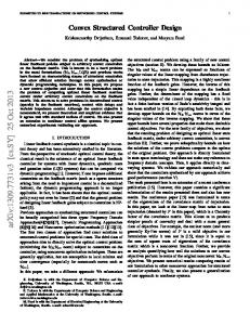
Figure 4.1: Uncertain system model time experiments the input-output behavior can be described with the help of a fictive n +n ×n +n +n disturbance d0 ∈ Ln2 d and by an LFT of a given LTI model U ∈ RH∞zu y wu d u and a structured dynamic uncertainty ∆0 in the form � � � � wu0 zu U11 U12 U13 = d0 , wu0 = ∆0 zu , (4.2) yˆ U21 U22 U23 u | {z } U
see also Figure 4.1. The unknown dynamics ∆0 ∈ S∆u belongs to a set of stable perturbations nw
S∆u = {∆ ∈ RHn∞wu ×nzu | ∆ = diag{∆1 , . . . , ∆τ }, ∆i ∈ RH∞ u,i
×nzu,i
, i = 1, ..., τ }(4.3)
n ×n
Block U23 ∈ RH∞y u is the nominal model, which can be the result of an identification method for restricted complexity models. Other blocks Uij describe the interconnection structure of the nominal model and the structured uncertainty. The uncertainty can be normalized by weighting functions nwu ×nwu W∆ = diag{W∆,1 Iwu,1 , . . . , W∆,τ Iwu,τ } ∈ RH∞
Wd = diag{w1 , . . . , wnd } ∈ RHn∞d ×nd
41
CHAPTER 4. UNCERTAINTY MODELLING AND ROBUST CONTROL DESIGN FOR LTI SYSTEMS such that for all ∆0 ∈ S∆u there exists a perturbation ∆ and for all d0 ∈ L2 there exists a normalized disturbance d such that ∆0 = W∆ ∆, d0 = Wd d,
∆ ∈ BS∆u ,
d ∈ BL2
The feedback signals wu := ∆zu = [wu,1 , ..., wu,τ ]T and zu = [zu,1 , ..., zu,τ ]T are partitioned according to block structure S∆u .
4.1.2
Experiments and model consistency
Information about the true system is gained by taking experiments: the system is excited by input signal u(t) which can be either a predefined signal (open-loop experiment) or the output of a controller (closed-loop experiment). The inputs and outputs of the true system are measured and stored. We assume that the sampling is fast enough to have a good sampled data representation of the signals, i.e., the Shannon conditions hold. Then, Discrete Fourier Transform (DFT) can be applied, possibly with a window function, to compute the frequency-domain representation of the signals. Many textbooks are dealing with the topic of sampling and Fourier transform, in the sequel we does not concern signal processing problems of this kind. Suppose that the input-output data of system T in the lth experiment are given ω }, where nω is the number of in the frequency domain by El = {(yl (jωk ), ul (jωk ))nk=1 S frequency samples. The data containing N experiments are denoted by E N = N l=1 El .
Definition 4.1 (Consistency) The uncertain system (4.2) with weighting functions W∆ and Wd is consistent with respect to data set El if the following condition holds. There exists a perturbation ∆l ∈ BS∆u and a disturbance dl ∈ BLn2 d such that measured output yl is exactly reproduced by model output yˆl , i.e., for all frequencies k = 1, ..., nω
(4.4)
yˆl (jωk ) = yl (jωk ) where yˆl (jωk ) := FU (U (jωk ), W∆ (jωk )∆l (jωk ))
�
Wd (jωk )dl (jωk ) ul (jωk )
�
The model is unfalsified if it is consistent with all experiments E N . It is required of the model structure to be able to represent the true system in all experiments. Certain rank conditions on system U , detailed in Section 4.2, ensure the satisfaction of Assumption 4.1 There exist a W∆ and a Wd such that the model is consistent with all experiments. 42
4.1. PROBLEM FORMULATION
z¯� p
GT
yK
� � �
d¯ r¯ uK
-
K
Figure 4.2: Closed-loop system configuration with true plant
4.1.3
Control performance
In modern control theory, the requirements on the control performance are defined by drawing the closed-loop control configuration. New inputs, outputs and weighting functions are introduced to build an augmented closed-loop system whose input-output mapping is to minimize in some chosen norm. In order to specify the objectives of the design, true system T is augmented and placed in a closed-loop configuration as in Figure 4.2. New inputs, denoted by r¯, containing known or measurable signals, e.g., reference inputs, can be added. Performance outputs, denoted by z¯p , which should be small during the control, must be defined. Signals yK and uK are defined as the inputs and outputs of controller K. They are not necessarily equal to y and u, respectively. Augmented plant GT contains system T and weighting functions, which specify performance signal z¯p and normalize outer signals r¯ ¯ and d. The control objective is to minimize γ¯ (K) :=
sup
¯ ¯,¯ T ∈ST ,d∈S d r ∈BL2
k¯ zp k2 ,
¯ r¯). z¯p = FL (GT , K)(d,
(4.5)
Since true plant T and sets ST and Sd¯ are not known in advance, the controller will be designed based on model (4.2) which must be augmented in the same way, resulting in augmented plant G0 and the configuration in Figure 4.3. Without loss in generality, system G0 and input r¯ can be scaled such that we can calculate with wpT := [dT r T ] ∈ BLn2 d +nr instead of d ∈ BLn2 d , r¯ ∈ BLn2 r . In order to minimize the control objective (4.5) by calculations based on model (4.2), we will need the following assumption on performance specification. Assumption 4.2 The consistency of the model (4.2) with respect to closed-loop data (yl (jωk ), ul (jωk )) implies of the augmented plant model in Figure 4.3 �� � � �� the consistency rl (jωk ) zp,l (jωk ) and that zp,l (jωk ) = z¯p,l (jωk ). , with respect to data uK,l (jωk ) yK,l (jωk ) Assumption 4.2 expresses that plant augmentation preserves the consistency property. We can summarize the problem statement as follows. Problem 1. Given an unknown system T , an LTI plant model U of fixed structure for uncertainty and control specification defined by G0 . Provide an iterative uncertainty model unfalsification and robust control design procedure that 1. constructs a consistent 43
CHAPTER 4. UNCERTAINTY MODELLING AND ROBUST CONTROL DESIGN FOR LTI SYSTEMS -
∆
zu
wu w � u0
z� p
G0
�d0
W∆ � Wd
� �
yK
�
d� wp r
uK -
K
Figure 4.3: Closed-loop system configuration with the model for robust control design model (U, W∆ , Wd ) for the true plant, based on closed-loop experiments, and 2. designs a H∞ controller K that minimizes objective (4.5).
4.2
Characterization of uncertainty
In this section all consistent models are parameterized with respect to given measurement data. The frequency-domain model validation technique and affine parametrization given in [123] are applied for the constant matrix problem at a certain frequency point. Then consistency constraints are defined for the normalizing weighting functions of the model. Consistency equation (4.4) is satisfied if and only if there exist wu0,l (jωk ) and d0,l (jωk ) solving � � � � wu0,l (jωk ) el (jωk ) = U21 (jωk ) U22 (jωk ) , d0,l (jωk )
where nominal model error is defined by el (jωk ) := yl (jωk ) − U23 (jωk )ul (jωk ). For solvability of the equation, the nominal model error must satisfy � � el (jωk ) ∈ Im{ U21 (jωk ) U22 (jωk ) }, which ensures the satisfaction of Assumption 4.1. In order to avoid trivial solutions dim(Ker[U21 (jωk ) U22 (jωk )]) > 0 is also assumed. In this case all solutions can be formalized as � � � � � �� � � �† wu0,l (jωk ) Bu (jωk ) el (jωk ) U21 (jωk ) U22 (jωk ) = , d0,l (jωk ) Bd (jωk ) θlk �
� � � Bu (jωk ) where forms a basis for the kernel of U21 (jωk ) U22 (jωk ) and θlk ∈ Bd (jωk ) Cnwu +nd −ny is any free parameter at frequency ωk and experiment l. The parametrization of weighting functions in W∆ and Wd can be given indirectly through parameters θlk and some inequality constraints as follows. 44
4.3. ROBUST PERFORMANCE CRITERION Theorem 4.1 Given stable and stable invertible weighting functions W∆ and Wd as defined in Section 4.1.1 and given the set E N of measurement data. Then, for every experiment l = 1, ..., N there exists a perturbation ∆l ∈ BS∆u and a disturbance dl ∈ BLn2 d that satisfy consistency condition (4.4) for all k and l, if and only if there exist θlk k = 1, ..., nω and l = 1, ..., N such that |wu0,l,i (jωk , θlk )| , i = 1, . . . , τ |zu,l,i (jωk , θlk )| |Wd,i (jωk )| ≥ |d0,l,i (jωk , θlk )| i = 1, . . . , nd
|W∆,i (jωk )| ≥
(4.6) (4.7)
The theorem follows from the results of [79, Lemma 3], [25] and [28]. The solutions W∆ and Wd of Problem 1 are characterized by set ΘN := {θlk ∈ Cnθ , l = 1, ..., N, k = 1, ..., nω } with nθ = nwu +nd −ny and constraints (4.6) and (4.7). Whenever parameters θlk are fixed, any low-order stable, stable invertible weighting functions W∆,i (jωk ) or Wd,i (jωk ) can be chosen that tightly over-bound in magnitude the right hand sides of (4.6) and (4.7), respectively. The weighting functions determined by the choice of parameters θlk , l = 1, ..., N , k = 1, ..., nω and the over-bounding method are denoted by W∆ (ΘN ) and Wd (ΘN ). For simplifying notation W := diag{W∆ , Wd , I} is introduced where the dimension of the unity matrix I depends on the context. The nominal closed-loop system M0 := FL (G0 , K), the weighted nominal closed-loop system M := M0 W and the weighted augmented plant G := G0 W are defined where W is of appropriate size. An uncertainty model which is consistent with experiments E N can be represented by W (ΘN ). For a simple example on the parametrization of weighting functions, see Section A.2 in Appendix A. The following section defines the robust performance measure which is a criterion for tuning the weighting functions and designing the controller.
4.3
Robust performance criterion
Worst case performance level γ¯ (K) defined on the true closed-loop system cannot be computed, since ST and Sd¯ are not known. A computable upper-bound of γ¯ (K) will be derived in this section based on model (4.2). Define the worst-case performance level based on the model as γ¯s (K, W ) :=
sup wp ∈BL2 ,∆∈BS∆u
kzp k2 =
sup ∆∈BS∆u
kFL (FU (G0 W, ∆), K)k∞ .
If the model is consistent with the true plant and Assumption 4.2 holds, then there exist wp ∈ BL2 , ∆ ∈ BS∆u for all T ∈ ST , d¯ ∈ Sd¯ such that zp = z¯p . As a result, we can conclude Lemma 4.1 If W is consistent with the data of all experiments with controller K, then γ¯s (K, W ) ≥ γ¯(K). 45
CHAPTER 4. UNCERTAINTY MODELLING AND ROBUST CONTROL DESIGN FOR LTI SYSTEMS Remark. 4.1 A more stringent statement also holds: If W is consistent with the data of an experiment, say El , generated in closed-loop by controller K, then γ¯s (K, W ) ≥ k¯ zp,l k2 . This is also a simple consequence of Assumption 4.2 and definition of γ¯s (K, W ). Clearly, we are interested in the smallest upper-bound denoted by γ¯s (K) := inf¯ γs (K, W ), sought among all consistent models. For the purpose of computing the robust performance of systems with consistent uncertainty models, the bounds for perturbations must be fixed to k∆k∞ ≤ 1, since the weighting functions capture the size information. The measure that scales only the performance channel is the skewed SSV introduced in Section 3.2. Given a controller K, the sought upper-bound of γ¯ (K) is γ¯s (K) := γ, where γ is the solution of the following optimization problem. min
D,W,γs (jω)
γ
(4.8)
subject to γ ≥ γs (jω),
∀ω
−1 (jω) W (jω) diag{γs (jω)Iwu , Ind +nr }) < γs (jω), σ ¯ (DL (jω) FL (G0 (jω), K(jω)) DR
where W satisfies (4.6) and (4.7) in all experiments with K and D, DL , DR are defined in Section 3.2. In the iterative algorithm presented in the next section, the theoretic consistency constraint on W must be replaced by the one based on a finite set of experiments performed so far. In each stage of the iteration new information on the system is gained by means of new closed-loop experiments with the actual controller. It turns out that a new experiment is always such that it either remains consistent with the actual model and holds the achieved (a priori) performance bound or has a worst performance, and in the same time, falsifies the uncertainty model. This fortunate property is due to the chosen criterion skew µ, since ∆ ∈ BS∆u is guaranteed by both consistency and the control design. This is justified by the following theorem: Theorem 4.2 Given experimental data set E N and a controller K N designed for the consistent model characterized by W (ΘN ). The guaranteed performance level skew µ is γ¯s (K N ). A new experiment is performed with the controller on the true system defined in (4.1). The gathered data set is EN +1 , and the realized performance γ¯ N +1 := k¯ zp,N +1 k2 . Then, the following implications hold. 1. W (ΘN ) is consistent with EN +1 =⇒ γ¯ N +1 ≤ γ¯s (K N ) 2. γ¯ N +1 > γ¯s (K N ) =⇒ W (ΘN ) is not consistent with EN +1 . Proof. The first implication follows from Lemma 4.1. For proving the second one, suppose, in contrast to the claim, that kzp,N +1 k2 > γ¯s (K N ) and W (ΘN ) is consistent with EN +1 . Then, there exists a parameter set ΘN +1 such that W (ΘN +1 ) = W (ΘN ) and, for all k = 1, ..., nω , yˆN +1 (jωk ) = yN +1 (jωk ). By Assumption 4.2, z¯p,N +1 (jωk ) = zp,N +1 (jωk ) also holds. But bound (4.8) guarantees for the model with W (ΘN ) that |zp,N +1 (jωk )| ≤ γs (jωk ) ≤ γ¯s (K N ), which contradicts the initial supposition. 46
4.4. AN ITERATIVE ALGORITHM FOR UNCERTAINTY MODELLING AND CONTROL DESIGN The first implication expresses that if a new experiment does not falsify the model with W (ΘN ), then the performance of the control is, as expected, below the guaranteed level γ¯s (K N ). The second implication states that if the realized performance in the new experiment exceeds the guaranteed level, then the model is necessarily falsified. Based on these statements the following suggestions can be offered. According to implication 2., the performance should be measured during experiments. A degradation of performance by an unacceptable level can, generally, be noticed before instability would damage the system. In this case the experiment should be halted and the measured data can be used to improve the model. Consistency of the model should always be checked after experiments. Note that both implications of the theorem holds with classical criterion µ only if β := µ∆a (M ) ≤ 1, and it provides a conservative performance measure if β < 1. The reason is that performance is guaranteed for ∆ ∈ β1 BS∆u . If β > 1, a valid model may destabilize the system or an experiment of poor performance may be consistent with the actual model.
4.4
An iterative algorithm for uncertainty modelling and control design
In the following iterative algorithm basically two aims of opposing directions are integrated. Aim 1. is to increase robustness based on new data by decreasing the set of unfalsified models (increasing uncertainty weighting functions), which implies the degradation of achievable performance. Aim 2. is to chose an optimal unfalsified model, thus minimizing the robust performance level. Actually, all steps in D-K-W iteration minimize the upper-bound (4.8) of performance criterion skew µ. The subsequent sections detail the steps of the algorithm.
Algorithm 1. A. Initialization B. D-K-W iteration 1) Scaled H∞ controller synthesis (K) 2) Optimization of uncertainty model (W ) 3) Skew µ analysis by finding scalings (D) C. Closed-loop experiments D. Update of the uncertainty model
Step A. Initialization Let N = 1. Initial data set E 1 may consist of open- and closed-loop experiment data. 1 = I. Construct initial uncertainty bounds W (Θ1 ). Let DL1 = I, DR 47
CHAPTER 4. UNCERTAINTY MODELLING AND ROBUST CONTROL DESIGN FOR LTI SYSTEMS
Step B. D-K-W iteration The following three steps are iterated until the improvement of performance level γ¯s (K N ) is less than a given number in the last iteration steps of a given number. During the iteration only the stable controller with improved performance is stored. For notational brevity index N is omitted. Step B1. Controller synthesis −1 . A scaled γ iteration is Let the generalized plant be denoted by GD := DL G0 W DR applied where in each step the solvability of kFL (GD diag{γIwu , I}, K)k∞ < γ is tested by searching for an appropriate controller. This is a bisection algorithm with standard H∞ controller synthesis problem for scaled plant GD diag{γIwu , I}.
Step B2. Optimization of the uncertainty model −1 , K) denote the generalized closed-loop model with scalings. Let MD := FL (DL G0 DR Let vik > 0, i = 1, ..., τ + nd , be the candidate magnitudes of the uncertainty weighting functions at frequency ωk
vik = |W∆,i (jωk )|,
vτ +i k = |Wd,i (jωk )|,
i = 1, ..., τ, i = 1, ..., nd ,
(4.9) (4.10)
and let VI,k = diag{v1k Iwu,1 , ..., vτ k Iwu,τ , vτ +1 k , ..., vτ +nd k , Ir }. For each frequency point ωk , k = 1, ..., nω , minimize γk subject to σ ¯ ( MD (jωk )VI,k diag{γk Iwu , Ind +nr } ) < γk , |wu0,l,i (jωk , θlk )| vik ≥ , i = 1, ..., τ, l = 1, ..., N |zu,l,i (jωk , θlk )| vτ +i k ≥ |d0,l,i (jωk , θlk )|, i = 1, ..., nd , l = 1, ..., N
(4.11) (4.12) (4.13)
in variables θlk , l = 1, ..., N , and vik , i = 1, ..., τ + nd . Then, point-wise bounds vik are over-bounded by stable minimal-phase transfer function by using e.g. the log-Chebychev magnitude design algorithm of the reference [12, fitmagfrd.m]. The orders of the transfer functions are increased until the fitted weighting functions, denoted by W , satisfy γs (jωk ) < εγk , k = 1, ..., nω , where ε > 1 is a given tolerance and
Z=
�
γs (jωk ) := ρ(Z22 (jωk ) − Z12 (jωk )∗ (Z11 (jωk ) − Iwu )−1 Z12 (jωk )), � Z11 Z12 ∗ := W ∗ MD MD W, ∗ Z22 Z12
For the existence of γs (jωk ), Z11 (jωk ) < Iwu must hold. To ensure this a weighting wf it (ωk ) := ρ(Z11 (jωk )) is applied in the fitting procedure in order to force higher accuracy at frequencies where ρ(Z11 (jωk )) is near to 1. 48
4.4. AN ITERATIVE ALGORITHM FOR UNCERTAINTY MODELLING AND CONTROL DESIGN Step B3. Skew µ analysis by finding the scalings Let M := FL (G0 W, K),
DL,k := diag{d1k Izu,1 , ..., dτ k Izu,τ , Iz },
DR,k := diag{d1k Iwu,1 , ..., dτ k Iwu,τ , Ind +nr }.
Minimize γk frequency-wise subject to −1 diag{γk Iwu , Ind +nr } ) < γk σ ¯ ( DL,k M (jωk )DR,k
in variables dik > 0, i = 1, ..., τ . This convex problem is equivalent to a generalized eigenvalue problem. Then, point-wise scalings dik are fitted in magnitude by stable, stable invertible transfer functions where the selection of order and the weighting of the fitting criterion are similar to those in the previous step.
Step C. Closed-loop experiments In reference [131] the iterative control design schemes are classified as stability assured (all experiments are stable), instability tolerant (all experiments are stable after an a priori known iteration number) and stability uncertain (all experiments are stable after an a priori unknown iteration number). It is shown in [131] that the first two properties can be achieved only if strict a priori assumptions are made on the system. The approaches based on ν-gap metric, provide schemes with guaranteed stability, but the system generating the data is not allowed to change its dynamics, i.e. set ST is a singleton. This is not the case in this chapter. We can, however, borrow the idea of Ref. [130] on handling instability and saturation. Assumption 4.3 Saturation levels U and Y can be defined such that, for all t, any i = 1, ..., nu and any j = 1, ..., ny , |ui (t)| > U or |yj (t)| > Y infer the degradation of the performance beyond a certain level c: k¯ zp k2 > c. Closed-loop experiments are carried out by monitoring the saturation conditions. As soon as one of them is satisfied, the possibly destabilizing controller (K N ) is switched off and, instead, a known stabilizing controller or control input is switched on for a period long enough for the transients to decay. After this period K N can be switched on again. Theorem 4.2 guarantees that data EN +1 of the experiment invalidates model W (ΘN ), the weighting functions will be increased and in the next iteration the robustness of the controller will be improved. Practically, it can be useful to perform the first few iterations on a high-fidelity simulator program, while there is chance for saturation.
Step D. Update of the uncertainty model The consistency of model W (ΘN ) with EN +1 is checked as follows. Solve the following optimization problem point-wise for each ωk . Let vik := |W∆,i (jωk )|, i = 1, ..., τ and 49
CHAPTER 4. UNCERTAINTY MODELLING AND ROBUST CONTROL DESIGN FOR LTI SYSTEMS vik := |Wd,i (jωk )|, i = 1, ..., nω . Minimize γk subject to |wu0,N +1,i (jωk , θN +1 k )| , i = 1, ..., τ, |zu,N +1,i (jωk , θN +1 k )| vτ +i k + γk ≥ |d0,N +1,i (jωk , θN +1 k )|, i = 1, ..., nd ,
vik + γk ≥
If for all k = 1, ..., nω γk ≤ 0 holds, then, the algorithm is finished with controller K N uncertainty model W (ΘN ) and performance level γ¯s (K N ). Otherwise, let W (ΘN +1 ) be constructed by the over-bounding method S presented in Step B2 of Algorithm 1 for points vik + max(0, γk ). Let E N +1 = E N EN +1 , N = N + 1, and continue from Step B.
4.5
Solutions with convex optimization
An important special case of uncertainty model structure is when U12 = 0 and U11 is block-diagonal or zero. In this case signal zu is independent on parameters θlk and, therefore, (4.6) and (4.7) define LMI constraints. To show this first suppose that U11 is block-diagonal, i.e., wu,i = ∆0,i zu,i zu,i = U11,i wu,i + U23,i u for i = 1, ..., τ . It follows that wu,i = ∆0,i (I − U11,i ∆0,i )−1 U23,i u. It has been assumed that ∆0 and U are stable systems, consequently, a new additive uncertainty block can be introduced without loss in generality: ∆0,i := ∆0,i (I − U11,i ∆0,i )−1 Hence U11 = 0 can be assumed.
d
?
Wd
y
�
w u0
d0 ?
?
U22
U21
?
+�
?
+�
wu W∆ �
zu ∆ � U13
U23 �
6
u
Figure 4.4: Additive uncertain system model
50
Let the particular solution of consistency equation (4.4) be denoted by � � � �† au,lk := U21 (jωk ) U22 (jωk ) el (jωk ) ad,lk
4.5. SOLUTIONS WITH CONVEX OPTIMIZATION Define real diagonal matrices Vk = diag{|W∆ (jωk )|, |Wd (jωk )|} ∈ Rnwu +nd ×nwu +nd ,
(4.14)
diagonal of complex vectors � � au,lk,1 au,lk,τ , ..., , ad,lk,1 , ..., ad,lk,nd ∈ Cnwu +nd ×τ +nd , Alk = diag |zu,l,1 (jωk )| |zu,l,τ (jωk )| and diagonal of complex matrices � � Bu,1 (jωk ) Bu,τ (jωk ) Blk = diag , ..., , Bd,1 (jωk ), ..., Bd,nd (jωk ) ∈ Cnwu +nd ×nθ (τ +nd ) , |zu,l,1 (jωk )| |zu,l,τ (jωk )| and let Θlk = diag{θlk , ..., θlk } ∈ Cnθ (τ +nd )×τ +nd be the τ + nd times repeated blockdiagonal matrix. The consistency conditions formulated in Theorem 4.1 are provided for the case of additive uncertainty structure of Figure 4.4 in the following theorem. Theorem 4.3 Given stable and stable invertible weighting functions W∆ and Wd as defined in Section 4.1.1 and given set E N of measurement data. Then, for every experiment l = 1, ..., N there exists a perturbation ∆l ∈ BS∆u and a disturbance dl ∈ BLn2 d that satisfy consistency condition (4.4) for all k and l, if and only if there exist θlk k = 1, ..., nω and l = 1, ..., N such that � � (Alk + Blk Θlk )∗ Vk2 ≥0 (4.15) Alk + Blk Θlk Inwu +nd In Step B2 of Algorithm 1, constraints (4.12) and (4.13) should be replaced by (4.15). Note that Vk defined by (4.14) is nothing but Vk = diag{v1k Iwu,1 , ..., vτ k Iwu,τ , vτ +1 , ..., vτ +nd },
(4.16)
where vik > 0 are the candidate magnitudes of the uncertainty weighting functions at frequency ωk . Recall that VI,k = diag{Vk , Ir } has already been defined in Step B2 of Section 4.4. Criterion (4.11) can always be rewritten to the complex LMI of the form � � Inw 2 M (jω )∗ 2 V V k I,k D I,k >0 γk2 Ind +nr (4.17) 2 MD (jωk )VI,k I
by applying Schur complement. Minimization of γk2 subject to constraints (4.15) and 2 and γ 2 . (4.17) is a generalized eigenvalue problem in variables θlk , vik k Step D of Algorithm 1 (update of the uncertainty model) gives also a convex problem. The consistency of model W (ΘN ) with EN +1 is checked as follows. Solve the following optimization problem point-wise for each ωk . Let vik := |W∆,i (jωk )|, i = 1, ..., τ and vik := |Wd,i (jωk )|, i = 1, ..., nd . Minimize γk subject to � � Vk2 + γk2 I (AN +1 k + BN +1 k ΘN +1 k )∗ ≥0 AN +1 k + BN +1 k ΘN +1 k Inwu +nd 51
CHAPTER 4. UNCERTAINTY MODELLING AND ROBUST CONTROL DESIGN FOR LTI SYSTEMS Finally, we can conceive theoretical conditions for the model based upper-bound γ¯s (K) being equal to the true performance level γ¯ (K). For avoiding exactness problems due to sampling, and for simplifying notation, the conditions are stated in terms of continuous-frequency representation. Suppose that experimental data consist of inputoutput pairs (y(jω), u(jω)), ω ∈ R, of the worst-case experiment ¯ r¯) = arg Ewc = {(y(jω), u(jω)) | (T , d,
sup
¯ ¯,¯ T ∈ST ,d∈S d r ∈BL2
k¯ zp k2 }
i.e. the measured performance of the worst-case experiment equals to γ¯ (K). Theorem 4.4 Given a controller K and closed-loop experimental data set El = Ewc generated by K. Suppose, the structured uncertainty has at most two blocks: ∆u S∆u with τ ≤ 2, and the uncertainty structure is additive, i.e., U11 = 0 and U12 = 0. Suppose that Assumption 4.2 holds. Then γ¯ (K) = max γ(ω) ω
where γ(ω) is the optimum of the following minimization problem: Minimize γ(ω) subject to (4.17) and (4.15), where all variables and transfer matrices are taken at ω instead of ωk . Proof. From τ ≤ 2 it follows that extended perturbation block ∆a in the robust performance problem has at most three complex blocks, which implies that µ upper-bound −1 ) = µ∆a (M ). Assumption 4.2 ensures that zp = z¯p which is exact: inf D σ ¯ (DL M DR implies that the calculated bound maxω γ(ω) is at least γ¯ (K), i.e. it is an upper-bound. However, this upper-bound is exact, since the additive structure allows a convex characterization of the optimization problem, for this reason there exist Θl and vi such that kzp k2 is the worst-case performance of the model. A simple illustrative example for the D-K-W iteration with standard (non-skew) µ-synthesis is presented in Appendix A.
Remarks on Algorithm 1 On model validation methods The measurement data define a set of consistency constraints on the uncertainty model. Time-domain model validation approaches, e.g. [108] and [124], have the drawback that they cannot handle long data series. This is because in case of dynamic uncertainty, the number of variables is at least as high as the length of the experiment. Frequencydomain methods [123, 25, 28] and [79] have the advantage that the problem reduces to a series of small tractable feasibility problems. The number of variables increases linearly with the number of experiments. A further problem arises from the structure of the uncertainty model. Structured uncertainty model in LFT interconnection leads to a model validation problem, which is a NP-hard problem in general. There are, however, many approaches for computing 52
4.5. SOLUTIONS WITH CONVEX OPTIMIZATION approximate solutions in the model validation context. Methods based on S-procedure [124, 98], scaling-approach [28] and skew µ approach [30, 73, 95] are some examples. In the latter approach, the model validation problem is reformulated as a skew µ analysis problem and there is no direct connection to the skew µ synthesis of the dissertation. Concerning control synthesis, the available robust design methods have their limits in case of too sophisticated uncertainty descriptions. The upper bounds on the SSV, in case of mixed parametric and dynamic uncertainties, are not necessarily tight [45, 89]. Based on the above discussion, the perturbation model in the dissertation is restricted to contain only LTI components. The special case of η(θ) = η is particularly advantageous in computational point of view, because the algorithm consists of only convex optimization steps subject to LMI constraints.
Implementation The controller synthesis step and the search for the scalings can be implemented by the minor modification of the existing routines in the Robust Control Toolbox for Matlab [12] designed for D-K iteration. The computational burden of steps D and K is the same as in the µ-synthesis. Step W requires approximately the same complexity of calculations as step D. We note that it is numerically more advantageous to introduce a variable for the last block of DL and DR , and the search for scalings is followed by a normalization step.
Generalization to other class of systems Frequency-domain consistency constraints are applicable in case of LTI perturbation models. Nominal model G23 , however, does not play a role in the constraints, it can be replaced, therefore, by LPV or nonlinear models. The only requirement is that a robust controller can be designed for the structured uncertainty model. A formulation of the algorithm for LPV nominal models is presented in Chapter 5. For the sake of simplicity the plant is restricted to be stable in the present work. This assumption is necessary for the used frequency-domain model validation method. The proposed scheme can be extended, however, to unstable systems along the idea presented in [54]. The extension can be the subject of future research.
Convergence of iterations Standard D-K iteration is not guaranteed to converge to the global optimum, but it has been shown to work on practical problems with LTI perturbations [99]. The same can be said about the presented D-K-W iteration [RGB09, RGB10, RG10]. Regarding the whole iterative algorithm, the uncertainty set increases with every new falsifying experimental data. In the presented applications (Sections 4.6, 5.6 and Chapter 6) the algorithm stopped after 2-3 iterations. 53
CHAPTER 4. UNCERTAINTY MODELLING AND ROBUST CONTROL DESIGN FOR LTI SYSTEMS
4.6
Case study: Active steering for vehicle stability enhancement - LTI case
The example of this section has been constructed to demonstrate the proposed iterative algorithm. A frequent problem in automotive control is to design a steering controller for yawrate reference tracking. This problem emerges for example when the objective is to improve ride quality and steerability by making the steering robust against variations in road conditions, wind effects and vehicle parameters (e.g. mass and load distribution) [85, 97, 103].
Figure 4.5: Concept of steering control In the presented example, the driver force on the steering column is manipulated by an additional motor drive mounted on the steering rack. The reference for the manipulation is generated by a reference model of the vehicle which produces a desired yaw-rate signal based on the measured steering-wheel angle (see Figure 4.5). The controller is to generate an additional steering force/angle to enforce the vehicle to track the yaw-rate reference while attenuating effects of road and wind. The only sensors used by the proposed control algorithm are yaw-rate and steering wheel angle which are available on commercial vehicles. The performance is defined in terms of L2 norm of the tracking error and the control signal. True system T consists of a linearized single-track model and a steering system dynamics plotted in Figures 4.6-4.7. They approximate the dynamics of a MAN/Actros heavy truck. The model equations can be derived based on [RB05a] and [Röd07]. The LTI system is given by the state-space description
T :
�
x˙ y
�
=
�
A Bd Bu C Dd Du
�
x d u
˙ R δm δ˙m ], disturbance d = v 2 , control input with state vector xT = [β ψ˙ δ δ˙ ∆R ∆ wind 54
4.6. CASE STUDY: ACTIVE STEERING FOR VEHICLE STABILITY ENHANCEMENT - LTI CASE ˙ The system matrices are given by u = Td and output y = ψ.
cf +cr mv cr lr −cf lf J z
A=
−
0
nRK cf Jsl
0 0 0 0
cr lr −cf lf mv 2 cr l2r +cf l2f − Jz v
cf mv c f lf Jz
−1 +
0
Ksl ǫ nRK cf lf Jsl + Jsl v
0
− MbǫR 0 0
0
−
Ksl +nRK cf Jsl
0
b MR
0 0
0
0
0
0
0
0 1
0 0
sl −B Jsl 0 0 0 0
Ksl NL Jsl
0 0 0 1
0 0 0 0
− RpaMR − NLbMR
a MR
0
BR −M R 0
0 0 0 0 0 1
CS Jsw Rp
km Jsw Rp
0
� � wβ � � 07×1 Bd = wr , Bu = , C = 0 1 01×6 , Dd = 0, 1 cJsw 06×1
0 S − JCsw
m − Jksw
Du = 0
The state and input variables are defined in Table 4.1 and the physical parameters in
Figure 4.6: Single-track model
Figure 4.7: Neglected dynamics: a stock steering system. Table 4.2. Adhesion coefficient µ and vehicle velocity v are constant uncertain parameters which define set ST : in each iteration of the algorithm, Step C consists of three experiments with (µ, v) ∈ {(0.2, 10), (1, 30), (1, 10)}. 55
CHAPTER 4. UNCERTAINTY MODELLING AND ROBUST CONTROL DESIGN FOR LTI SYSTEMS
Table 4.1: State and input variables β ψ˙ δ ∆R δm vwind Td
vehicle side-slip angle yaw-rate (measured output) steering angle rack position steering wheel angle side-wind velocity (disturbance) applied torque on the steering wheel (control input)
Table 4.2: Physical parameters of the vehicle model lf = 2.3444m, lr = 2.8056m m = 14200 kg cf = µ 2.5201 106 , cr = µ 1.9144 106 Jz = 123780 Nm/(rad/sec2) Jsw = 0.034 Nm/(rad/sec2) m Nm Ksc = 42700 N rad , Bsc = 0.36042 rad/s) m Nm Ktb = 83 N rad , Btb = 0.0 rad/s) MR = 6 kg Rp = 0.007367 m BR = 352 Nm/(rad/s) NL = 0.11816 m m Nm Ksl = 14878 N rad , Bsl = 160 rad/s) ǫ = 0.01 ηF = 0.985, ηβ = 0.985 ηps = 0.95 Gps = 30 N/rad Jsl = 6.1 Nm/(rad/sec2 ) nRK = 0.0061 m c = 0.0039 wβ = 0.0012, wr = 8.1435 ∗ 10−5 Ksc ∗Ktb Bsc ∗Ktb Cs = K , km = K sc +Ktb sc +Ktb Ksc ∗Gps Cs sl a = ηF Rp + ηps Ksc +Ktb , b = 2ηβ RK R NL µ = 1 (nominal) 0.2, 1, 1 (test) v = 15 (nominal) 10, 30, 10 m/s (test)
COG-front and COG-rear axis distances Mass of vehicle Front and rear cornering stiffness Inertia of vehicle around the vertical axis Inertia of steering wheel Steering column stiffness and damping Torsion bar stiffness and damping Mass of rack Radius of pinion Rack damping Steering linkage ration Steering linkage stiffness and damping Roll steer coefficient Efficiency of forwd./backwd. torque transmission Efficiency of power steering torque transmission Power steering gain Cumulative inertia of steering linkage and tire Total tire trail length Normalizing factor such that δ(∞) ≈ Td (∞) Wind force factors on slip and yaw-rate
Adhesion coefficient in experiment 1,2,3 Absolute velocity in experiment 1,2,3
The steering system dynamics is considered as unknown and the linearized singletrack model is used for control design. The nominal model is given by ˙ c +c c l −c l cf − fmv r −1 + r rmv2f f mv β β cr l2 +cf l2 cf lf ψ˙ ψ¨ = (4.18) Gn : cr lr −cf lf − rJz v f Jz Jz T ynom d 0 1 0 Based on Table 4.2, note that the input is scaled so that Td = δ in the nominal model. 56
4.6. CASE STUDY: ACTIVE STEERING FOR VEHICLE STABILITY ENHANCEMENT - LTI CASE r-
Tdriver
Wr
zu ?
∆
w-u
u = Td
+
ψ˙ ref
- Wref
W∆
wu0 ? -+ - G n
d? Wd d0
+ ? ˙ ? - + y = ψ- + -
6
z
�2
Wu �
uK = Tc
K �
yK
z1
- W t
Figure 4.8: Control specification: the closed-loop system with normalizing weighting functions. The nominal value of uncertain adhesion coefficient µ = 1 is built in cornering stiffness parameters (cf , cr ) and the nominal velocity is v = 15 m/s. The neglected steering system dynamics acts on the steering angle input of the nominal model, for this reason a natural choice for the uncertainty structure is input-multiplicative perturbation ∆0 = T Gn − 1 that belongs to set S∆u = {∆ ∈ RH∞ }. The effect of the side-wind is modelled by an additive disturbance on the system describing the structure of � � the output. Thus, 0 0 1 . the uncertainty will be U = Gn 1 Gn The goal of the control is given by the specification of the closed-loop system in Figure 4.8. Blocks ∆, W∆ , Gn and Wd constitute the uncertain system. The torque 75 of the driver on the steering wheel Tdriver drives reference model Wref = (s+5) 2 , which represents the required behavior of the vehicle. Block Wr normalizes physical signal Tdriver . Signal ψ˙ ref is to be followed by applying an additional torque Tc generated by feedback controller K. Tracking error ψ˙ ref − ψ˙ is penalized by low-pass filter Wt = s+3 in order to achieve good tracking at steady state and at low frequencies. 0.025 s+0.001 2
Control signal uK = Tc is penalized by high-pass filter Wu = 1.4 (s+0.04) in order to (s+10)2 avoid high-frequency components. Augmented plant mapping [wu0 | d0 r | uK ]T 7−→ [zu | z1 z2 | yK ]T is given by
0 −Wt Gn G0 = 0 −Gn
√ 0√ Wr / 2 1 √ −Wt / 2 Wt (Wref − Gn )Wr / 2 −Wt Gn 0√ 0 Wu √ −1/ 2 (Wref − Gn )Wr / 2 −Gn
,
√ where term 2 is incorporated in order to normalize input vector [d r]T . Initial data set E 1 is generated by three open-loop experiments associated with the three systems in ST . In all experiments (open- and closed-loop) the same driver torque Tdriver , plotted in Figure 4.11(c) (dash-dot), and the same side-wind velocity, plotted in Figure 4.9, will be applied. A sampling time of 0.01s is used and the frequency domain data is derived by discrete Fourier-transformation (DFT). 57
CHAPTER 4. UNCERTAINTY MODELLING AND ROBUST CONTROL DESIGN FOR LTI SYSTEMS Disturbance on the vehicle side wind velocity [m/s]
20
15
10
5 v
wind
0
0
10
20
30
40
50
60
70
80
90
time [s]
Figure 4.9: Side-wind velocity in the experiments. Disturbance weighting function |Wd|
Perturbation weighting function |W∆|
20
10
10
0 −10 magnitude, dB
magnitude, dB
0 −10 −20
−20 −30
−30 −40 −50
true sup|d| DK DKW 1 DKW 2 DKW 3 −2
10
−40 −50 0
10 frequency, rad/s
2
10
(a)
true sup|∆| DK DKW 1 DKW 2 DKW 3 −2
10
0
10 frequency, rad/s
2
10
(b)
Figure 4.10: Disturbance (a) and perturbation (b) weighting functions. True uncertainty (o), initial (DK), and subsequent iterations DKW 1, 2, 3. (Data at ω1 = 0 is ω2 = 7 ∗ 10−4 rad/s) plotted at 100 Given the control specifications, the first task is to chose initial weighting functions for the uncertainty. In this numerical example we can exactly calculate the boundaries of the multiplicative perturbation set as |W∆,true (jω)| = maxT ∈ST | GTn(jω) (jω) − 1|. Similarly, the maximal magnitude of the true additive disturbance can be calculated. These boundaries are plotted in Figure 4.10 by small ’o’ markers. It can be seen from Figure 4.10(b) that the size of the perturbation is greater than -6dB=0.5012 (minimum at ω = 0), i.e. the nominal model is very inaccurate. In the real problems, however, the boundary of the uncertainty set is not known. Assume, the initial weighting functions in the uncertainty model are set according to the following scene: Based on engineering 0 := 0.6, which is judgement constant 60% is assumed for the neglected dynamics, i.e. W∆ a quite good estimation - a bit overestimated at low frequencies and a bit underestimated at higher frequencies. In order to start from a correct (consistent) model the following procedure is applied for the determination of the disturbance weighting function. Using the model validation constraints of Section 4.2 the upper-bound of the disturbance weighting function is minimized for each data point in E 1 (open-loop data) min αlk θlk
58
4.6. CASE STUDY: ACTIVE STEERING FOR VEHICLE STABILITY ENHANCEMENT - LTI CASE subject to |wu0,l (jωk , θlk )| |zul (jωk )| ≥ |d0,l (jωk , θlk )|
0.6 ≥ αlk
for l = 1, ..., N and k = 1, ..., nω . Values αlk are, then, over-bounded by weighting function Wd0 which is shown in Figure 4.10 by dotted line. The controller designed by Algorithm 1 is initialized by the controller designed by the skew D-K iteration (steps B1 and B3 in Algorithm 1) for the initial model with Wd0 and 0 . This controller is denoted by K W∆ DK . The evaluation of the uncertainty weighting functions during Algorithm 1 is presented in Figure 4.10. After the first application of D-K-W iteration the size of perturbation decreases significantly to W∆ (Θ1 ), while that of the disturbance increases to Wd (Θ1 ) (dashed lines in Figure 4.10). This means that the weighting functions got farther from the true weighting functions: the neglected dynamics is modelled partly as an effect of disturbance. The resulting controller is denoted by KDKW,1 . Then, the three closed-loop simulations with KDKW,1 are carried out. Step D reveals that the new data invalidates the model. Thus, the iteration continues. After three iterations the analysis shows that data E 4 are consistent with the resulting uncertainty model, therefore, the algorithm stops. The reference-tracking and the control signals of KDK and the last controller KDKW,3 are plotted in Figures 4.11(a)-4.11(c). Among the three plants in ST the one with (µ, v) = (0.2, 10) is the worst-case showing the largest oscillations1 . This plant is destabilized by initial controller KDK : at about t = 43s the yaw-rate attains the predefined saturation level and uK = Tc is set to zero2 , meanwhile the yaw-rate converges to the open-loop case. At t = 53s controller KDK is switched on again and the yaw-rate starts to oscillate. Figure 4.11(b) show the yaw-rate of the final DKW controller for both the worst-case plant with (µ, v) = (0.2, 10) and for the case with (µ, v) = (1, 30). Despite the large uncertainty the final controller achieved good tracking performance for all plants in the set. ˙ The L2 -norm of the tracking error, kψ˙ ref (t) − ψ(t)k 2 , is also computed during the simulations. The norm is plotted in Figure 4.11(d), showing the superiority of the DKW controllers over KDK . Regarding each controller, Table 4.3 shows the achieved robust performance level γ¯s (K) and the satisfaction of the consistency conditions based on the closed-loop simulation data. Table 4.3: Performance levels of the controllers γ¯s (K) consistency
KDK 0.2234 ×
KDKW,1 0.1595 ×
KDKW,2 0.2035 ×
KDKW,3 0.1980 X
1
Only the experiments with parameter setting (µ, v) = (0.2, 10) are plotted in Figures 4.11(a)-4.11(c) Applied steering torque Td became equal to driver torque Tdriver in period t ∈ [43s, 53s], see Figure 4.11(c). 2
59
CHAPTER 4. UNCERTAINTY MODELLING AND ROBUST CONTROL DESIGN FOR LTI SYSTEMS Figure 4.10 show that the weighting functions represent the size and shape of a fictive uncertainty set that serves for a mathematical description (or rather inclusion) of the true system. They values depend on the control specification, not on the true system. It can be seen that uncertainty modelling improved the guaranteed performance. Controller KDKW,1 after the first iteration is the best performing controller, however, it is designed based on an invalid model. In the subsequent iterations the robustness of the controllers is increased. The final controller is consistent with all measurements. Reference tracking with the final KDKW
Reference tracking with K=0 and with KDK, (µ,v)=(0.2,10)
0.6
1.5
0.4
1
yaw−rate, rad/s
yaw−rate, rad/s
0.2 0.5 0 −0.5 −1 −1.5 −2 0
rref open−loop KDK 20
0 −0.2 −0.4 −0.6
rref
−0.8
KDKW,3, (µ,v)=(0.2,10) KDKW,3, (µ,v)=(1,30)
−1 40 time, s
60
0
80
10
(a)
20 time, s
30
40
(b) Tracking performance of the controllers
Control signals Td with (µ,v)=(0.2,10)
5 K
DK
0.2 0 −0.2 −0.4
T
driver
K
−0.6
Norm of the tracking errors
Steering torque, Nm
0.4
4
KDKW,1 KDKW,2 K
3
DKW,3
2
1
DK
KDKW,3 −0.8 0
20
40 time, s
(c)
60
80
0 0
20
40 time, s
60
80
(d)
Figure 4.11: Simulation results (a) - yaw-rate reference ψ˙ ref (solid), open-loop response (dash-dot), closed-loop response with KDK (dotted). (b) - yaw-rate with final controller KDKW,3 in two experiments. (c) - control signals: driver torque Tdriver (dash-dot), Td with KDK (dotted), with KDKW,3 (solid). (d) - evaluation of reference tracking error ˙ kψ˙ ref (t) − ψ(t)k 2 (sum of the three experiments)
60
4.7. SUMMARY AND THESIS 1
4.7
Summary and Thesis 1
In this chapter, a design algorithm for weighting functions characterizing structured uncertainty is developed. It is based on frequency-domain model validation results by Smith and Doyle [123], but consistency conditions are utilized in an optimization problem as constraints where the objective is to tune the weighting functions in order to minimize a control performance criterion. This weight optimization problem is placed into an iterative experimenting, unfalsification and robust control design framework. No a priori information is assumed on the true system that generates experiment data. It is only assumed that the true system is stable and in every experiment it can be modelled by a given LTI nominal model with LFT interconnection to structured dynamic perturbations and disturbances. The objective is to minimize the robust performance of the true controlled system by designing both the weighting functions and the controller. It is shown that if the model is consistent with all experiment data that can be obtained with a given controller, then an upper-bound of the true performance can be computed based on the model (Lemma 4.1). The lemma suggests the idea of using closed-loop experiments to falsify/unfalsify models, and thus improve the consistency of the model. In fact, one cannot do more than just improving robustness when no a priori information is available on the bounds of uncertainty. Guarantee cannot be given for stability and performance. It is proved, furthermore, in Theorem 4.2 that, when using a control synthesis method developed for minimizing skew µ criterion, then the following statements hold: • if a model is not falsified by a new experiment, then the actual performance of the control is, as expected, below the guaranteed level • if the realized performance in the new experiment exceeds the guaranteed level, then the model is necessarily falsified Based on these implications a stability uncertain (defined by [130]) iterative scheme can be proposed where instability is detected in time and measurement data is utilized for improving robustness of the controller. The proposed scheme is summarized in Algorithm 1 where details of skew µ-synthesis and weighting function design are elaborated. Finally, a class of uncertainty structures are defined which turns the steps of the algorithm into convex problems which can be solved based on LMIs. The contribution of this chapter can be summarized in the following thesis: Thesis 1 An iterative algorithm has been elaborated for LTI models with the aim of shaping structured uncertainty models and designing robust controllers based on measurement data. The algorithm handles unstable experiments ensuring safe improvement of guaranteed robust performance on the true, unknown system. For additive uncertainty structures, the algorithm is formulated as a series of LMI problems. The steps of skew µ synthesis 61
CHAPTER 4. UNCERTAINTY MODELLING AND ROBUST CONTROL DESIGN FOR LTI SYSTEMS has been elaborated as part of the algorithm. It has been proved that performance degradation beyond the guaranteed level implies falsification of the actual model, which forces the continuation of the algorithm. Own publications related to the chapter and thesis: [RB05b, RB06b, RB06a, RGSB08, Röd09, RBar, RG10].
62
Chapter 5
Uncertainty modelling and robust control design for LPV systems The class of LPV systems has become more important in the last two decades due to its modelling power for nonlinear/time-varying systems and the quick development in the related control theory. Many analysis and synthesis results have been successfully inherited from the LTI system’s theory, as it is shown e.g. by the unified framework of Chapter 3, and the adapted popular control methods: LQG control and Kalman-filtering [134], [RBL02], fault detection and isolation [11], model predictive control [105], and so on. This line is continued in the chapter: iterative uncertainty modelling and robust control design method is elaborated for LPV systems with LFT scheduling parameter dependence and structured dynamic uncertainty. The design of robust LPV controllers based on intuitive choice of weighting functions is an even more time-consuming and laborious iterative task than in case of LTI controllers. The surplus labour is due to the increased computational burden of controller synthesis and the additional design parameters related to LPV modelling (e.g. choice of scheduling variables and its polytope). The automated and control oriented design of uncertainty weighting functions may drastically decrease the design effort while improving robust performance. In the iterative algorithm presented in Chapter 4, a frequency-domain consistency constraint is applied for the reason of computational advantages. The linearity of nominal model U23 is not utilized in the uncertainty modelling step of Algorithm 1, even the nominal model does not play a role there. In fact, the nominal model can be of any class of systems. One important property we require of the algorithm is that criterion for uncertainty modelling and control design are the same. This means that the system class of the nominal model must be such that control criterion (robust performance) can be characterized in the frequency-domain. This requirement is fulfilled in case of LPV systems with LFT parametrization of the scheduling variables. The modelling and the analysis are carried out in the frequency-domain and the LPV control design is performed in the time-domain. Analysis and synthesis of LPV systems are carried out via multipliers and IQCs. The relation between µ analysis and IQCs is formulated in Section 5.2. Controller synthesis method for uncertain LPV systems with LFT parameter dependence is discussed in 63
CHAPTER 5. UNCERTAINTY MODELLING AND ROBUST CONTROL DESIGN FOR LPV SYSTEMS Section 5.3. The uncertainty modelling criterion and constraints are presented in Section 5.4. The joint uncertainty modelling and control design algorithm for LPV systems is summarized in Section 5.5. The efficiency of the method is demonstrated on the vehicle steering problem in Section 5.6.
5.1
Problem formulation
The true plant to be controlled and which generates the data is described by (4.1). Suppose that in finite time experiments its input-output behavior can be described with the help of a fictive disturbance d0 ∈ Ln2 d and by an LFT of a given LPV model and a structured dynamic uncertainty ∆u0 in the form �
zu yˆ
�
=
� |
U11 U21
wu0 U12 U13 d0 , wu0 = ∆u0 zu , U22 U23 (∆s ) u {z } �
(5.1)
U
where U23 (∆s ) is an ny × nu LPV nominal model with LFT dependence on scheduling parameter ∆s ∈ S∆s , where S∆s is defined by (3.31). Other blocks Uij , ij 6= 23 belong to RH∞ and describe the interconnection structure of the nominal model and structured dynamic uncertainty, ∆u0 ∈ S∆u , where S∆u is defined by (4.3). Normalizing weighting functions, W∆ , Wd , are stable LTI systems such that ∆u0 = W∆ ∆u , ∆u ∈ BS∆u and d0 = Wd d, d ∈ BL2 . Suppose that the input-output data of system T in the lth experiment are given in the S frequency domain as El . The data containing N experiments are denoted by EN = N l=1 El . The consistency definition in Section 4.1 still holds with the modification that transfer function U (jωk ) does not exists, U being an LPV system, but model output yˆ can be transformed to the frequency-domain by DFT. The control objective is to minimize (4.5), where controller K = K(∆s ) is allowed to depend on the on-line measurable scheduling parameter via LFT. An upper-bound can be calculated for γ¯ (K(∆s )) based on a consistent model in the same way as described in Chapter 5. To this end the control performance is specified on the model, as well, by augmenting U , as described in Section 4.1, and so, the system configuration plotted in Figure 5.1 is obtained. It is also supposed that assumptions 4.1 and 4.2 hold. The assumptions allow the existence of unfalsified uncertainty models and the establishment of consistency based on generalized plant G0 . We can summarize the problem statement as follows. Problem 2. Given an unknown system T , a plant model U and control specification defined by G0 . Provide an iterative uncertainty model unfalsification and robust control design procedure that 1. constructs a consistent model (U, W∆ , Wd ) for the true plant, based on closed-loop experiments, and 2. designs an LPV controller K(∆s ) that minimizes objective (4.5). 64
5.2. RELATION BETWEEN SKEW µ ANALYSIS AND IQC APPROACH -
∆u
zu
wu -
∆s
zs
w � u0
W∆ �
ws
�
G0
zp �
�du0 � �
yK -
Wd
�
d r
uK
K
wc
zc ∆c
�
Figure 5.1: Closed-loop system configuration with the LPV model
5.2
Relation between skew µ analysis and IQC approach
It is shown in this section that abstract performance characterization with appropriate multipliers leads to the same upper-bounds as in the (skew) µ-analysis. In this way, performance characterization used for LTI systems in Chapter 4 is adopted into the IQC framework, which is the tool of analysis and synthesis of LPV systems. In this section, the scheduling parameter dependence is disregarded temporarily, and the uncertain system in Figure 3.2 � is considered� where ∆ ∈ S∆u represents a structured Mu Mup dynamic perturbation and M = denotes a LTI system. Mpu Mp It is easy to verify that IQC (3.8) with parametrization Qω (jω) = −γDr (jω)∗ Dr (jω), Sω (jω) = 0, Rω (jω) = γ −1 Dl (jω)∗ Dl (jω),
Dr := diag{d1 Iw∆1 , ..., dτ Iw∆τ },
Dl := diag{d1 Iz∆1 , ..., dτ Iz∆τ }, di , d−1 i ∈ RH∞ , i = 1, ..., τ
implies σ ¯ (∆) ≤ γ −1 . Quadratic performance specification (3.7) with (3.10) and (3.11) is equivalent to � �∗ � � Z ∞ 1 I I ∗ wp (jω) Pp wp (jω)dω ≤ −εkwp k22 M∆ (jω) M∆ (jω) 2π −∞ by applying Parseval-theorem and inserting zp = M∆ wp , where M∆ = FU (M, ∆) is the uncertain closed-loop system. When Pp is defined by (3.11) and (3.12), the latter IQC leads to quadratic constraint ∗ −1 −γp I + M∆ γp M∆ < 0,
65
CHAPTER 5. UNCERTAINTY MODELLING AND ROBUST CONTROL DESIGN FOR LPV SYSTEMS by Lemma 2.2. This implies that σ ¯ (M∆ ) < γp , i.e., the L2 gain of the uncertain system is at most γp . Condition (3.9) of robust performance reappears as ∗ w∆ 0 0 −γDr∗ Dr 0 w∆ � � Z ∞ −1 D ∗ D z∆ z∆ 1 0 γ 0 0 w l ∆ l dω ≤ −ǫk k22 wp 0 0 −γp I 0 wp 2π −∞ wp zp zp 0 γp−1 I 0 0 which is equivalent to ∗ 0 −γDr∗ Dr I 0 −1 D ∗ D Mu Mup 0 γ l l 0 0 0 I 0 0 Mpu Mp
0 0 I 0 Mu Mup 0 0 −γp I 0 0 I 0 γp−1 I Mpu Mp
0 and multiplier Pa with (3.32)-(3.33) satisfying (5.4) if and only if there exist X, Y and multipliers Ps ∈ SP and P˜s ∈ SP˜ that satisfy the LMIs � � Y I (5.7) > 0, , ΓTX PX ΓX < 0, ΓTY PY ΓY > 0, I X where
PX
=
ΓX
=
PY
=
0 0 0 0 −I 0 0 0 Qs 0 0 0 X 0 0 0 0 0 0 0 SsT 0 0 0
0 0 0 Qp 0 0 0 SpT
X 0 0 0 0 0 0 0
I 0 0 0 0 I 0 0 0 0 I 0 0 0 0 I e e e e A Bu Bs Bp e eu D e us D e up Cu D es D e su D es D e sp C e e e ep Cp Dpu Dps D
0 0 0 0 Y 0 0 0
0 0 0 −I 0 0 es 0 0 Q ep 0 0 Q 0 0 0 0 0 0 T e 0 Ss 0 0 0 SepT
Y 0 0 0 0 0 0 0
0 0 0 0 0 0 0 Ss 0 0 0 Sp 0 0 0 I 0 0 0 Rs 0 0 0 Rp
Υ
0 0 0 0 0 0 0 Ses 0 0 0 Sep 0 0 0 I 0 0 es 0 0 R ep 0 0 R
73
CHAPTER 5. UNCERTAINTY MODELLING AND ROBUST CONTROL DESIGN FOR LPV SYSTEMS
ΓY
=
eT −A euT −B esT −B epT −B I 0 0 0
euT −C esT −C epT −C T T T e u −D e su −D e pu −D T T e us e sT −D e ps −D −D T T e up e sp e pT −D −D −D 0 0 0 I 0 0 0 I 0 0 0 I
Φ
Since uncertainty is present, the output-feedback controller synthesis for robust performance problem is a non-convex optimization problem, as discussed in Section 3.3. One approach is to solve the optimization by iteration using both (5.7) and (5.5). In one step, the scalings related to the dynamic uncertainty are designed in the frequency-domain: point-wise search over a frequency grid followed by fitting the magnitude of a stable minimum-phase transfer function. In a second step, the fitted scalings are connected to system G to build system GaD for which a nominal LPV controller is designed as described in Section 3.4. The algorithm is extended by the design of uncertainty weighting functions, and the complete procedure is placed in the iterative uncertainty modelling and control design algorithm as discussed in the next sections.
5.4
Optimizing the uncertainty model
The goal of this section is to extend the conditions of robust performance of uncertain LPV systems by model consistency conditions in order to simultaneously test consistency and performance. When a scalar performance level is defined, then an optimization problem can be formulated in the uncertainty model parameters. By this means an unfalsified uncertainty model can be tuned in order to tighten the upper-bound of robust performance. According to Theorem 5.1 robust quadratic performance is satisfied if (5.5) holds. In the proof of the theorem, it is shown that (5.5) is equivalent to the frequency domain inequality (5.6). In order to connect consistency and control performance conditions, inequality (5.6) has to be reformulated as a function of uncertainty model parameters vik , i = 1, ..., τ + nd defined by (4.9)-(4.10), which are parameters of consistency constraints (4.12)-(4.13) as well. We derive results for the special case of additive uncertainty, discussed in Section 4.5, because this leads to an LMI problem. The general case follows from this result by simply replacing the LMI associated with the consistency constraints by general constraints (4.12)-(4.13). By pulling out the weighting functions related to the uncertainty model, scaled unweighted closed-loop nominal system MD0 is defined by MD = MD0 W
with W = diag{W∆ , Iws +wc , Wd , Inr }
As in Section 4.5, define uncertainty weighting function magnitude parameters vik , i = 1, ..., τ + nd , constituting the diagonal matrix Vk as in (4.14) and (4.16) and define 74
5.4. OPTIMIZING THE UNCERTAINTY MODEL VIk := |W (jωk )|, k = 1, ..., nω . Then, W (jωk ) can be factorized as W (jωk ) = VIk Ω(jωk ), where Ω(jωk ) = diag{Ω∆ (jωk ), Iws +wc , Ωd (jωk ), Inr } is a unity amplitude diagonal phase function with Ω(jωk )∗ = Ω(jωk )−1 . Introduce the following real matrices for simplifying notation of the multiplier in (5.6): QD = diag{−I, Qa , Qp } SD = diag{0, Sa , Sp }
RD = diag{I, Ra , Rp } At frequency points ω = ωk , (5.6) is equivalent to �� �∗ � � � I QD S D I