JovianDATA: A Multidimensional Database for the Cloud Sandeep Akinapelli Satya Ramachandran
[email protected] [email protected] Bharat Rane Ravi Shetye Vipul Agrawal
[email protected] [email protected] [email protected] Anupam Singh Shrividya Upadhya
[email protected] [email protected]
Abstract The JovianDATA MDX engine is a data processing engine, designed specifically for managing multidimensional datasets spanning several terabytes. Implementing a terascale, native multidimensional database engine has required us to invent new ways of loading the data, partitioning the data in multi-dimensional space and an MDX (MultiDimensional eXpressions) query compiler capable of transforming MDX queries onto this native, multidimensional data model. The ever growing demand for analytics on huge amount of data needs to embrace distributed technologies such as cloud computing to efficiently fulfill the requirements. This paper provides an overview of the architecture of massively parallel, shared nothing implementation of a multidimensional database on the cloud environment. We highlight our innovations in 3 specific areas - dynamic cloud provisioning to build data cube over a massive dataset, techniques such as replication to help improve the overall performance and key isolation on dynamically provisioned nodes to improve performance. The query engine using these innovations exploits the ability of the cloud computing to provide on demand computing resources.
1
Introduction
Over the last few decades, traditional database systems have made tremendous strides in managing large datasets in relational form. Traditional players like Oracle[7], IBM[14] and Microsoft[4] have developed sophisticated optimizers which use both shared nothing and shared disk architectures to break performance barriers on terabytes of data. New players in the database arena - Aster Data (now TeraData)[8], Green Plum (now EM C 2 )[2] - have taken relational performance to the petabyte scale by applying the principles of shared nothing computation on large scale commodity clusters. 17th International Conference on Management of Data COMAD 2011, Bangalore, India, December 19–21, 2011 c
Computer Society of India, 2011
For multi-dimensional databases, there are 2 prevalent architectures[6]. The first one is native storage of multi-dimensional objects like Hyperion Essbase (now Oracle)[15] and SAS MDDB[3]. When native multidimensional databases are faced with terabytes or petabytes of data, the second architecture is to translate MDX queries to SQL queries on relational systems like Oracle[13], Microsoft SQL Server or IBM DB2[14]. In this paper, we illustrate a third architecture where Multi-Dimensional Database is built on top of transient computing resources. The JovianDATA multi-dimensional database is architected for processing MDX queries on the Amazon Web Services (AWS) platform. Services like AWS are also known in the industry by the buzzword Cloud Computing. Cloud Computing provides tremendous flexibility in provisioning hundreds of nodes within minutes. With such unlimited power come new challenges that are distinct from those in statically provisioned data processing systems. The timing and length of resource usage is important because most cloud computing platforms charge for the resources by the hour. Too many permanent resources would lead to runaway costs in large systems. The placement of resources is important because it is naive to simply add computing power to a cluster and expect query performance to improve. This leads us to 3 important questions. When should resources be added to a big data solution? How many of these resources should be maintained permanently? Where should these resources be added in the stack? Most database systems today are designed for linear scalability where computing resources are generally scaled up. The cloud computing platform calls for intermittent scalability where resources go up and down. Consider the JovianDATA MDX engine usage pattern. In a typical day, our load subsystem could use 20 nodes to materialize expensive portions of a data cube for a couple of hours. Once materialized, the partially materialized cube could be moved into a query cluster that is 5 times smaller i.e. 4 nodes. If a query slows down, the query subsystem could autonomically add a couple of nodes when it sees that some partitions are slowing down queries. To main-
Country State City Year MonthDayImpressions USA CALIFORNIA SAN FRANCISCO2009 JAN 12 43 USA TEXAS HOUSTON 2009 JUN 3 33 . . . USA WASHINGTON WASHINGTON 2009 DEC 10 16
Table 1: Base table AdImpressions for a data warehouse tain this fluidity of resources, we have had to reinvent our approach to materialization, optimization and manageability. We achieve materialization performance by allocating scores of nodes for a short period of time. In query optimization, our focus is on building new copies of data that can be exploited for parallelism. For manageability, our primary design goal is to identify the data value combination that are slowing down the queries so that when nodes are added, load balancing of the partition housing these combination can happen appropriately. Specifically, we will describe 3 innovations in the area of processing multi-dimensional data on the cloud:1) Partition Management for Low Cost. On the cloud, nodes can be added and removed within minutes. We found that node addition or removal needs to go hand-in-hand with optimal redistribution of data. Blindly adding partitions or clones of partitions without taking into account query performance would mean little or no benefit with node addition. The partition manager in JovianDATA creates different tiers of partitions which may or may not be attached to an active computing resource. 2) Replication to improve Query Performance. In a cloud computing environment, resources should be added to fix specific problems. Our system continuously monitors the partitions that are degrading query performance. Such partitions are automatically replicated for higher degree of parallelism. 3) Materialization with Intermittent Scalability. We exploit the cloud’s ability to provision hundreds of nodes to materialize the most expensive portions of a multidimensional cube using an inordinately high number of computing nodes. If a specific portion of data (key) is suspected in query slowdown, we dynamically provision new resources for that key and pre-materialize some query results for that key.
2
Representing and Querying Multidimensional Data
The query language used in our system is the MDX language. MDX and XMLA (XML for Analysis) are the well known standards for querying and sending the multidimensional data. For more details about MDX, please refer to [12]. During the execution of an MDX query in the system, the query processor may need to make several calls to the underlying store to retrieve the data from the warehouse. Design and complexity of the data structures which carries this information from query processor to the store is crucial to the overall efficiency of the system. We use a proprietary tuple set model for accessing the multidimensional data from the store. The query processor
Figure 1: Dimensions in the simple fact table sends one or more query tuples and receives one or more intersections in the form of result tuples. For illustration purposes, we use the following simple cube schema from the table 1. Example: In an online advertising firm’s data warehouse, Data are collected under the scheme AdImpressions(Country, State, City, Year, Month, Day, Impression). The base table which holds the impression records is shown in table 1. Each row in the table signifies the number of impression of a particular advertisement recorded in a given geographical region at a given date. The column Impression denotes the number of impressions recorded for a given combination of date and region. This table is also called as the fact table in data warehousing terminology. The cube AdImpressions has two dimensions: Geography, Time. The dimensions and the hierarchy are shown in the figure 1. Geography dimension has three levels: country, state and city. Time dimension has three levels: year, month and day. We have one measure in the cube called impressions. We refer to this cube schema throughout this paper to explain various concepts. 2.1
Tuple representation
The object model of our system is based on the data structure, we call as ‘tuple’. This is similar to the tuple used in MDX notation, with a few proprietary extensions and enhancements. A tuple consists of set of dimensions and for each dimension, it contains the list of levels. Each level contains one of the 3 following values. 1) An ‘ALL’, indicating that this level has to be aggregated. 2).MEMBERS value indicating all distinct values in this level 3) A string value indicating a particular member of this level. Our system contains a tuple API, which exposes several functions for manipulating the tuples. These include setting a value to level, setting a level value to aggregate, Crossjoining with other tuples etc. 2.1.1
Basic Query
We will explain the tuple structure by taking an example of a simple MDX query shown in query 1. The query processor will generate the tupleset shown below for evaluating query 1. Note that, the measures are not mentioned explicitly, because in a single access we can fetch all the measure values. An setting for a particular level indicates that the corresponding level has to be aggregated. Even though the query doesn’t explicitly mention about the aggregation
on these levels, it can be inferred from the query and the default values of the dimensions. SELECT {[Measures].[Impressions]} ON COLUMNS ,{ ( [Geography].[All Geographys].[USA] ,[Time].[All Times].[2007] ) } ON ROWS FROM [Admpressions]
Query 1: Simple tuple query Country USA
2.1.2
State City Year Month ALL ALL 2007 ALL Query tupleset for Query 1
Day ALL
Descendants operator will be resolved by the compiler at the compile time and will be converted to the above tuple notation. The first tuple in the tuple set represents all the states in the country ‘USA’. The second tuple represents all the cities of all the states for the country ‘USA’. We use several other complex notations, to represent query tuples of greater complexity. E.g., queries that contain MDX functions like Filter(), Generate() etc. In the interest of the scope of this paper, those details are intentionally omitted.
3
Basic Children Query
Query 2 specifies that the MDX results should display all the children for the state ‘CALIFORNIA’ of country ‘USA’, for the june 2007 time period on the rows. According to the dimensional hierarchy, this will show all the cities of the state ‘CALIFORNIA’. The corresponding tuple set representation is shown below.
Architecture
The figure 2 depicts the high level architecture of the JovianDATA MDX engine. In this section, we give a brief introduction about the various components of the architecture. More detailed discussion of individual components will appear in subsequent sections.
SELECT {[Measures].[Impressions]} ON COLUMNS ,{ ( [Geography].[All Geographys].[USA].[CALIFORNIA].children ,[Time].[All Times].[2007].[June] ) } ON ROWS FROM [AdImpressions]
Query 2: Query with children on Geography dimension Country USA
State City Year CALIFORNIA .MEMBERS 2007 Query tupleset for Query 2
Month June
Day ALL
As described above, .MEMBERS in the City level indicates that all the distinct members of City level are needed in the results. After processing this tuple set, the store will return several multidimensional result tuples containing all the states in the country ‘USA’. 2.1.3
Basic Descendants Query
Query 3 asks for all the Descendants of the country ‘USA’, viz. all the states in the country ‘USA’ and all the cities of the corresponding states.The corresponding tuple set representation is shown below. SELECT {[Measures].[Impressions]} ON COLUMNS ,{ Descendants ( [Geography].[All Geographys].[USA] ,[CITY] ,SELF AND BEFORE ) } ON ROWS FROM [AdImpressions]
Query 3: Query with descendants on Geography dimension Country USA USA
State City Year .MEMBERS ALL ALL .MEMBERS .MEMBERS ALL Query tupleset for Query 3
Month ALL ALL
Day ALL ALL
Figure 2: JovianDATA high level architecture The query processor of our system consists of parser, query plan generator and query optimizer with a transformation framework. The parser accepts a textual representation of a query, transforms it into a parse tree, and then passes the tree to the query plan generator. The transformation framework is rule-based. This module scans through query tree and compresses the tree as needed, and converts the portions of tree to internal tuple representation and proprietary operators. After the transformation, a new query tree is generated. A query plan is generated from this transformed query tree. The query processor executes the query according to the compressed plan. During the lifetime of a query, query process may need to send multiple tuple requests to the access layer. The tuple access API, access protocols, storage module and the metadata manager constitutes the access layer of our system. The query processor uses the tupleset notation described in the previous section, to communicate with the access layer. The access layer accepts a set of query tuples and returns a set of result tuples. The result tuples typically contain the individual intersections of different dimensions. The access layer uses the access protocols to resolve the set
of tuples. It uses the assistance of metadata manager to resolve certain combinations. The access layer then instructs the storage module to fetch the data from the underlying partitions. A typical deployment in our system consists of several commodity nodes. Broadly these nodes can be classified into one of the three categories. Customer facing/User interface nodes: These nodes will take the input from an MDX GUI front end. These node hosts the web services through which user submits the requests and receives the responses. A Master node: This node accepts the incoming MDX queries and responds with XMLA results for the given MDX query. Data nodes: There will be one or more data nodes in the deployment. These nodes will host several partitions of the data. These nodes typically wait for the command from the storage module, processes them and returns the results back.
4
Data Model
In this section we discuss the storage and data model of our core engine. The basic component of the storage module in our architecture is a partition. After building the data cube, it is split into several partitions and stored in the cluster. Every partition is hosted by one or more of the data nodes of the system. In a typical warehouse environment, the amount of data accesses by the MDX query is small compared to the size of the whole cube. By carefully exploiting this behavior, we can achieve the desired performance by intelligently partitioning the data across several nodes. Our partition techniques are dictated by the query behavior and the cloud computing environment. In order to distribute the cube into shared nothing partitions, we have several choices with respect to the granularity of the data. The three approaches[6] that are widely used are, • Fact Table: Store the data in a denormalized fact table[10]. Using the classic star schema methodology, all multi-dimensional queries will run a join across the required dimensional table. • Fully Materialized: Compute the entire cube and stored in a shared nothing manner. Even though computing the cube might be feasible using hundreds of nodes in the cloud, the storage costs will be prohibitive based on the size of the fully materialized cube.
Country State City Year MonthDayImpressions USA CALIFORNIASAN FRANCISCO2009 JAN 12 43 USA TEXAS HOUSTON 2009 JUN 3 33
Table 2: Sample fact table The JovianDATA system takes the approach of materialized tuples rather than materialized views. In the next section, we describe the storage module of our system. For illustration purposes, we assume the following input data of the fact table as defined in table 2. We use query 1 and 2 from the section 2 for evaluating our model. Functionally, our store consists of dimensions. Dimensions consist of levels arranged in a pre-defined hierarchical ordering. Figure 1 show examples of the ‘GEOGRAPHY’ and ‘TIME’ dimensions. A special dimension called ‘MEASURES’ contains levels that are not ordered in any form. An example level value within the ‘MEASURES’ dimension is ‘IMPRESSIONS’. Level values within the ‘MEASURES’ dimension can be aggregated across rows using a predefined formula. For the ‘IMPRESSIONS’ measure level, this formula is simple addition. Among all the columns in fact table, only selected subset of columns are aggregated. The motive behind the partial aggregated columns will be elaborated more in further sections. This set of dimension levels, which are to be aggregated are called Expensive levels and the others as cheap (or non-expensive) levels. When choosing levels that are to be aggregated, our system looks at the distribution of data in the system, and does not bring in explicit assumptions about aggregations that will be asked by queries executing on the system. Competing systems will choose partially aggregated levels based on expected incoming queries - we find that these systems are hard to maintain if query patterns change, whereas our data based approach with hash partitioning leads to consistently good performance on all queries. For illustrative purposes, consider ‘YEAR’ and ‘STATE’ as aggregation levels for the following 9 input lines. If incoming rows are in the form of (YEAR, MONTH, COUNTRY, STATE, IMPRESSIONS) as shown in table 3 then the correponding table after partial aggreagtion is as shown in table 4. Year 2007 2007 2007 2007 2007 2007 2007 2007 2007
Month JAN JAN JAN JAN JAN FEB FEB FEB FEB
Country USA USA USA USA USA USA USA USA USA
State CALIFORNIA CALIFORNIA CALIFORNIA CALIFORNIA CALIFORNIA TEXAS TEXAS TEXAS TEXAS
Impressions 3 1 1 1 1 10 1 1 1
Table 3: Pre-aggregated Fact Table • Materialized Views: Create materialized views using cost or usage as a metric for view selection[9]. Materialized views are query dependent and hence cannot become a generic solution without administrative overhead.
Note that we have aggregated dimension-levels that we deem to be expensive and not aggregated other dimension levels. In many cases, for terabytes of data, we observed that the size of the partially aggregated cube ends up being smaller than the size of the input data itself.
Year 2007 2007 ALL ALL ALL ALL 2007 2007
Month JAN FEB JAN FEB JAN FEB JAN FEB
Country USA USA USA USA USA USA USA USA
State CALIFORNIA TEXAS CALIFORNIA TEXAS ALL ALL ALL ALL
Impressions 7 13 7 13 7 13 7 13
user query contains either ‘*’ or ‘value’ in each of the aggregate levels. • Cheap (Slow) Dimension Statistics: – Distinct value: Queries which involves Distinct value in the children query involves selecting one row from the slow dimension table
Table 4: Partially-aggregated Cube 4.1
Cheap dimension levels helps in compressing the cube in two ways. Firstly, by not aggregating these levels, multiple aggregation combinations will be avoided, thus keeping the cube size low. Secondly, since these levels are not aggregated, for every combination of expensive dimensions, the slow dimension combinations are limited, but repeated. This redundancy in the slow dimension combinations can be exploited by isolating the slow dimension combinations into a separate table, and using the identifiers to re-construct the original rows. In this technique, we split the cube data vertically, and create an identifier table or what we call cheap dimension table. Thus for the cube shown in table 4 the cube and the cheap dimension table formed after vertical decomposition are shown in table 5 and table 6 respectively. Year 2007 2007 ALL ALL ALL ALL 2007 2007
State CALIFORNIA TEXAS CALIFORNIA TEXAS ALL ALL ALL ALL
CheapDimId ID 1 ID 2 ID 1 ID 2 ID 1 ID 2 ID 1 ID 2
Impressions 7 13 7 13 7 13 7 13
Table 5: Partially-aggregated Cube with CheapDimId CheapDimId ID 1 ID 2
Month JAN FEB
Country USA USA
Table 6: Cheap Dimension Table
4.2
– Aggregate Value: Queries which involves aggregate in children levels, needs to perform aggregation on the entire slow dimension table in worst case.
Cheap dimensions storage model
Selecting Expensive dimension levels
Partial aggregation plays key role in our cube subsystem. Out of n columns in the fact table, m columns will be marked as expensive columns. Remaining (n-m) columns will be marked as non-expensive. The division is based on the empirical observation of the time bounds of different set of configurations and following factors. The storage model for expensive and non-expensive dimension is motivated to provide the faster response times for expensive keys in the tuple. The partition table is partitioned vertically, using expensive and non-expensive columns. The row relationships are maintained by encoding each slow dimension level’s unique combination. This storage structure, along with the aggregation scheme influences the choice of expensive dimensions and non-expensive dimensions. The following are some of the key factors which affect the choice. The
• Expensive (Fast) (Dim)ension Statistics – Expensive (Fast) Dim combination size : For certain combinations of the expensive dimensions, the selectivities of the slow dimension combinations are lower, which leads to processing of more rows. – Expensive (Fast) Dim per-partition Key cardinality: This involves how many keys are packed in a single partition or single node. As more keys are packed in a single node, the access time increases. – Expensive (Fast) Dim Avg per-key size: We use the following criteria to bifurcate the dimension set into expensive and non expensive dimensions. 1. Cube compression: If the number of distinct values in a dimension is small, the number of different combination it produces is much smaller. This results in a compact cube. 2. Cube explosion: If there are multiple dimensions listed as expensive, some dimensions are more likely to produce exponential set of cube rows. This is called as expression selectivity, and is a key factor in determining the expensive dimensions. 3. Slow dimension table size: Since the slow dimensions are maintained in a separate table, as the more number of slow dimensions participate, The size of this table grows. Once we have partially materialized the tuples, we partition them using the expensive dimensions as the keys for partitioning. In the next section, we show how these partitions are managed. 4.3
Partition Manager
The JovianDATA storage system manages its partitions across different tiers of storage. The storage tiers are used to maintain the Service Level Agreements at a per partition level and also to achieve the desired performance levels. The outline of the storage system is shown in the figure 3. There are 5 different states for an individual partition
load state is generally represented by a temporary EC2 compute node. Temporary EC2 nodes are deployed to generate cube lattices or update existing lattices of the cube. • Replicate: A partition is in the replicate state when the partition’s data is hosted on multiple nodes. The primary goal for partition to move into replicated state is to improve parallelism of a single query. In the figure above, the Partition P2 has been identified for replication and is hosted on 5 different hosts. In Amazon Web Services, a partition in replicated state exists with different copies residing on different EC2 compute nodes. Temporary EC2 nodes might be deployed to host replicas of a partition. Figure 3: Partition states in the storage • Archived: A partition is in the Archived state when the data is stored in a medium that cannot be used to resolve queries. In other words, the data in archived partitions is not immediately accessible for querying. To make an archived partition available for queries or updates, the archived partition has to be promoted to the operational state. In the figure above, the partition P3 is in archived stage. A partition is moved to the archival stage if the partition manager detects that partition is not being used for queries or updates. Of course, there is a cost to bringing a partition to ‘life’. The challenge is to identify the partitions that are needed in archival storage. In Amazon Web Services, the archival storage is the S3 buckets. Every partition is stored as an S3 bucket. • Operational: A partition is in the Operational state when the partition’s data can be used for resolution of a tuple. All tuple resolution occurs on the CPU of the node which owns the partition. The operational state is the minimum state for a partition to be usable in a query. A partition in operational state cannot be used for updates. A partition in operational state can be promoted to the load state or to the replication state. In the figure above, the partitions P1 and P2 are in the operational state. These partitions can be used to directly resolve tuples for incoming queries. In Amazon Web Services, the operational partition’s owner is an EC2 compute node. An EC2 node is a virtual machine with a disk attached to it. When query comes in and a tuple is located on an operational partition, any late aggregations are performed on the EC2 node that owns the partition. • Load: A partition is in the Load state when the partition’s data can be used for incremental updates or for a ‘first time’ load. No tuples can be resolved on these systems. A partition in the load state can be transitioned to archive storage before it can become operational. In Amazon Web Services, a partition in a
• Isolated A partition is in the materialized state when a partition’s keys have been isolated and fully materialized. Partitions are moved into this state when the ‘last minute’ aggregations are taking too much time. 4.4
Cost Based Partition Management
The partition manager’s ability to divide partitions into Archived, Operational, Load, Replicate and Isolate categories allows for a system which uniquely exploits the cloud. Each state has a different cost profile • Archived: An archived partition has almost zero cost because it resides on a secondary storage mechanism like S3 which is not charged by the hour. We try to keep the least access partition in the archived state. • Operational: Partitions in operational state are expensive because they are attached to actual nodes which are being charged by the hour on the cloud platform. • Load: Partitions in load state are expensive for really short periods of time where tuple materialization might require a high number of nodes. • Replication: Partitions in Replication state are more expensive than operational partitions as each replica is hosted on a separate node. In the replicated access protocol section, we explain the selection criteria for moving a partition into the replicated state. • Isolated: Isolated keys are the most expensive because they have dedicated hosts for single keys. In Isolation Based Access Protocol (IBAP) section, we explain the selection criteria for moving a key into an isolated partition state. The cloud environment presents the unique opportunity to dynamically add or remove the nodes based on the number of partitions that are in various states. The cost of maintaining a data processing system is the function over the cost of each state multiplied by the number of partitions in each state. When working with a large number of partitions
(more than 10,000), the cost of a system can be brought up or down simply by moving a few partitions from one state to another. 4.5
Distributing and querying data
We partition the input data based on a hash key calculated on the expensive dimension level values. So, all rows with a YEAR value of ‘2007’ and a STATE value of ‘TEXAS’ will reside in the same partition. Similarly, all rows with (YEAR, STATE) set to (‘2007’, ALL) will reside in the same partition. We will see how this helps the query system below. Note that we are hashing on ‘ALL’ values also. This is unlike existing database solutions[5] where hashing happens on the level values in input data rows. We hash on the level values in materialized data rows. This helps us create a more uniform set of partitions. These partitions are stored in a distributed manner across a large scale distributed cluster of nodes. If the query tuple contains ‘*’ on the cheap dimension levels, we need to perform an aggregation. However, that aggregation is performed only on a small subset of the data, and all of that data is contained within a single partition. If multiple tuples are being requested, we can trivially run these requests in parallel on our shared nothing infrastructure, because individual tuple requests have no inter-dependencies and only require a single partition to run against.
5
Access protocols
An access protocol is a mechanism by which our system resolves an incoming request in access layer. We have observed that the response time of the access layer is greatly improved by employing multiple techniques for different type of incoming tuples. For e.g., tuples which require a lot of computing resources are materialized during load time. Some tuples are resolved through replicas while others are resolved through special type of partitions which contain a single, expensive key. 5.0.1
On Demand Access Protocol (ODAP)
We classify On Demand Access Protocols as multidimensional tuple data structures that are created at run time, based on queries, which are slowing down. Here, the architecture is such that the access path structures are not updated, recoverable or maintained by the load sub system. In many cases, a ‘first’ query might be punished rather than maintaining the data structures. The data structures are created at query time after the compiler decides that the queries will benefit from said data structures. ODAP data structures are characterized by the low cost of maintenance because they get immediately invalidated by new data and are never backed up. There is a perceived cost of rematerializing these data structures but these might be outweighed by the cost of maintaining these data structures.
5.0.2
Load Time Access Protocol (LTAP)
We classify Load Time Access Protocols as multidimensional tuple data structures that are created and maintained as a first class data object. The classical LTAP is B-Tree data structure. Within this, we can classify these as OLTP(OnLine Transaction Processing) data structures and OLAP(OnLine Analytical Processing) data structures. OLTP data structures heavy concurrency and granular updates. OLAP data structures might be updated ’once-aday’. LTAP data structures are characterized by the high cost of maintenance because these data structures are usually created, as a part of the load process. These structure also need to be backed up (like any data rows),during backup process. Any incremental load should either update/rebuild these structures. 5.0.3
Replication Based Access Protocol (RBAP)
We have observed that the time required for data retrieval for a given MDX query is dominated by the response time of the largest partition the MDX query needs to accesses. Also in Multi Processing environment the frequently used partitions prove to be a bottle-neck with requests from multiple MDX queries being queued up at a single partition.To reduce time spent on a partition, we simply replicate them. The new replicas are moved to their own computing resources or on nodes which have smaller partitions. For eg. Partition which contains ‘ALL’ value in all the expensive dimensions is the largest partition in a materialized cube. So any query which has the query tupleset containing set of query tuples being resolved by this partition will have a large response time due to this bottle neck partition. In absence of replicas all the query tuples needed to be serviced by this partition line up on the single node which has the copy of that partition. This leads to time requirement upperbounded by Number of Tuples * Max. Time for single tuple scan. However if we have replicas of the partition, we can split the tuple set into smaller sub. sets and execute them in parallel on different replicas. This enables the incoming requests to be distributed across several nodes. This would bring down the retrieval time atleast to Number of Tuples * Max. Time for single tuple scan / Number of Replicas. When we implement RBAP we have to answer question like, ”How many partitions to replicate?”. If we replicate less number of partitions we are restricting the class of queries which will be benefitted from the new access protocol. Replicating all the data is also not feasible. Also while replicating we have to maintain the load across the nodes and make sure that no nodes get punished in the process of replication. Conventional data warehouses generally use replication for availability. Newer implementations of big data processing apply the same replication factor across the entire file system. We use automatic replication to improve query performance. The RBAP protocol works as follows:
1. After receiving the query tuples, group the tuples based on their HashValue. 2. Based on HashValue to Partition mapping, enumerate the partition that can resolve these tuples. 3. For each partition, enumerate the hosts which can access this partition. If the partition is replicated, the system has to choose the hosts which should be accessed to resolve the HashValue group. 4. We split the tuple list belonging to this HashValue group, uniformly across all these hosts, there by dividing the load across multiple nodes. 5. Each replica thus shares equal amount of work. By enabling RBAP for a partition, all replica nodes can be utilized to answer a particular tuple set. By following RBAP, we can ideally get performance improvement by a factor which is equal to the number of replicas present. Empirically we have observed a 3X improvement in execution times on a 5 node cluster with 10 largest partitions being replicated 5 times. We determine the number of partitions to replicate by locating the knee of the curve formed by plotting the partition sizes in decreasing order. To find the knee we use the concept of minimum Radius of Curvature (R.O.C.)as described by Weisstein in [16]. We pick the point where the R.O.C. is minimum as the knee point and the corresponding x-value as the number of partitions to be replicated. The formulae for R.O.C. we used is R.O.C. = y 00 /(1 + (y 0 )2 )1.5 Example: Consider the MDX query 4 and its query tuple set SELECT {[Measures].[Impressions]} ON COLUMNS ,{ ,[Time].[All Times].[2008].Children } ON ROWS FROM [Admpressions] WHERE [Geography].[All Geographys].[USA].[California]
Query 4: Query with children on Time dimension TupleID T1 T2 T3 T4 T5 T6 T7 T8 T9 T10 T11 T12
Year Month Country 2008 1 United States 2008 2 United States 2008 3 United States 2008 4 United States 2008 5 United States 2008 6 United States 2008 7 United States 2008 8 United States 2008 9 United States 2008 10 United States 2008 11 United States 2008 12 United States Query tupleset for Query 4
State California California California California California California California California California California California California
All the query tuples from the above tupleset have the same expensive dimension combination of year = 2008 ; state = California. This implies a single partition services all the query tuples. Say the corresponding partition which hosts the data corresponding to fast dimension year = 2008 ; state = California is Partition P9986 and in absence of replicas, let the lone copy be present on host H1 . In this
scenario all the 12 query tuples will line up at H1 to get the required data. Consider a scan required to a single query tuple require maximum time t1 secs. Now H1 services each query tuple in a serial manner. So the time required for it to do so is bounded by t1 * 12. Now let us consider RBAP in action. First we will replicate the partition P9986 on multiple hosts say H2 , H3 and H4 . Now partition P9986 has replicas on H1 , H2 , H3 and H4 . Let a replica of Partition Pj on host Hi be indicated by the pair (Pj , Hi ). Once the query tupleset is grouped by their Expensive Dimension combination the engine realises that the above 12 query tuples belong to the same group. After an Expensive Dimension - Partition look up the engine determines that this group of query tuple can be serviced by partition P9986 . A further Partition-Host look up determines that P9986 resides on H1 , H2 , H3 and H4 . Multiple query tuples in the group and multiple replicas of the corresponding partition, make this group eligible for RBAP. So the scheduler now divides the query tuples amongst the replicas present. So T1 , T5 and T9 are serviced by (P9986 ,H1 ), T2 , T6 and T10 are serviced by (P9986 ,H2 ), T3 , T7 and T11 are serviced by (P9986 ,H3 ) and T4 , T8 and T12 are serviced by (P9986 ,H4 ). Due to this access path we now bounded the time required to retrieve the required data to t1 * 3. So by following RBAP, we can ideally get performance improvement by a factor which is equal to the number of replicas present. A crucial problem which needs to be answered while replicating partitions is , ‘Which partitions to replicate?’. An unduly quick decision would declare that partition as the size metric. The greater the size of the partition, the greater its chances of being a bottleneck partition. But this conception is not true, since a partition containing 5000 Expensive Dimensions (ED) combinations each contributing to 10 rows in the partition will require lesser response time than a partition containing 5 ED combinations with each expensive dimension tuple contributing to 10000 rows. So the problem drills down to identifying partitions containing ED combination which lead to the bottle neck. Let us term such ED combinations as hot-keys. Apart from the knee function described above, we identify the tuples that contribute to the final result for frequent queries. Take for example a customer scenario where the queries were sliced upon the popular states of New York, California and Florida. These individual queries worked fine, but queries with [United States].children took considerable more time than expected. On detail analysis of the hot-keys we realised that the top ten bottle neck keys were No. 1 2 3 4 5 6 7 8 9 10
CRCVALUE 3203797998 1898291741 1585743898 2063595533 2116561249 187842549 7291686 605303601 83518864 545330567
SITE SECTION DAY COUNTRY NAME * * * * * 256 * * 256 * * * NO DATA * * NO DATA * 256 * * * * * 256 * * 256 * * * Top ten bottle-neck partitions
STATE * * * * * * VA VA MD MD
DMA * * 13 13 * * * * * *
Before running the hot key analysis, we were expecting ED combinations 1, 2, 3, 4, 5, 6 to show up. But ED com-
bination 7, 8, 9,10 provided great insights to the customer. It shows a lot of traffic being generated from the state of VA and MD. So after replicating the partitions which contain these hot keys and then enabling RBAP we achieved a 3 times performance gain. The next question we must answer is, ‘Does RBAP help every-time?’ The answer to this question is - No, RBAP deteriorates performance in the case where the serial execution is lesser than parallelization overhead. Consider a low cardinality query which would be similar to Query 4 but choose a geographical region other than USA, Calfornia, eg. Afganistan. Suppose this query returns just 2 rows. then it does not make sense to distribute the data retrieval process for this query. So to follow RBAP the query tuple set must satisfy the following requirements 1) The query tuple set must consist of multiple query tuples having the same ED combination and hence targeting the same partition. 2) The partition which is targeted by the query tuples must be replicated on multiple hosts. 3) The ED targeted must be a hot key. 5.0.4
Isolation Based Access Protocol (IBAP)
In cases where replication does not help, we found that the system is serialized on a single key within the system. A single key might be used to satisfy multiple tuples. For such cases, we simply move the key into its own single key partition. The single key partition is then moved to its own host. This isolation helps tuple resolution to be executed on its own computing resources without blocking other tuple access.
6
Performance
In this section we start with evaluating the performance of different access layer steps. We then evaluate the performance of our system against a customer query load. We are not aware of any commercial implementations of MDX engines which handles 1 TB of cube data hence we are not able to contrast our results with other approaches. For evaluating this query load, we use two datasets; a small data set and a large data set. The sizes of the small cube and large cube are 106 MB and 1.1 TB respectively. The configuration of the two different cubes we use, are described in table 7. The configuration of the data node is as follows. Every node has 1.7 GB of memory, 160 GB of local instance storage running on 32-bit platform having a CPU capacity equivalent to 1.2 GHz 2007 Opteron. 6.1
Cost of the cluster
The right choice of the expensive and cheap levels, depends on the cost of the queries in each of the models. Selecting the right set of expensive dimensions is equivalent to choosing the optimum set of Materialize Views which is know to be a NP hard problem[11], hence we use empirical observations and data distribution statistics and set of heuristics to determine the set of expensive dimensions.
The cloud system we use offers different types of commodity machines for allocation. In this section, we will explain the dollar cost of executing a query in the cluster with and without our architecture. The cost of each of these nodes with different configurations is shown in table 8. Metric Number of rows in input data Input data size (in MB) Number of rows in cube Cube size (in MB) Number of dimensions Total levels in the fact table Number of expensive levels Number of partitions Number of data nodes in the deployment
small cube 10,000 6.13 454,877 106.7 16 44 11 30 2
large cube 1,274,787,409 818,440 4,387,906,870 1,145,320 16 44 11 5000 20
Table 7: Data sizes used in performance evaluation Number of data nodes 5 10 20 50 100
Cost of the cluster ($s per day) High Memory instances High CPU Instances XL XXL XXXXL M XL 60 144 288 20.4 81.6 120 288 576 40.8 163.2 240 576 1152 81.6 326.4 600 1440 2880 204 816 1200 2880 5760 408 1632
Table 8: Cluster costs with different configurations The high memory instances have 160GB, 850GB, 1690 GB of storage respectively. Clusters which hold cubes of bigger sizes need to go for high memory instances. The types of instances we plan to use in the cluster may also influence the choice of expensive and cheap dimensions. In this section we contrast our approach with the Relational Group By approach. We use the above cost model to evaluate the total cost of the two approaches. Let us consider query 5 on the above mentioned schema and evaluate the cost requirement of both the model. SELECT { [Measures].[Paid Impressions] } ON COLUMNS ,Hierarchize ( [Geography].[All Geographys] ) ON ROWS FROM [Engagement Cube]
Query 5: Query with Hierarchize operator Firstly we evaluate the cost for our model, then for the relational Group-by model[1] followed by a comparision of the two. We took a very liberal approach in evaluating the performance of SQL approach. We assumed the data size, which can result after applying suitable encoding techniques. We created all the necessary indices, and made sure all the optimizations are in place. The cost of the query 5 is 40 seconds in the 5-node system with high memory instances. The cost of such a cluster is 144$ per day, for the 5 nodes. During load time we use 100 extra nodes, which will live upto 6 hours. Thus the temporary resources accounts to 720$. If the cluster is up and running for a single day the cost of the cluster is 864$ per day. For 2,3,5,10 and 30 days the cost of the deployment will be 504, 384, 288, 216, 168$ per day respectively.
Query
Cost for JovianDATA model of query 5 Let us assume a naive system with no materialized views. This system has the raw data partitioned into 5000 tables. Each node will host as many partitions as allowed by the storage. The cost for individual group by query is on a partition is 4 sec. To achieve the desired 40 seconds, number of partitions node can host are 40/4 =10 Number of nodes required = 5000/10 = 500 Cost of the cluster(assuming low memory instances) = 500*12 = 6000$.
1 2 3 4 5 6 7 8 9 10 11 12 13 14 15 16 17 18
Cost for Relational World model of query 5 The ratio of the relational approach to our approach is 6000/144 = 41:1 Assuming the very best of a materialized view, in which we need to process only 25% of the data, The cost of the cluster is 6000/4 = 1500$, which is still 10 times more than our approach.
JovianDATA Vs. Relational Model cost comparision for Query 5 Similar comparision was done for query 6 which costs 27s in our system.
Number of calculated measures 3 47 1 1 1 1 243 27 5 5 5 5 5 5 5 4 4 4
Number of intersections for small cube
Number of intersections for large cube
231 3619 77 77 77 77 243 81 5 5 5 5 290 15 160 12 4 4
231 3619 77 77 77 77 243 108 5 5 5 5 300 15 1370 12 4 4
Table 9: Queryset used in performance evaluation SELECT { Measures.[Paid Impressions] } ON COLUMNS ,Hierarchize ( [Geography].[All Geographys].[United States] ) ON ROWS FROM [Engagement Cube]
Query 6: Country level Hierarchize query The average cost for individual group by query is on a partition is 1.5 sec (after creating the necessary indices and optimizations). For 27 secs, number of partitions node can host are 27/1.5 =18 Number of nodes required = 5000/18 = 278 Cost of the cluster(with low memory instances) = 278*12 = 3336$. The ratio of relational approach to our approach is 3336/144 = 23:1 Assuming a materialized view, which needs only 25% of the data, The cost of the cluster is 3336/4 = 834$, which is still 6 times more than our approach.
JovianDATA Vs. Relational Model cost comparision for Query 6 6.2
Query performance
In this section, we evaluate the end-to-end performance of our system on a real world query load. The customer query load we use, consists of 18 different MDX queries. The complexity of the queries varies from moderate to heavy calculations involving Filter(), Sum(), Topcount() etc. Some of the queries involves calculated members, which performs complex operations like Crossjoin(), Filter() and Sum() on the context tuple. The structure of those queries are shown in table 9. We have run these queries against the two cubes described in previous section. The figure 4 shows the query completion times for the 18 queries against the small cube. The timings for the large cube are shown in figure 5. The X-axis shows the query id and the Y-axis shows the wall clock time for completing the query, in seconds. Each query involves several access layer calls throughout the execution. The time taken for a query depends on the complexity of the query and the number of separate access layer calls it needs to make. As evident from the figures, the average query response time for the small cube is 2 seconds. The average query response time for the large cube is 20 seconds. Our system scales linearly even though the data has increased by
Figure 4: Comparison of query timings for small cube 10,000 folds. The fact that the most of the queries are answered in sub-minute time frame for the large cube, is an important factor in assessing the scalability of our system. Note that, the number of intersections in the large dataset is higher for certain queries, when compared to that of smaller dataset. Query 15 is one such query where the number of intersections in large dataset is 1370, compared to 160 of the small dataset. Even though the number of intersections is more and the amount of data that needs to be processed is more, the response time is almost the same in both the cases. The distribution of the data across several nodes and computation of the result in a sharednothing manner are the most important factors in achieving this. To an extent, we can observe the variance in the query response times, by varying the number of nodes. We will explore this in the next section. 6.3
Dynamic Provisioning
As described in previous sections, every data node hosts one or more partitions. Our architecture stores equal number of partitions in each of the data nodes. The distribution of the partitions a tupleset will access is fairly random. If two tuples can be answered by two partitions belonging to the same node, they are scheduled sequentially for the completion. Hence by increasing the number of data nodes in
Figure 7: Comparison of timings with/without RBAP Figure 5: Comparison of query timings for large cube
Figure 8: Comparison of timings with/without key isolation Figure 6: Comparison of query time with varying number of nodes the deployment, the number of distinct partitions held by a node is reduced. This will result in reduction of the query processing time, for moderate to complex queries. This will also enables us to run number of queries in parallel, without degrading the performance much. We used an extended version of the queryset described in previous section generated by slicing and dicing. The figure 6 shows the graph of the query times by varying the number of nodes. The X axis shows the number of data nodes in the cluster. The Y axis shows the query completion time for all the queries. As evident from the figure, as the number of nodes is increased, the total time required for the execution of the query set is decreased. This will enable us to add more nodes, depending on the level of requirement. 6.4
Benefits of Replication
In this section, we take the query set and ran the experiments with/without replication. A replication enabled system will have an exactly 1 replica of every partition, distributed across several nodes. Our replication techniques ensure that a replica partition p0 of the original partition plies in a different node than the node, where original partition belongs to. This is crucial to achieve greater degree of parallelism. The figure 7 plots the time consumed by the individual queries. It contrast the imporvements, after enabling RBAP. The timings shown here are the wall clock times measured before and after enabling RBAP. By enabling RBAP, we have gained an overall improvement of
30% compared to the single partition store. The amount of time savings depends on the access pattern of the queries. The access patterns that are skewed will benefit the most, where as the other queries will get a marginal benefit. 6.5
Benefits of key isolation
From our experiments we have observed that, even though the tuples are distributed randomly using hashing techniques, certain keys/hash values are more frequently accessed compared to others. For e.g., the UI always starts with the basic minimal query in which all dimension are rolled up. In other words the query consists of the tuple in which all levels of all dimensions are aggregated. This key (*,*,...,*) is the most frequently accessed key compared to any other query. By using the key isolation mechanism, our architecture is designed to keep the most frequently accessed keys in a separate store. This speeds up the processing time for these set of keys which are cached. Since the entire partition is not accessed, the selected keys can be answered quickly. This is similar to the caching mechanism used in processors. The figure 8 shows wall clock time for the queryset discussed above. The first series shows the timings taken without enabling the key isolation. The second series shows the timings after enabling the key isolation feature in the system. Most queries are benefitted by using key isolation technique. On the average, the timings for the queries are reduced by 45%. This mechanism has proven to be very effective in the overall performance of our system.
7
Conclusions and future work
In this paper, we have presented a novel approach of maintaining and querying the data warehouses on cloud computing environment. We presented a mechanism to compute the combinations and distribute the data in an easily accessible manner. The architecture of our system is suitable for data ranging from smaller data sizes to very large data sizes. Our recent development work is focused on several aspects in improving the overall experience of the entire deployment. We will explain some of the key concepts here. Each data node in our system will host several partitions. We are creating replications of the partitions across different nodes. i.e., a partition is replicated at a different node. For a given tuple, the storage module, will pick up the least busy node which is holding the partition. This will increase the overall utilization of the nodes. The replication will serve two different purposes of reducing the response time of a query and increase the availability of the system. Data centers usually offers high available disk space and can serve as back up medium for thousands of terabytes. When a cluster is not being used by the system, the entire cluster along with the customer data can be taken offline to a backup location. The cluster again can be restored by using the backup disks whenever needed. This is an important feature from the customer’s perspective, as the cluster need not be running 24X7. Currently the cluster restore time is varying from less than an hour to a couple of hours. We are working on techniques which enable to restore the cluster in sub hour time frame.
8
Acknowledgments
[5] D. Chatziantoniou and K. A. Ross. Partitioned optimization of complex queries. In Information systems, 2007. [6] S. Chaudhuri and U. Dayal. An overview of data warehousing and olap technology. ACM SIGMOD Record, 26(1):65–74, March 1997. [7] D. Dibbets, J. McHugh, and M. Michalewicz. Oracle real application clusters in oracle vm environments. In An Oracle Technical White Paper, June 2010. [8] EMC2. Aster data solution overview. In AsterData, August 2010. [9] L. Fu and J. Hammer. Cubist: a new algorithm for improving the performance of ad-hoc olap queries. In 3rd ACM international workshop on Data warehousing and OLAP, 2000. [10] H. Gupta, V. Harinarayan, A. Rajaraman, and J. D. Ullman. Index selection for olap. In Thirteenth International Conference on Data Engineering, 1997. [11] H. Gupta and I. S. Mumick. Selection of views to materialize under a maintenance cost constraint. pages 453–470, 1999. [12] http://msdn.microsoft.com/enus/library/ms145595.aspx. MDX Language Reference, SQL Server Documentation. [13] D. V. Michael Schrader and M. Nader. Oracle Essbase and Oracle OLAP. McGraw-Hill Osborne Media, 1 edition, 2009.
The authors would like to thank Prof. Jayant Haritsa, of Indian Institute of Science, Bangalore, for his valuable comments and suggestions during the course of developing the JovianDATA MDX engine. We would like to thank our customers for providing us data and complex use cases to test the performance of the JovianDATA system.
[14] J. Rubin. Ibm db2 universal database and the architectural imperatives for data warehousing. In Information integration software solutions White Paper, May 2004.
References
[16] E. W. Weisstein. Curvature. From MathWorld–A Wolfram Web Resource.
[1] R. Ahmed, A. Lee, A. Witkowski, D. Das, H. Su, M. Zait, and T. Cruanes. Cost-based query transformation in oracle. In 32nd international conference on Very Large Data Bases, 2006. [2] I. Andrews. Greenplum database:critical mass innovation. In Architecture White Paper, June 2010. [3] N. Cary. Sas 9.3 olap server mdx guide. In SAS Documentation, 2011. [4] R. Chaiken, B. Jenkins, P. ke Larson, B. Ramsey, D. Shakib, S. Weaver, and J. Zhou. Scope: Easy and efficient parallel processing of massive data sets. In 34th international conference on Very Large Data Bases, August 2008.
[15] M. Schrader. Understanding an olap solution from oracle. In An Oracle White Paper, April 2008.