1Department of Mathematical Sciences, Georgia Southern University ...... Lawrenceville, North Atlanta, Decatur, North Decatur, College Park, Panthersville,.
Neural, Parallel & Scientific Computations 13 (2005)
Kernelized Non-Euclidean Relational c-Means Algorithms Richard J. Hathaway1, James C. Bezdek2 and Jacalyn M. Huband2 1 Department of Mathematical Sciences, Georgia Southern University Statesboro, GA 30460 2 Computer Science Department, University of West Florida Pensacola, FL 32514
Abstract Successes with kernel-based classification methods have spawned many recent efforts to kernelize clustering algorithms for object data. We extend this idea to the relational data case by proposing kernelized forms of the non-Euclidean relational fuzzy (NERF) and hard (NERH) c-means algorithms. We show that these relational forms are dual to kernelized forms of fuzzy and hard c-means (FCM, HCM) that are already in the literature. Moreover, our construction can be done for pure relational data, i.e., even when there is no corresponding set of object data, provided the right type of kernel is chosen. We give an example of this type, as well as three other examples of clustering with the kernelized version of NERF to illustrate the utility of this approach. Two examples show how a visual assessment technique can be used to choose a most useful value for the Gaussian kernel parameter. Keywords – clustering, relational data, kernel-based learning, Gaussian kernel, nonEuclidean relational fuzzy c-means
1. INTRODUCTION The use of kernels has greatly enhanced certain pattern recognition methods - e.g., twosubset classifier design with the support vector machine (SVM) (Burges, 1998; Muller et al., 2001). In a nutshell, kernels offer a computationally inexpensive way to simulate a transformation of the original data X = {x1,..., xn} in domain space ℜ s to a higher dimensional feature space ℜ q (usually s 0,∀k; ; and i =1 k =1
(3a)
M hcn = {U∈M fcn |u ik ∈{0,1}}.
(3b)
The element uik of a partition matrix U represents the degree or extent to which object ok (or datum xk) belongs to cluster i. The crucial difference between the two sets in (1) is that fuzzy partitions, which were first used by Ruspini (1969), allow memberships in [0,1], so that (partial) membership of a datum can be shared between clusters, while hard partitions require membership values to be 0 or 1, so each datum is unequivocally placed into one and only one of the c clusters. In the statement of the kernelized NERF (kNERF) algorithm that is given next, ek denotes the kth unit vector in ℜn , and M is the n×n matrix with 0's on the main diagonal and 1's elsewhere.
ˆ) Algorithm kNERF : (Fuzzy clusters in kernelized dissimilarity matrix D Inputs:
An n × n dissimilarity matrix D
Constraints: D satisfies d ij ≥ 0; d ij = d ji ; d ii = 0 , α ∈ ℜ, M ij = 1 ∀i, j c = # of clusters, 2 ≤ c < n m = fuzzy weighting exponent, m > 1
Choose:
εL = termination criterion
U (q ) − U (q −1) =termination norm on successive estimates of matrix U QM = maximum number of iterations allowed Gaussian parameter σ > 0 Kernelize D : Initialize:
ˆ = [dˆ ] = 2 − 2 exp[− d / σ 2 ] D ij ij
q = 0; β = 0; U (0) ∈ M fcn ; Udifference = 2*εL
WHILE (Udifference > εL AND q < QM) kNERF-1 Calculate c "mean” vectors v i( r )
Neural, Parallel & Scientific Computations 13 (2005)
311 n
∑ (uij(q) )m
(q ) m T vi(q ) = ((u i(1q ) ) m , (u i(2q ) ) m ,K, (u in ) )
, 1≤ i ≤ c
(4)
j=1
kNERF-2 Calculate object to cluster "distances"
(
)
(
)
T ˆ +βM v (q ) ) − ( v (q ) D ˆ +βM v (q ) ) / 2 , 1 ≤ i ≤ c; 1 ≤ k ≤ n δ ik = ( D k i i i
IF δ ik < 0 for any i and k, THEN
(5) (5*)
2 Calculate ∆β = max − 2δik / vi(q ) − ek i, k
Update δ ik ← δ ik + (∆β / 2) ⋅ v i( q ) − e k
2
, 1 ≤ i ≤ c; 1 ≤ k ≤ n
ENDIF kNERF-3 Update U (q ) to U (q +1) ∈ M fcn to satisfy for all k =1, …, n:
c 1 ( m −1) = 1 ∑ δik δ jk j=1
)
(6a)
(q +1) u ik = 0 for all k with δik > 0 , and
(6b)
(q +1) IF δik > 0 , i = 1 to c THEN u ik
(
ELSE
Set
(q +1)
u ik
c
(q +1)
∈ [0,1] such that ∑ u jk
=1
(6c)
j=1
ENDIF Update q ← q + 1
Calculate Udifference = U (q ) − U (q −1) END WHILE Outputs : Membership matrix U kNERF ∈ M fcn ; "prototype" vectors {v1 ,…, v c } ⊂ ℜ n
ˆ = [dˆ ] = A much less imposing specification for kNERF would be: step (i): create D ij 2 − 2 exp[− d ij / σ 2 ] from the original dissimilarity data D; step (ii): apply NERF to ˆ = [dˆ ] . This is a good place to remark that, when we take the limit of D ij ˆ → 0 . However, the Taylor series expansion of 2 − 2 exp[− d ij / σ 2 ] as σ → ∞ , D
2 − 2 exp[− d ij / σ 2 ] is (2d ij / σ 2 ) − (2d ij2 / σ 4 ) + (2d 3ij / σ 6 ) − L . For large values of σ, the first term of this series dominates all other terms, and so dˆij ≈ 2dij / σ2 . Thus, for
Neural, Parallel & Scientific Computations 13 (2005)
312
ˆ are proportional, and consequently, kNERF will produce large enough σ, D and D exactly the same clusters as NERF. The theory of the clustering steps for NERF (kNERF-1 through kNERF-3) is covered in detail in Hathaway & Bezdek (1994). The main result is that the sequence of partition matrices produced by FCM on a set of object data X is identical to the sequence of partition matrices produced by NERF on the corresponding relational matrix of pair wise squared Euclidean distances derived from X, i.e., [dij ] = xi − x j
2 2
. The NERF
algorithm is called non-Euclidean , however, because the use of the spread parameter β enables the algorithm to continue calculations when the data are non-Euclidean. This is accomplished by adding the dynamically calculated spread term βM, as needed, to the off ˆ for kNERF). The addition βM in (5), when triggered at (5*), diagonal elements of D ( D produces adjusted relational data that is very nearly Euclidean, while preserving most of ˆ for kNERF). the cluster structure of the original D ( D Just as NERF has a duality relationship with the FCM algorithm, kNERF has the same type of duality relationship with the kernelized form of FCM devised by Wu et al. (2003) and tested by Kim et al. (2005). We will refer to the particular kernelizations of FCM and HCM tested in Kim et al. (2005) throughout the remainder of this article as kFCM and kHCM. This means that the terminal partition produced by kFCM on X = {x1,...,xn} for a particular Gaussian kernel k(xi,xj) is identical to the terminal partition produced by kNERF using the same kernel and original relational data D = [dij ] = xi − x j
2 2
. We show this by demonstrating that the calculated object-to-cluster
distances for the two algorithms are the same, which will force the partition matrix iterates to be identical. In the following let E denote the matrix whose entries all equal 1 and K = [k(xi,xk)] denote a Gaussian kernel matrix. Note that β = 0 for this relational n
data since it is Euclidean, k(xi,xj) = 1, and
∑ (v i )k
= 1 because of the normalization in
k =1
(4). Suppressing the iterate number notation, we substitute (4) into (5) and rewrite it as:
( )
T ˆ v − vT D ˆ δ ik = D i k i v i 2 = ((2E − 2K )v i )k − v i (E − K )v i
n
= 2 − 2∑ u ijm k (x k , x j ) j=1
n
n
∑ uijm j=1
= k(xk,xk) – 2∑ u ijm k (x k , x j ) j=1
n n
m m u ij k (x h , x j ) – 1 + ∑∑ u ih h =1 j=1
n n
n
∑ uijm j=1
+
n um ∑ ij j=1
∑∑ u ihm u ijm k (xh , x j )
h =1 j=1
2
2
n um . ∑ ij j=1
(7)
Neural, Parallel & Scientific Computations 13 (2005)
313
The expression in (7) is identical to expression (6) in Kim et al. (2005), which gives the calculated object-to-cluster distances for kFCM, thus providing the duality result that we now formally state. Duality of kFCM and kNERF. If relational and object data D and X satisfy 2
D = [d ij ] = [ x i − x j ] , then the terminal partitions produced by kFCM using X and 2 kNERF using D are identical when both algorithms are applied using the same
initialization U(0) and parameters σ, c, m, ε, and QM. Since our emphasis is on kernelization of the fuzzy approach, we give only a very brief description of the hard (crisp) case by pointing out how it differs from kNERF. In contrast to kNERF, kernelized non-Euclidean relational hard (kNERH) c-means algorithm attempts to find a hard partition U in Mhcn that accurately represents cluster structure in the data. An important practical difference is that hard c-means algorithms are often much more sensitive to initialization than their fuzzy counterparts (i.e., they may terminate at a larger number of different partitions depending on the initial guess of U). The kNERH algorithm is obtained by making the following 2 changes to the kNERF algorithm given above: (1) use m = 1 in the vi update equations of (4) and replace the fuzzy U update in (6) with the hard U update: 1 if δ 0.46, the accuracy decreases until it matches the NERF accuracy (74%) at σ = 1.36. kNERF and NERF produce the same 13 mistakes for all values of σ > 1.36. Thus, we see there is an interval for σ over which kNERF reproduces the exact "true" 2-partition of the Ring data. For the significant values of σ we include Visual Assessment of (Cluster) Tendency (VAT) images (Bezdek & ˆ in Figure 4. Hathaway, 2002) of the kernelized relational data matrices D 100 95
kNERF = 100%
90 85 80 75
NERF asymptote = 74% 70 65 60 0
0.2
0.4
0.6
0.8
1
1.2
1.4
1.6
1.8
2
Figure 3. kNERF : labeling accuracy (vertical) vs. σ (horizontal) for Example 2
ˆ (after reordering by VAT) of the The four views in Figure 4 are VAT images of D four cases corresponding to σ = 0.02, σ = 0.10, σ = 0.46 and σ = 1.36. In these images black represents small pair wise dissimilarities and white represents large dissimilarities. The VAT algorithm reorders the columns and rows of any dissimilarity matrix using a modification of Prim's algorithm so that similar objects are reordered to be near one another. This causes well separated clusters to appear as dark blocks along the main diagonal in the reordered display. The VAT image for σ = 0.02 (62% accuracy, Figure 4a) indicates that almost every object is isolated, which implies that kNERF is not ˆ when kernelized using σ = 0.10, finding 2 clusters. Figure (4b) is the VAT image of D
Neural, Parallel & Scientific Computations 13 (2005)
318
the lower threshold at which kNERF achieves 100% accuracy, and this is clear from the visual evidence, which indicates two fairly distinct, dark diagonal blocks, corresponding to the 2 clusters.
(4a) σ = 0.02 : kNERF = 62%
(4b) σ = 0.10 : kNERF = 100%
(4c) σ = 0.46 : kNERF = 100%
(4d) σ = 1.36 : kNERF = 74%
ˆ for the ring : Example 2 Figure 4. VAT images of D Notice that the type of cluster can be "seen" in view (4b): the inner core is a spherical cluster with a lot of similar intracluster distances, hence the large square lower block. The upper block corresponds to the points arranged around the core in the outer ring. This long stringy cluster is mirrored by the thin, long, linear block of dark points along the upper diagonal in Figure (4b). Figure (4c) shows the VAT image for the upper end of the 100% regime. The two clusters are still very apparent in this image, as they are for every σ in the interval [0.10, 0.46]. Finally, Figure (4d) shows the VAT image of the kernelized data at σ = 1.36, the point at which kNERF has degenerated back to the same level of accuracy that NERF achieves. The two clusters are still evident in this view, but off diagonal entries are much darker, indicating that there is a lot more mixing of individual points, creating confusion about the memberships in the two clusters.
Neural, Parallel & Scientific Computations 13 (2005)
319
Example 3. A Normal Mixture Example (Easy for NERF) We use relational data derived from a mixture of c = 3 normal distributions on ℜ 4 , with mixing proportions α1 = α2 = α3 = 1/3; means µ1 = [1 1 1 1]T, µ2 = [4 4 4 4]T, and µ3 = [7 7 7 7]T; and covariance matrices Σ1 = Σ2 = Σ3 = I. A random sample of size n = 300 was generated, and a scatter plot of the first two features (coordinates) of the sample is shown in Figure 5. The entries of the 300 × 300 relational data matrix D were calculated as the pair wise squared Euclidean distances of the points in ℜ 4 . The NERF algorithm, using the true class label partition as its initialization, correctly clustered all but one of the objects (success rate of 99.67%).
9 8 7 6 5 4 3 2 1 0 -1 -2
0
2
4
6
8
10
Figure 5. Scatter plot of first two features for Example 3
There is very little room for improvement, but kNERF will make the improvement for various experimentally determined values of the kernel parameter σ. kNERF was initialized using the NERF terminal partition and applied to the kernelized relational data ˆ with σ = 0.1, 0.15, 0.20, ..., 4.0. The results are shown in Figure 6. 100% accuracy is D first attained by kNERF at the value σ = 0.35. Then … disaster strikes! The accuracy of kNERF plummets to 76% in the neighborhood σ = 0.70, but then slowly recovers to the NERF accuracy of 99.76% at σ = 1.60. This interesting behavior shows that unnecessary kernelization can turn an easy problem into a difficult one (at least for certain kernel parameter values). As σ continues to increase, kNERF enters a second 100% accuracy regime centered near σ = 3.0. VAT images for some significant σ values are shown in Figure 7. Notice the clarity of the 3 cluster structure for σ = 3.0 (one of the values at which kNERF enjoys 100% accuracy), and how each point appears to be isolated when σ = 0.7. The final image in Figure 7 gives the VAT image of the original (unkernelized) relational matrix.
Neural, Parallel & Scientific Computations 13 (2005) NERF asymptote = 99.67%
320
100
95
kNERF = 100% 90
85
80
75 0
0.5
1
1.5
2
2.5
3
3.5
4
Figure 6. kNERF : labeling accuracy (vertical) vs. σ (horizontal) for Example 3
(7a) σ = 0.70 : kNERF = 76%
(7b) σ = 1.60 : kNERF = 99.67%
(7c) σ = 3.00 : kNERF = 100%
(7d) VAT image of unkernelized D
ˆ for the normal mixture: Example 3 Figure 7. VAT images of D
Neural, Parallel & Scientific Computations 13 (2005)
The VAT images in Figures 4 and 7 give us some insight into what kNERF is able to "see" in (kernelized) relational data space.
We imagine that each choice of σ is
analogous to a different prescription for eyeglasses. A very small value of σ corresponds to glasses that focus only on very nearby objects; objects even a moderate distance away are effectively out of sight. As σ gets larger, the glasses enable kNERF to see more and more objects at greater distances from each other. The best choice of σ is one that allows good vision from each point to other points in its cluster, but poor vision between points in different clusters. In other words, we get the best accuracy by choosing a kernel parameter that effectively enables kNERF to see compact, separated clusters in the sense of Dunn (1973).
Example 4. Driving Times Example (pure relational data) The previous examples all used data derived from object data, and this is certainly a case when kernelization in the relational domain can be used. In fact, it can be computationally efficient in this instance to choose the relational approach if the dimension of the object data s is larger than the number of object data n. One advantage of using relational data derived from low dimensional object data in our examples is that the nature of the clusters can be easily understood using an appropriate scatter plot. On the other hand, we would like to know that the good properties of kNERF observed for object-derived relational data also hold for other types of relational data. To address this, we include an example based on relational data collected from http://maps.yahoo.com/ on 2/15/05, consisting of the intercity driving times (in minutes) for 20 Georgia cities: Carrollton, Griffin, Cartersville, Bremen, Canton, Newnan, Covington, Dallas, Buford, Lawrenceville, North Atlanta, Decatur, North Decatur, College Park, Panthersville, Hapeville, East Point, Stratford, Sylvan Hills, and Atlanta. There are c = 2 natural clusters for this set of cities which become apparent by looking at a map. The last 10 cities in the list are all inside the I-285 loop around Atlanta, while the first 10 are half an hour or more outside of the loop. Although we do not have any object data corresponding to the relational data, the physical situation for these cities is fundamentally similar to the geometric structure of the ring data in Example 2. Consequently, we expect kNERF to demonstrate some advantage over NERF when processing this data. Using the same kNERF parameters used in earlier experiments, we applied NERF, initialized with the true cluster labels, and then kNERF, initialized with the terminal fuzzy partition produced by NERF. We ran kNERF for parameter values σ = 1, 1.5, 2.0, ..., 30 and obtained the clustering accuracies depicted in Figure 8. The horizontal line in Figure 8 indicates that NERF performs very respectably with an accuracy of 90%. KNERF starts off at 100%, but again shows a dip in accuracy before it achieves 100% accuracy for kernel parameter values σ = 4.5 to 14. Then kNERF drops to a second,
321
Neural, Parallel & Scientific Computations 13 (2005)
322
lower stable state at 95% for σ = 14 to 25.5. Finally, kNERF drops to the NERF accuracy level at σ = 25.5, and there it remains. 100
kNERF = 100%
98 96 94 92 90
NERF asymptote = 90%
88 86 84 82 80 0
5
10
15
20
25
30
Figure 8. kNERF : labeling accuracy (vertical) vs. σ (horizontal) for Example 4 The VAT images (with rows and columns ordered exactly as the cities were listed ˆ 's for several significant σ values are shown in Figure 9. The above) of the kernelized D images are somewhat difficult to interpret because of their coarseness (due to the small sample size), but we see the same type of pattern emerge that was seen in the views of Figure 4. The last image in Figure 9 corresponds to the original (unkernelized) set of driving times, and we see it is virtually indistinguishable from the kernelized form with a parameter value of σ = 14.
(9a) σ = 2.5 : kNERF = 80%
(9b) σ = 4.5 : kNERF = 100%
Neural, Parallel & Scientific Computations 13 (2005)
(9c) σ = 14 : kNERF = 95% (9d) VAT image of unkernelized D ˆ for times between 20 Georgia cities : Example 4 Figure 9. VAT images of D
4. DISCUSSION We have presented two new kernelized forms of the non-Euclidean relational c-means algorithms; kNERF and kNERH. The kNERF algorithm complements the 3 existing (object data) kernelizations of fuzzy c-means and has a duality relationship with the kFCM algorithm introduced in Wu et al. (2003) and tested by Kim et al. (2005). One of the most interesting aspects of the kNERF and kNERH algorithms is that they provide (Gaussian) kernelized results directly from relational data. This is so independently of whether or not the relational dissimilarities might be calculated from object data. The potential effectiveness of kNERF was demonstrated using a ring data example, two normal mixtures, and a set of relational data corresponding to intercity driving times amongst 20 cities in Georgia. The most dramatic improvement resulting from kernelization was demonstrated in the ring data example, where the cluster accuracy of 74% for NERF was improved to 100% by kNERF for an experimentally determined range of values of the kernelizing parameter σ. We believe that there are numerous situations where kNERF can be helpful. ˆ are proportional for large enough σ, it is always possible to do at Because D and D least as well with kNERF as with NERF by simply taking the Gaussian kernelization parameter σ to be sufficiently large. Since the only difference between NERF and ˆ , this may suggest at first glance that whenever kNERF is the kernelization of D to D NERF is the algorithm of choice, kNERF is a better choice. However, this is a bit dangerous, for as we have seen in Figures 6 and 8, there are also values for σ that result in kNERF being less accurate than NERF. Thus, some experimentation with σ may be required to get into a regime where "kNERF vision", as determined by σ, is better than
323
Neural, Parallel & Scientific Computations 13 (2005)
"NERF vision". Since real clustering problems always come with unlabeled data, we will not be able to perform studies like those represented by Figures 3, 6 and 8, which enable us to select an "optimal" value for σ. But, we think that using VAT images such as those shown in Figures 4, 7 and 9 will point us towards good choices for σ. As mentioned earlier, it was not the intent of this work to develop a scheme for accurately selecting the number of clusters c or the kernelization parameter σ, but our experiments show that VAT images may be useful approaches to both problems. With real, unlabeled data, VAT could be applied to the (unkernelized) relational data matrix (or to a sample of it if the entire matrix is too large). Then, using the reordering obtained from VAT, kernelized forms of the relational matrix could be displayed as a function of σ (note especially that we do not need to specify a value for c during these experiments), until one is found that shows a clear cluster structure. When (and if) this happens, we can extract two things: a good guess for c, and a good value for σ. While the earlier work of Girolami (2002) notes that specially ordered images of the kernel matrix can give some information about the number of clusters, we point out that VAT actually includes a mechanism for producing the useful ordering that is required to see the structure in the relational dissimilarity data. We plan to research this topic next, understanding that much more experimentation is needed in order to usefully correlate the appearance of a VAT image to the quality of the results produced by kNERF or other clustering algorithms. Finally, we note that the non-Euclidean relational possibilistic (NERP) c-means algorithm mentioned in Hathaway et al. (1996) can also be kernelized in exactly the same way as NERH and NERF. One complication (or maybe advantage?) in the NERP case is that application of the possibilistic approach requires the determination of a reference distance, which in turn depends on the scale and dispersion of the data. In this case, the calculations could be simulated in the transformed space via the kernel, if this strategy is advantageous.
REFERENCES 1 2 3
Ball, G.H. & Hall, D.J. (1967). A clustering technique for summarizing multivariate data. Behavioral Science, v. 12, pp. 153-155. Bezdek, J.C. (1981). Pattern Recognition with Fuzzy Objective Function Algorithms. New York, NY: Plenum. Bezdek, J.C. & Hathaway, R.J. (2002). VAT: A tool for visual assessment of (cluster) tendency. Proc. 2002 International Joint Conference on Neural Networks, Honolulu, HI, pp. 2225-2230.
324
Neural, Parallel & Scientific Computations 13 (2005)
4 5 6 7 8 9 10 11
12 13
14
15
16
17 18 19 20
Burges, C.J.C (1998). A tutorial on support vector machines for pattern recognition. Data Mining and Knowledge Discovery, v. 2, pp. 121-167. Davison, M.L. (1983). Multidimensional Scaling. New York, NY: Wiley. Dunn, J.C. (1973). A fuzzy relative of the ISODATA process and its use in detecting compact well-separated clusters. Journal of Cybernetics, v. 3, pp. 32-57. Girolami, M. (2002). Mercer kernel-based clustering in feature space. IEEE Trans. on Neural Networks, v. 13, pp. 780-784. Hathaway, R.J. & Bezdek, J.C. (1994). NERF c-means: non-Euclidean relational fuzzy clustering. Pattern Recognition, v. 27, pp. 429-437. Hathaway, R.J., Bezdek, J.C. & Davenport, J. (1996). On relational data versions of c-means algorithms. Pattern Recognition Letters, v. 17, pp. 607-612. Hathaway, R.J., Davenport, J.W. & Bezdek, J.C. (1989). Relational duals of the cmeans clustering algorithms. Pattern Recognition, v. 22, pp. 205-212. Kim, D.-W., Lee, K.Y., Lee, D. & Lee, K.H. (2005). Evaluation of the performance of clustering algorithms in kernel-induced feature space. Pattern Recognition, v. 8, pp. 607-611. Krishnapuram, R. & Keller, J.M. (1993). A possibilistic approach to clustering. IEEE Trans. on Fuzzy Systems, v. 1, pp. 98-110. MacQueen, J. (1967). Some methods for classification and analysis of multivariate observation. Proc. 5th Berkeley Symp. on Math. Stat. and Prob., Berkeley, CA, pp. 281-297. Mercer, J. (1909). Functions of positive and negative type and their connection with the theory of integral equations. Philosophical Trans. of the Royal Society A, v. 209, pp. 415-446. Muller, K.R., Mika, S., Ratsch, G., Tsuda, K. & Scholkopf, B. (2001). An introduction to kernel-based learning algorithms. IEEE Trans. on Neural Networks, v. 12, pp. 181-201. Pal, N.R., Keller, J.M., Mitchell, J.A., Popescu, M., Huband, J. & Bezdek, J.C. (2005). Gene ontology-based knowledge discovery through fuzzy cluster analysis. In review, Neural, Parallel & Scientific Computations. Ruspini, E. (1969). A new approach to clustering. Information and Control, v. 15, pp. 22-32. Scholkopf, B. & Smola, A. (2002). Learning with Kernels. Cambridge, MA: MIT Press. Scholkopf, B., Smola, A. & Muller, K.R. (1998). Nonlinear component analysis as a kernel eigenvalue problem. Neural Computing, v. 10, pp. 1299-1319. Sneath, P.H.A. & Sokal, R. (1973). Numerical Taxonomy. San Francisco, CA: W.H. Freeman and Company.
325
Neural, Parallel & Scientific Computations 13 (2005)
21 Wu, Z.-D., Xie, W.-X. & Yu, J.-P. (2003). Fuzzy c-means clustering algorithm based on kernel method. Proc. 5th International Conference on Computational Intelligence and Multimedia Applications, Xi’an China, pp. 49-54. 22 Zhang, D.-Q. & Chen, S.-C. (2002). Fuzzy clustering using kernel method. Proc. 2002 International Conference on Control and Automation, Xiamen, China, pp. 123127. 23 Zhang, D.-Q. & Chen, S.-C. (2003a). Clustering incomplete data using kernel-based fuzzy c-means algorithm. Neural Processing Letters, v. 18, pp. 155-162. 24 Zhang, D.-Q. & Chen, S.-C. (2003b). Kernel-based fuzzy and possibilistic c-means clustering. Proc. 13th International Conference on Artificial Neural Networks, Istanbul, Turkey, pp. 122-125. 25 Zhang, R. & Rudnicky, A.I. (2002). A large scale clustering scheme for kernel kmeans. Proc. 16th International Conference on Pattern Recognition, Quebec, Canada, pp. 289-292.
326