Besides monitoring, Kieker offers the reconstruction and visualiza- ... 1http://ibatis.apache.org/ ..... head to the server-side response times was 9.3% (average.
Preprint of: Matthias Rohr, Andre van Hoorn, Jasminka Matevska, Nils Sommer, Lena Stoever, Simon Giesecke, Wilhelm Hasselbring: "Kieker: Continuous Monitoring and on demand Visualization of Java Software Behavior" In: Proceedings of the IASTED International Conference on Software Engineering 2008, 2008, Innsbruck, Austria, pp. 80-85.
KIEKER: CONTINUOUS MONITORING AND ON DEMAND VISUALIZATION OF JAVA SOFTWARE BEHAVIOR Matthias Rohr, Andr´e van Hoorn, Jasminka Matevska, Nils Sommer, Lena Stoever, Simon Giesecke, Wilhelm Hasselbring Software Engineering Group University of Oldenburg, Germany ABSTRACT Software behavior visualizations such as UML Sequence Diagrams are valuable to continuous program comprehension and analysis. This paper introduces an approach and implementation to the continuous monitoring and on demand visualization of software behavior, with a focus on multi-user Java Web applications. Our tool, called Kieker, monitors response times and control-flow for selected operations of a software application. The monitoring overhead is intended to be small enough to continuously monitor a selection of operations during normal operation. Besides monitoring, Kieker offers the reconstruction and visualization of models of current or past software system behavior in terms of UML Sequence Diagrams, Markov chains, Component Dependency Graphs, Trace Timing Diagrams, as well as Execution and Message trace models.
1
Introduction
Software is often considered a black box – it is usually not visible what happens inside it during operation. Although source code specifies dynamic behavior, the reading of source code is not a fast way to program comprehension. Software behavior visualizations are often more suitable to achieve program comprehension than source code. Software design documentation should contain software behavior visualizations, but incomplete and outdated software design documentation is common in practice. One strategy to get up-to-date software behavior visualizations without time-consuming manual reverse engineering is its generation from monitoring data. Debuggers, profilers, and some reverse engineering approaches (e.g. [2]) allow such a behavior analysis from monitoring data, but often have a considerable impact on the system performance, which is not suitable for continuous application. Monitoring data may be incomplete and not be representative, because only parts of the system functionality are covered during a monitoring period or the workload to the system was not representative. However, software behavior visualizations and models generated from monitoring data can significantly reduce the time to get an understanding of software behavior. In this paper, we introduce our tool Kieker for the
continuous monitoring of software systems during regular operation and on demand visualization of internal behavior. Moreover, Kieker creates models of current or past software system behavior in terms of UML Sequence Diagrams, Markov chains, Component Dependency Graphs, Trace Timing Diagrams, and Message and Execution trace models. This provides several different perspectives to support program comprehension, and analysis. Examples for analysis tasks that benefit from runtime behavior observations are failure diagnosis, performance analysis, and automatic system management. We demonstrate the monitoring and visualization capabilities of Kieker in a running example that uses the iBatis JPetStore1 , a Java multi-user Web application that represents an online shopping store. The paper is structured as follows: Section 2 describes the conceptual models and visualizations that our tool can synthesize from monitoring data. The general architecture and monitoring strategy of Kieker is presented in Section 3. Section 4 discusses related work, before the conclusions follow in Section 5.
2
Modeling Software Behavior
This section presents the conceptual models and their visualizations used to express and visualize software behavior. Furthermore, our approach to mapping monitoring data to these models is explained. 2.1
Conceptual Model
Figure 1 illustrates the entities of our conceptual model for the behavior of software implemented using procedural or object-oriented programming languages such as Java. It includes the structural entity operation, its runtime instance execution, the communication entity message, and traces, which organize related executions or messages. Operations A core concept of the above-mentioned programming languages is to encapsulate and structure sets of instructions into operations. The terms function and procedure are often used as synonyms. According to UML 2.1.1 [9], we use the term operation. 1 http://ibatis.apache.org/
Operation name: String class: String
Execution 1
* i: int
ExecutionTrace 1..* 1
rt: long st: long
$
ActionServlet
isCall: boolean
CatalogService
doGet(..) viewItem(..)
1 1 1..* Sender 1..* Receiver
Message
CatalogBean
id: int
1..* 1
getItem(..)
MessageTrace id: int
Figure 1. Conceptual model. (a) Scenario viewItem.
Executions An execution denotes the activity of an operation triggered by a call during runtime. Executions are in a one-to-many relationship to operations. An execution e is a tuple (o, i, rt, st) consisting of an operation o ∈ Operations, a response time rt, a start time st, and an identifier i, which is a number to distinguish executions of the same operation (within the same trace). We use the convention of writing oi to relate to the entire execution. The special execution $ denotes the caller of an execution sequence (i.e., a user or another execution in or out of the system). Therefore, the set of all executions is Executions := (Operations × N × N × N) ∪ {$}. A response time is the amount of time elapsed between the start and end of an execution, e.g. measured in nanoseconds. Execution Traces The perspective of Execution traces focuses on executions and does not make interactions between the executions explicit. An Execution trace E = (id, (ei )ni=1 ) =: (id(E), seq(E)) ∈ N × seq(Executions) is a pair of a trace identifier and a finite sequence (i.e., an ordered multi-set) of executions. A sequence can contain same executions multiple times. Additionally, the sequence of executions has to follow a particular order to satisfy the call-return semantics of synchronous communication: the first occurrences of executions within an Execution trace are ordered by start times and their last occurrences by end times (st + rt). An example for an Execution trace is: (1,h$,ActionServlet.doGet(..)1 ,CatalogBean.viewItem(..)1 , CatalogService.getItem(..)1 ,CatalogBean.viewItem(..)1 , ActionServlet.doGet(..)1 ,$i)
Messages During runtime, operations are executed upon call messages (CallOperationAction in the UML). In contrast to the UML, our conceptual model includes return messages (messages with flag isCall:=false). The UML distinguishes synchronous and asynchronous call actions [9]. The execution that is sender (caller) of a synchronous call messages is blocked until the receiver (callee) completes and has returned the result. The sender of an asynchronous call message immediately proceeds without waiting for return values. Asynchronous operation calls result in multiple concurrent execution sequences. The approach in this paper does not model asynchronous call mes-
$
ActionServlet
CartBean
CatalogService
doGet(..)
addItemToCart(..) getItem(..)
(b) Scenario addItemToCart.
Figure 2. UML Sequence Diagrams of two traces.
sages, to avoid additional monitoring overhead. A message is either a call or a return action between two executions. The set of all messages is Messages := {Call, Return}× Executions × Executions. (Call, ai , bj ) represents ai calling bj and (Return, bj , ai ) represents bj returning to ai . Let m = (y, ai , bj ) be a message. By type(m) := y we refer to the message’s type, by snd(m) := ai to its sender, by rcv(m) := bj to its receiver. We define the inverse ¬m := (¬ type(m), rcv(m), snd(m)) with ¬ type(m) := Call if type(m) = Return, and ¬ type(m) := Return otherwise. Message Traces Message traces describe dynamic behavior in terms of call and return messages between executions within an Execution trace. Message traces have the advantage of higher readability than Execution traces but are less compact. A Message trace M = (id, (mi )ni=1 ) =: (id(M ), seq(M )) ∈ N × seq(Messages) is a pair of a trace identifier and a finite sequence of messages, which must meet certain well formedness conditions: 1. There are no duplicate messages: ∀1 ≤ i, j ≤ n : mi = mj =⇒ i = j 2. A return must follow the corresponding call: ∀1 ≤ i ≤ n : type(mi ) = Return (∀i < j ≤ n : mj 6= ¬mi )
=⇒
The Message trace corresponding to the former Execution trace example is:
(1,h(Call, $, ActionServlet.doGet(..)), (Call, ActionServlet.doGet(..), CatalogBean.viewItem(..)), (Call, CatalogBean.viewItem(..), CatalogService.getItem(..)), (Return, CatalogService.getItem(..), CatalogBean.viewItem(..)), (Return, CatalogBean.viewItem(..), ActionServlet.doGet(..)), (Return, ActionServlet.doGet(..), $)i)
C,$,ActionServlet.doGet(...) 0.5 0.5 C,ActionServlet.doGet(...), CatalogBean.viewItem(...) C,ActionServlet.doGet(...), CartBean.addItemToCart(...)
1.0
2.2
C,CatalogBean.viewItem(...), CatalogService.getItem(...)
UML Sequence Diagrams
C,CartBean.addItemToCart(...), CatalogService.getItem(...)
1.0
A widely used dynamic architectural viewpoint is given by UML Sequence Diagrams, which allow to describe the interactions within object-oriented software systems. A Sequence Diagram displays structural entities (e.g., objects, or classes), their executions (ExecutionSpecifications in the UML) on the lifelines below them, as well as call actions and returns between execution blocks. In Kieker, a particular UML Sequence Diagram corresponds to the class of well formed Message or equivalent Execution traces (also called scenario in other literature) that have the same “shape” – Message or Execution traces that only differ in response and start times but share the same sequence of interactions result in the same Sequence Diagram. Figure 2 displays two UML Sequence Diagrams generated by our tool based on monitoring data from the JPetStore. Figure 2(a) visualizes both the Execution trace and Message trace example. 2.3
Markov Chains
Markov chains provide a common stochastic means to describe dynamic system behavior of multiple scenarios. For example, Markov chains are used in intrusion detection to describe interactions between system components, and in reliability or performance analysis to characterize the utilization of components during service processing. A (first order) Markov chain is a probabilistic finite state machine with a dedicated entry and a dedicated exit state. Each transition is weighted with a probability. The sum of probabilities of outgoing transitions of a state must be 1. Given the current state, the next state is randomly selected solely based on the probabilities associated with the outgoing transitions. As illustrated in Figure 3, Kieker can generate Markov chains from monitoring data, where the states represent a creation of a message within a trace and the edges connect following messages. The edges are labeled with the relative frequencies that messages follow each other. A missing edge between two messages expresses that the monitoring data analyzed contains no trace with a subsequence containing only these two messages. 2.4
Component Dependency Graphs
Each software system can be considered a composition of communicating components. Each component can provide some services while requiring external services. A
1.0
R,CatalogService.getItem(...), CatalogBean.viewItem(...)
1.0 R,CatalogService.getItem(...), CartBean.addItemToCart(...)
1.0 R,CatalogBean.viewItem(...), ActionServlet.doGet(...) 1.0
1.0 R,CartBean.addItemToCart(...), ActionServlet.doGet(...) 1.0
R,ActionServlet.doGet(...),$
Figure 3. Markov chain for the two Message traces illustrated in Figure 2.
component A is dependent on component B, iff A uses/requires services provided by B. Dependencies among components can be described using weighted directed dependency graphs. Each component is assigned a node and each dependency relation an edge. The edge is directed from a component using (calling) a particular service to the component providing that service. For the illustration, we extend UML Component Diagrams by including labeled dependencies (see examples in Figure 4). The weight of an edge denotes the amount of requests for any service provided by the called component. During runtime a system executes different scenarios and thus activates particular instances of components. The runtime dependency graph among instances of components at a particular point in time contains a subset of all possible dependencies of a system. Considering the possibility of having a multi-user system, we can observe a strong varying usage and thus varying dependencies among instances of components. It is feasible to also determine the static dependency graph for the system as a sum graph from all possible execution scenarios. Dependency graphs are required by some approaches to runtime reconfiguration[7], and root-cause analysis. 2.5
Trace Timing Diagrams
A Trace Timing Diagram is a bar chart providing a timing view on an Execution trace. The x-axis represents the elapsed time relative to the trace start time. Bars are drawn for each execution grouped by the related operations aligned to the y-axis. For an Execution trace E, an operation o is added iff ∃i, rt, st : (o, i, rt, st) ∈ E. Let e = (o, i, rt, st) ∈ E. A box of length rt is drawn starting
$
1.0 ActionServlet
1.0 ActionServlet
1.0
1.0
CatalogService.getItem(...)
$
CatalogBean.viewItem(...)
2.0 Operation
$
ActionServlet 1.0
4.64 ActionServlet.doGet(...) 6.49
1.0
$ 6.49
CatalogBean
CartBean
CatalogBean
CartBean 0
1.0
CatalogService
CatalogService
(a)
(b)
1.0
2
1.0
3 4 Time (milliseconds)
5
6
(a) Scenario viewItem.
CatalogService
CatalogService.getItem(...) 4.49
(c)
CartBean.addItemToCart(...) Operation
1.0
1
Figure 4. Component Dependency Graphs: 4(a) viewItem, 4(b) addItemToCart, and 4(c) for both scenarios together.
6.73 ActionServlet.doGet(...) 9.04 $ 9.04 0
at time st. The operations are ordered descendingly by the start time of their first execution. Figure 5 shows Trace Timing Diagrams for two monitored traces of the scenarios viewItem and addItem, the UML Sequence Diagrams of which were given in Figure 2. In contrast to a Sequence Diagram, messages between called and calling executions are only given implicitly by their start and end times (indicated by the vertical dashed lines). The boxes are labeled with the response times.
3
3.1
Monitoring and Instrumentation Strategy
The instrumentation strategy aims to be non-intrusive and to realize monitoring that imposes acceptable overhead, say less than 10%, for continuous operation. Tpmon realizes non-intrusive instrumentation by using Aspect Oriented Programing (AOP) [6] in order to avoid mixing of SUA’s source code with monitoring logic. The idea of AOP is to isolate so-called crosscutting concerns, i.e. application logic that is used in many places in a software system. We use the AOP framework AspectJ in a particular way that requires small source code modifications (Java Annotations) to set monitoring points, as illustrated in Listing 1. If the AspectJ agent is activated in the Java Virtual
4 6 Time (milliseconds)
8
(b) Scenario addItemToCart.
Figure 5. Example Trace Timing Diagrams.
Machine that executes the SUA then the monitoring logic will automatically instrument Java methods if they are preceded by the annotation shown in Line 2 of Listing 1. AspectJ also allows instrumentation without annotations, but source code annotations have the advantage that the developers can see and modify the monitoring instrumentation in the source code of the SUA.
Architecture
The architecture of Kieker is displayed in Figure 6. Tpmon monitors the software under analysis (SUA) and stores monitoring data into a database. TpmonControl allows to configure during runtime, e.g enable/disable monitoring. Tpan and its plugins analyze and visualize monitoring data on demand. In the following, we briefly discuss the monitoring and instrumentation strategy of Tpmon, describe the monitoring overhead, and outline how Tpan analyzes and visualizes the monitoring data.
2
Listing 1. Line 2 annotates addItemToCart(). 1 2 3 4
... @TpmonMonitoringProbe() public String addItemToCart() { ...
Tpmon directly transfers monitoring data into a database. The measurement points record timestamps at the beginning and at the end of executions of annotated operations. Trace identifiers connect executions belonging to the sequence of related executions (e.g., a user request). The complete data analysis is performed by Tpan on a machine different from those of the SUA. This keeps the monitoring instrumentation and its overhead relatively small. The database schema of the monitoring data is displayed in the Entity-relationship Diagram (Figure 7). Each entry in the database, called monitoring record, contains two timestamps (tin and tout) that denote the start time and end time of an execution, and attributes that describe a context of the measurement (experimentid, operation, sessionid, traceid, vmid). The attribute “operation” names the operation that corresponds to the execution monitored, and “traceid” is unique for executions of the same trace. Java
:SequenceAnalysis
M
M M
M
M
:Tpmon
M
Database
:Tpan
M
Software System with Monitoring Instrumentation
: DependencyAnalysis
:TimingAnalysis
:TpmonControl
Sequence Diagrams
Dependency Graphs
Timing Diagrams
: ExecutionModelAnalysis
Markov Chains
Figure 6. Monitored system, tool chain architecture, and output artifacts.
autoid experimentid operation sessionid
traceid
MonitoringRecord
tin tout vmid
Figure 7. Database schema for the monitoring data
Web application technology provides the concept of sessions (monitored as “sessionid”) that connect single user requests. The “vmid” allows to distinguish different Java Virtual Machines. 3.2
Monitoring Overhead
In order to evaluate a possible overhead induced by Tpmon, we determined and instrumented 20 operations of the JPetStore.The workload, generated by the load test tool JMeter2 extended by Markov4JMeter3 , was increased during 30 minute experiments up to 80 concurrent users. We repeated this experiment several times both with Tpmon enabled and Tpmon disabled. The median performance overhead to the server-side response times was 9.3% (average over all request types). 3.3
Analysis and Visualization
The component Tpan computes Execution and Message traces from the monitoring data. The assumption of Java call-return semantics for synchronous communication allows the unambiguous reconstruction of the entities of our conceptual model (Figure 1). The Execution and Message traces are the input for plugins that visualize or analyze the monitoring data. So far, plugins exist to create Markov Chains and Component Dependency Graphs from one or more traces and to create UML Sequence Diagrams and Trace Timing Diagrams from single traces. Kieker uses open source frameworks such as UMLGraph[12], GNU plotutils4 , Graphviz[3], and R5 . 2 http://jakarta.apache.org/jmeter/ 3 http://markov4jmeter.sourceforge.net/
4
Related Work
Related work covers approaches for reconstructing dynamic behavior diagrams through monitoring; for instance in the domains of reverse engineering [2, 8, 13], profiling and debugging [4, 10, 5], and monitoring [1]. Briand et al. [2] present an approach for reverse engineering of distributed Java software. Similar to our approach, an AOP instrumentation is used to monitor runtime behavior and generate UML Sequence Diagrams. However, the Sequence Diagrams are more detailed: all operations are instrumented, objects are distinguished from classes, conditions (e.g., “if”) and loops (e.g., “while”) are instrumented. This increases the monitoring overhead (e.g., more than 100% execution time). This may not be critical to reverse engineering, but is not suitable for the continuous application during regular operation as intended by our approach. Additionally, asynchronous and remote communication is supported, which is not supported by our approach yet. Another related tool is given by VET [8]. It also allows to generate Sequence Diagrams from monitoring data and provides a Class Association Diagram, which is basically a matrix visualization of the Markov Chains of our tool. Shimba [13] and its component SCED creates UML Sequence Diagrams from Java monitoring data, as well. In contrast to other approaches, Shimba combines static and dynamic analysis to achieve better reverse engineering results. It requires to execute the SUA in the debugger JDebugger and is not intended for continuous operation. Shimba goes beyond the capabilities of our approach by providing the synthesis of state diagrams from Sequence Diagrams. The open source projects InfraRED [4] and Glassbox Inspector6 use AOP as instrumentation strategy for monitoring timing behavior and communication in Java applications, as we do. The authors of InfraRED reported that the performance overhead was usually between 1-5% of response times in a wide variety of enterprise Web applications and up to 10% if call trees are monitored in addition to performance metrics [4]. We experienced similar performance overhead using the same AOP implementation
4 http://www.gnu.org/software/plotutils/ 5 http://www.r-project.org/
6 http://www.glassbox.com
AspectJ. Jinsight [10] provides several views for runtime behavior analysis and performance engineering. Results of Jinsight are now part of the commercial tool Rational Application Developer for WebSphere7 and the Eclipse Test and Performance Tools Platform8 , which uses the Java Virtual Machine Profiling Interface (JVMPI) to allow detailed performance analysis. Harkema et al. [5] also use the Java Profiling Interface, which might be too slow for continuous monitoring during regular operation [11]. However, many profiling tools aim to provide detailed information to support debugging such that performance overhead is only a secondary requirement, in contrast to our tool. Industrial-strength commercial products are JXInsight9 , which provides comprehensive monitoring and visualization for distributed Java applications, and the profiling and debugging tools OptimizeIt10 , and JProbe11 . The open source tool Java Debugging Laboratory (JDLab)12 [1] provides similar monitoring data such as the Tpmon component of our approach and allows to create control flow graphs. In contrast to our approach, the instrumentation is performed via the Java Virtual Machine Debugging Interface (JVMDI). Advantages of JDLab are that no source code of the system under analysis is required and that a GUI can be used to specify monitoring points. A possible disadvantage of the current implementation may be the requirement to run the Java Virtual Machine in debugging mode.
5
Conclusions
We presented our tool Kieker for generating visualizations and software behavior models such as UML Sequence Diagrams, Markov chains, Component Dependency Graphs, Trace Timing Diagrams and Message and Execution trace models by monitoring Java applications. The monitoring component of Kieker has reasonable low monitoring overhead to allow the continuous application in multi-user Java Web applications. Visualizations can be generated on demand for single traces (e.g., user requests) or over a time period. The visualizations and models created by the monitoring data analysis component Tpan supports comprehension of software behavior and failure diagnosis, or provides potential input for automatic software management approaches. Future work includes to distinguish multiple objects of the same class and object operations from class operations (i.e., static methods in Java). Furthermore, we plan to integrate efficient monitoring for remote and asynchronous communication, such as RMI and Web services. 7 http://www.ibm.com/software/awdtools/developer/application/ 8 http://www.eclipse.org/tptp/ 9 http://jinspired.com/products/jxinsight 10 http://www.borland.com/de/products/optimizeit/ 11 http://www.quest.com/jprobe/ 12 http://sourceforge.net/projects/jdlabagent
References [1] Sergej Alekseev. Java debugging laboratory for automatic generation and analysis of trace data. In Wilhelm Hasselbring, editor, Proceedings of the 25th IASTED International Multi-Conference Software Engineering, pages 177– 182. ACTA, February 2007. [2] Lionel C. Briand, Yvan Labiche, and Johanne Leduc. Toward the reverse engineering of uml sequence diagrams for distributed java software. IEEE Transactions on Software Engineering, 32(9):642–663, September 2006. [3] John Ellson, Emden R. Gansner, Eleftherios Koutsofios, Stephen C. North, and Gordon Woodhull. Graphviz - open source graph drawing tools. In Graph Drawing, pages 483– 484, 2001. [4] Kamal Govindraj, Srinivasa Narayanan, Binil Thomas, Prashant Nair, and Subin P. In AOSD 2006 - Industry Track Proceedings, pages 18–30, March 2006. [5] M. Harkema, D. Quartel, B. M. M. Gijsen, and R. D. van der Mei. Performance monitoring of Java applications. In Proceedings of the 3rd International Workshop on Software and Performance (WOSP ’02), pages 114–127. ACM, 2002. [6] Gregor Kiczales, John Lamping, Anurag Menhdhekar, Chris Maeda, Cristina Lopes, Jean-Marc Loingtier, and John Irwin. Aspect-oriented programming. In Proceedings European Conference on Object-Oriented Programming, volume 1241, pages 220–242. Springer, 1997. [7] Jasminka Matevska and Wilhelm Hasselbring. A scenariobased approach to increasing service availability at runtime reconfiguration of component-based systems. In Proceedings of 33rd Euromicro Conference on Software Engineering and Advanced Applications (SEAA), pages 137–144. IEEE, August 2007. [8] Mike McGavin, Tim Wright, and Stuart Marshall. Visualisations of execution traces (VET): an interactive plugin-based visualisation tool. In Proceedings of the 7th Australasian User interface conference (AUIC’06), pages 153–160. Australian Computer Society, Inc., 2006. [9] Object Management Group (OMG). Unified Modeling Language: Superstructure Version 2.1.1, February 2007. [10] Wim De Pauw, Erik Jensen, Nick Mitchell, Gary Sevitsky, John M. Vlissides, and Jeaha Yang. Visualizing the execution of Java programs. In Revised Lectures on Software Visualization, pages 151–162. Springer, 2002. [11] Steven P. Reiss. Visualizing Java in action. In Proceedings of the 2003 Symposium on Software Visualization (SoftVis ’03), pages 57–65. ACM, 2003. [12] Diomidis Spinellis. On the declarative specification of models. IEEE Software, 20(2):94–96, 2003. [13] Tarja Syst¨a, Kai Koskimies, and Hausi M¨uller. Shimba: An environment for reverse engineering Java software systems. Softw. Pract. Exper., 31(4):371–394, 2001.